


ABSTRACT
Fast solar wind can be accelerated from at least two different sources: polar coronal holes and equatorial coronal holes. Little is known about the relationship between the wind coming from these two different latitudes and whether these two subcategories of fast wind evolve in the same way during the solar cycle. Nineteen years of Ulysses observations, from 1990 to 2009, combined with ACE observations from 1998 to the present provide us with in situ measurements of solar wind properties that span two entire solar cycles. These missions provide an ideal data set to study the properties and evolution of the fast solar wind originating from equatorial and polar holes. In this work, we focus on these two types of fast solar wind during the minima between solar cycles 22 and 23 and 23 and 24. We use data from SWICS, SWOOPS, and VHM/FGM on board Ulysses and SWICS, SWEPAM, and MAG on board ACE to analyze the proton kinetic, thermal, and dynamic characteristics, heavy ion composition, and magnetic field properties of these two fast winds. The comparison shows that: (1) their kinetic, thermal, compositional, and magnetic properties are significantly different at any time during the two minima and (2) they respond differently to the changes in solar activity from cycle 23 to 24. These results indicate that equatorial and polar fast solar wind are two separate subcategories of fast wind. We discuss the implications of these results and relate them to remote-sensing measurements of the properties of polar and equatorial coronal holes carried out in the inner corona during these two solar minima.
Export citation and abstract BibTeX RIS
1. INTRODUCTION
It has been known for decades that coronal holes are the source of fast (>600 km s−1) solar wind (Zirker 1977; Cranmer 2002). Because of their significantly lower density and temperature compared with the background corona, coronal holes appear as the dark areas in the X-ray and EUV images of the Sun. The large-scale magnetic structure associated with coronal holes is dominated by magnetic flux from the same polarity, which carries supersonic solar wind plasma and is open to the interplanetary space. Unlike closed-field streamers, which are usually centered on the heliospheric current sheet (HCS; Robbrecht & Wang 2012; Roberts et al. 2005; Crooker et al. 1993; Zhao et al. 2009), or pseudostreamers, which are associated with unipolar magnetic field regions and appear like "substreams (or sub-branches)" of HCS in white light coronal images (Wang et al. 2007), coronal holes can be found at all latitudes, from the poles (Hundhausen 1977; von Steiger & Zurbuchen 2011) to the equator (de Toma et al. 2010; Zhao & Fisk 2011; Bromage et al. 2000), although during solar minimum they are predominately located at the poles.
On the basis of their different life spans and locations on the solar corona, coronal holes can be basically classified into three categories (Harvey & Recely 2002; Harvey 1996): polar holes, nonpolar (low-latitude, isolated) holes, and transient holes (associated with flares, coronal mass ejections (CMEs), and filament eruptions, etc.). In this study, we focus on the first two nontransient categories of coronal holes: polar and equatorial holes. The polar coronal holes (PCHs) located at both poles are very persistent and dominant at solar minimum, having a lifetime of seven or eight years and occupying a large fraction of the solar surface (Waldmeier 1981; Harvey 1996). The fast and very stable solar wind component associated with the polar coronal holes was first measured by Ulysses (Phillips et al. 1995; McComas et al. 1998, 2002) when it completed the first latitudinal scan over the poles of the Sun (Woch et al. 1997). As one of the most important discoveries of Ulysses, the in situ properties of PCH-associated wind are very stable with time, and they are characterized by low density, fast proton speed, low ionic charge state ratio (i.e., the density ratio of n(O7 +) to n(O6 +), O7 +/O6 + hereafter, and the density ratio of n(C6 +) to n(C5 +), C6 +/C5 + hereafter), and photospheric-like elemental abundances, except for He and Ne (Geiss et al. 1995; Zurbuchen et al. 2002; Gloeckler & Geiss 2007; von Steiger & Zurbuchen 2011, and references therein).
Equatorial coronal holes (ECHs) are usually rare at solar minimum because at this time the ideal global magnetic structure of the Sun resembles a magnetic dipole, with opposite polarity open fields at the two poles and a single HCS at the equator (for example, the cartoon shown in Zhao et al. 2013a). However, exceptions were seen during the past minimum. For example, in 1996 (the minimum between cycles 22 and 23) a large, low-latitude coronal hole was observed extending from the north pole to a large active region in the southern hemisphere, which was the so-called "elephant trunk" coronal hole (Bromage et al. 2000). More interestingly, about ten years later, during the minimum between cycles 23 and 24, there were large areas of persistent low-latitude coronal holes in 2007–2008 (de Toma et al. 2010; Abramenko et al. 2010). Even though the sunspot number was at an historically low level during that minimum, the fast-speed solar wind from those low-latitude coronal holes was so strong that it affected the Earth's outer radiation belt, triggered space weather disturbances, and lightened up auroras in the sky at high latitudes (Gibson et al. 2009).
While the PCH and its associated wind have been well studied by either analyzing the in situ observations from Ulysses (i.e., von Steiger & Zurbuchen 2011) or by using the spectroscopic data from the Coronal Diagnostic Spectrometer (CDS; Harrison et al. 1995), the Solar Ultraviolet Measurements of Emitted Radiation (Wilhelm et al. 1995), and the Ultraviolet Coronagraph Spectrometer (UVCS; Kohl et al. 1995) instruments on board Solar and Heliospheric Observatory (SOHO) and the EUV imaging spectrometer (EIS; Culhane et al. 2007) on board Hinode (Miralles et al. 2001a, 2001b, 2002; Doschek et al. 2001), very few studies have been carried out on ECHs (Wilhelm & Bodmer 1998). Moreover, a systematic study comparing the in situ measurements of coronal hole associated fast wind with remote sensing observations of the wind source regions on the Sun has not been carried out so far; also, the properties and evolution of PCH and ECH wind along solar cycles 23 and 24 have not been compared before.
In this paper we study the in situ properties of the ECH wind and compare them with the solar wind associated with PCHs in the recent two solar minima in order to investigate the differences and similarities of the fast wind coming from the two different latitudes and their evolution during the solar cycles. This paper is organized as follows: in Section 2, we will introduce the criteria we used to identify the ECH and PCH wind; in Section 3, we show the comparison between the PCH wind and ECH wind based on the in situ observations of Ulysses and of the Advanced Composition Explorer (ACE) spacecraft; in Section 4, we relate these differences to the characteristics of their source regions as determined from high-resolution spectra; and in Section 5, we discuss our results. A summary is given in Section 6.
2. IDENTIFICATION OF PCH AND ECH WIND
In this study, we use the data from SWICS (Solar Wind Ion Composition Spectrometer), SWOOPS (Solar Wind Observations over the Poles of the Sun), and VHM/FGM (Vector Helium Magnetometer & Fluxgate Magnetometer) on board Ulysses (Bame et al. 1992; Gloeckler et al. 1992; Balogh et al. 1992) and SWICS, SWEPAM (the Solar Wind Electron, Proton, and Alpha Monitor), and MAG (the Magnetic Field Experiment) on board ACE (Gloeckler et al. 1998; McComas et al. 1998; Smith et al. 1998) to analyze the dynamic, thermal, composition, and magnetic field properties of the PCH wind and the ECH wind, with a special focus on their differences during the solar minima in between cycles 22 and 23 and between cycles 23 and 24.
Many approaches have been developed to categorize the solar wind, with the proton speed and the solar wind composition being the two most popular identifiers used by the community (e.g., Zhao et al. 2009; Zurbuchen et al. 2002). The solar wind proton speed is a traditional signature to distinguish between fast and slow wind. However, recent studies show that there is some ambiguity in this method because the fast and slow winds identified by their proton speeds are not guaranteed to originate from different coronal source regions. For example, a subset of the slow solar wind (V < 600 km s−1) observed by ACE around the ecliptic plane showed the typical variability, composition, and properties of coronal hole associated fast wind (Zhao et al. 2009), even if the velocity criterion identifies this particular stream as slow-speed wind.
Instead of exclusively using proton speed to differentiate solar wind types, we can also consider their charge state ratio. Since the solar wind ionic charge state composition measured by the SWICS instruments on board ACE and Ulysses freezes-in very close to the Sun, it can be used as an indicator of the electron temperature of the coronal source of the solar wind (Burgi & Geiss 1986; Zurbuchen et al. 2000; Hundhausen 1972) and therefore can provide an additional tool to differentiate the solar wind types by their different coronal origins (von Steiger et al. 2001; Zurbuchen et al. 2002; Zhao et al. 2009; Landi et al. 2012). However, there are open questions also for this approach. For example, Zhao & Fisk (2011) reports that the O7 +/O6 + charge state ratio observed by Ulysses/SWICS shows large variations over the solar cycles, and Lepri et al. (2013) shows that all charge state ratios observed by ACE/SWICS vary dramatically over solar cycle 23 from maximum to minimum, thus questioning the use of individual charge state ratios as fixed criteria to discriminate between fast and slow solar wind at all times during the solar cycle. Also, Zurbuchen et al. (2002) showed that the solar wind does not always present a bimodal phenomenon or that a clear boundary existed between fast and slow wind, especially at solar maximum, as far as proton speed and ionic composition are concerned.
Von Steiger et al. (2010) introduced a new parameter, P, which is defined as the product of carbon and oxygen charge state ratios:
Von Steiger et al. (2010) showed that the parameter P can efficiently differentiate the solar wind type by using the threshold of P = 0.01 from Ulysses observations. Figure 1(a) shows the long-term accumulated distribution of the whole solar wind as a function of proton speed observed by Ulysses: the populations of the wind with P > 0.01 (shown in red) and the wind with P < 0.01 (shown in blue) are well separated around 600 km s−1, with minimal overlap. The speed of these two categories of wind aligns well with the traditional slow (fast) solar wind. Thus, the criterion, P = 0.01, can well differentiate the hot, slow, streamer associated wind from the cold and fast coronal hole associated wind as observed by Ulysses. The P = 0.01 criterion is based on ion charge states, which in turn reflect the physical properties of the inner corona, specifically its electron temperature. For this reason, from now on we will refer to the fast wind as the "cold" wind and to the slow wind as the "hot" wind.

Figure 1. Histogram of hot, streamer associated (cold, coronal hole associated) solar wind identified by the criterion P > 0.01 (P < 0.01), shown in red (blue), measured by Ulysses (a) and ACE (b) spacecrafts. The vertical dashed line marks where the proton speed equals 400 km s−1 and 600 km s−1.
Download figure:
Standard image High-resolution imageHowever, ACE observations show a quite different distribution than Ulysses (Figure 1(b)). We apply the same criterion as given by von Steiger et al. (2010) to ACE SWICS data and represent the identified hot and cold wind in red and blue, respectively, in Figure 1(b). The distributions of the equatorial hot and cold solar winds overlap between 400 km s−1 and 600 km s−1 (Figure 1(b)). This might be due to the fact that the equatorial fast wind is slower (by ≈150 km s−1) on average than the fast wind observed by Ulysses, while the speed of the equatorial slow wind is only slightly slower than the slow wind analyzed by Ulysses. As a consequence, the hot and cold winds are only loosely separated by a velocity of ≈500 km s−1.
In this study we seek to isolate each wind type from the other. We introduce a new set of combined criteria to identify coronal hole wind and streamer wind. These criteria are listed in Table 1. Our criteria require that in the hot winds, the proton speed,  and P > 0.01, and the cold wind must have
  and P < 0.01. By selecting a subset of each wind, this set of kinetic and compositional criteria removes any overlap between these two winds and can help rule out any wind streams that might be related to some ambiguous coronal source, e.g., slow but cold wind (Zhao et al. 2009), or to some possible intermediate speed and relatively hot pseudostreamer associated wind (Zhao et al. 2013a; Wang et al. 2012; Riley & Luhman 2012). Also, this set of criteria is applicable to both ACE and Ulysses observations.
Table 1. Criteria for Coronal Hole Associated Fast Wind and Streamer Associated Slow Wind Measured by Ulysses and ACE Spacecraft
| Wind Type | Combined Criteria |
|---|---|
| Hot and slow (streamer) wind | Vp <400 km s−1 and P > 0.01 |
| Cold and fast (coronal hole) wind | Vp >600 km s−1 and P < 0.01 |
Download table as: ASCIITypeset image
After identifying the fast and cold coronal hole associated solar wind observed by Ulysses and ACE, we define two subgroups of coronal hole winds based on their different latitude ranges. We define the PCH wind as the coronal hole wind observed at latitudes (λ) above 70° (|λ| > 70°) (this 70° threshold was also used by von Steiger & Zurbuchen (2011) in their polar color hole wind study); the PCH wind is exclusively observed by Ulysses. We define the ECH wind as the coronal hole wind observed at latitudes below 20° (|λ| < 20°); ECH winds can be observed by both Ulysses and ACE. Then we compare the in situ properties of these two categories of coronal hole wind, with a special focus on their behavior during the recent two solar cycle minima.
3. IN SITU COMPARISON
We chose two time periods during the recent two solar minima, as shown in Figure 2, where the heliographic latitude of the Ulysses orbit is plotted in black and the monthly sunspot number (from http://sidc.oma.be/sunspot-data/) is shown in blue; the two minima periods studied in this paper are marked by the gray shading. We refer to the minimum between solar cycles 22 and 23 as the first minimum and the minimum between cycles 23 and 24 as the second minimum, hereafter. The latitude of ACEs orbit is not shown in Figure 2 because it is simply confined within λ ± 7 5 of the equator.
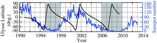
Figure 2. Heliographic latitude of Ulysses orbit (in black) and monthly sunspot number (in blue; http://sidc.oma.be/sunspot-data/). Gray shading indicates the two periods used in this paper: the minimum between cycles 22 and 23 (1995–1998) and the minimum between cycles 23 and 24 (2006–2010).
Download figure:
Standard image High-resolution imageOur focus in this study is on the PCH and ECH wind. To maximize our database we use an extended interval for the first minimum (1995–1998) to include as much ECH wind as possible measured by Ulysses since the equatorial ACE measurement was not available then. In the second minimum (2006–2010), we chose the start date as the time when the sunspot number was at the same level as at the start date of the first minimum, and the end date was chosen as the time when the sunspot number started to rise. The fact that the second minimum is longer than the first one is due to the fact that the second minimum is historically the most prolonged and weakest minimum in the modern space age (Cionco & Compagnucci 2012; Nandy et al. 2011; Zhao et al. 2013b; Fröhlich 2013). In situ observations of ECH and PCH winds from Ulysses and ACE during these two solar minima are then analyzed. During the first minimum before 1998, PCH and ECH winds were measured only by Ulysses, while during the second minimum the PCH wind was observed exclusively by Ulysses, and the ECH wind data is a combination of both Ulysses and ACE measurements.
3.1. Kinetic Properties
Histograms of the kinetic properties of the PCH and ECH wind, namely the proton speed; proton number density, which is normalized by the square of the heliocentric distance (R/ua, in Astronomical unit); and the proton flux are plotted in Figure 3. The top row shows the measurement of PCH wind, and the ECH wind is illustrated in the bottom row; the histograms of the first minimum are plotted as solid lines, while the second minimum is shown as dotted lines.

Figure 3. Histograms of PCH (ECH) solar wind proton speed (Vp), proton density (Np, normalized by heliocentric radius distance square (R/ua)2), and proton flux (Vp · Np, also normalized by (R/ua)2). Results obtained at the first minimum are shown by the solid lines and the second minimum by the dotted lines; PCH (ECH) is shown in the top (bottom) row.
Download figure:
Standard image High-resolution imageIn principle, the solar wind proton flux, as defined by the product of the proton number density (Np) and proton speed (Vp), is conserved in a flux tube along the heliocentric distance (R/ua). With the radial expansion of the flux tube, the cross section of the flux tube increases as (R/ua)2 so that the solar wind proton density decreases by a factor of (R/ua)−2; several studies confirmed that Np varies roughly along R/ua as a power law of (R/ua)−2 (Liu et al. 1995; Ebert et al. 2009). Therefore, in order to eliminate this flux-tube radial expanding effect and to compare the Np and the proton flux observed by Ulysses and ACE at different heliocentric distances, in Figure 3 the Np and proton flux are normalized by (R/ua)2.
The proton speed displayed in Figures 3(a) and (b) shows at least three interesting properties: (1) the PCH wind is faster than the ECH wind: most of the PCH wind is faster than 700 km s−1, while the majority of the ECH wind lies below 700 km s−1; (2) the proton speed decreased in the second minimum compared with the first minimum in both PCH and ECH winds; and (3) the shape of the distribution of the ECH wind significantly changes from the first minimum to the second minimum, with its peak shifting toward the low velocity side of the distribution and the 600 km s−1 cutoff; at the same time, the distribution of the PCH wind shifts by a small amount, without changing its shape. The average values, standard deviations, and changing rates of proton speeds in the two solar minima are given in Table 2.
Table 2. Averages and Changing Rates of PCH and ECH Wind Measurements from Ulysses and ACE at the Two Solar Minima
| Mean (Standard Deviationa) | PCH Wind | ECH Wind | ||||
|---|---|---|---|---|---|---|
| 1st Minimum | 2nd Minimum |  |
1st Minimum | 2nd Minimum |  |
|
| Vp(km s−1) | 784.9(14.0,13.4) | 761.5(16.2,14.6) | −2.98% | 673.7(13.9,19.7) | 642.1(20.5,12.0) | −4.69% |
| Np(cm−3) | 2.251(0.25,0.19) | 1.910(1.14,0.27) | −15.1% | 3.445 (1.81,0.67) | 3.070(1.17,0.44) | −10.9% |
| Vp · Np(cm−2 s−1 × 10⁸) | 1.77(0.19,0.15) | 1.46 (0.87,0.20) | −17.5% | 2.30(1.1,0.4) | 1.94(0.7,0.3) | −15.2% |
| Tp · (R/ua)0.54(MK) | 0.246(0.03,0.02) | 0.220(0.05,0.02) | −10.7% | 0.217(0.06,0.03) | 0.180(0.04,0.03) | −17.4% |
| Entropy | 12.00(0.09,0.10) | 11.98(0.2,0.10) | −0.2% | 11.70(0.13,0.12) | 11.52(0.19,0.15) | −1.6% |
| O7 +/O6 + | 0.0156(0.006,0.004) | 0.0113(0.008,0.003) | −38.1% | 0.0157(0.007,0.004) | 0.0155(0.005,0.003) | −1.91% |
| C6 +/C5 + | 0.139(0.03,0.02) | 0.077(0.04,0.02) | −44.6% | 0.160(0.05,0.04) | 0.166(0.05,0.04) | 3.75% |
| 〈Q〉Fe | 10.498(0.3,0.3) | 10.103(0.5,0.4) | −3.76% | 9.968(0.9,0.4) | 9.412(0.2,0.3) | −5.58% |
| Fe/O | 0.0593(0.01,0.01) | 0.0545(0.02,0.01) | −8.09% | 0.045(0.01,0.01) | 0.059(0.01,0.01) | 31.1% |
| He/p | 0.045(0.006,0.004) | 0.048(0.09,0.006) | 5.1% | 0.048(0.006,0.006) | 0.031(0.008,0.006) | −36.2% |
| |Br · (R/ua)2|(nT) | 2.93(0.86,0.84) | 2.35(0.91,0.67) | −19.8% | 4.71(3.3,1.3) | 2.59(1.04,0.74) | −45.0% |
Note. aThe first (second) value is the standard deviation of the distribution above (below) the mean value.
Download table as: ASCIITypeset image
The proton number density is shown in Figures 3(c) and (d). Comparing these two figures, we find that the distribution of the proton number density of PCH wind is much narrower than for ECH wind in both minima. Also, the proton number density of ECH wind is larger than PCH wind on average. Both types of wind experience a slight reduction of the average proton number density in the second solar minimum compared with the first minimum. However, while PCH keeps the shape of its distribution almost unchanged, the distribution of ECH wind is slightly narrower. The average values, the standard deviations, and the rates of change are listed in Table 2.
Both the differences in PCH and ECH wind proton speed and density contribute to the difference in proton flux, as shown in Figures 3(e) and (f). In fact, the proton flux in PCH wind is distributed in a narrower range than in the ECH wind at both solar minima. Also, the proton flux in the second minimum decreases at similar rates in both of the winds, and its distribution is unaltered in PCH but narrows in ECH, compared with the first minimum. In general, the values of proton flux in these two kinds of coronal hole winds look rather similar, while their averaged values, as listed in Table 2, indicate that the average proton flux in ECH wind is slightly larger than in the PCH at both minima.
3.2. Thermal Properties
Helios observations (Marsch et al. 1982; Schwenn et al. 1981) and Ulysses observations (Liu et al. 1995; Ebert et al. 2009) showed that the proton kinetic temperature in fast and slow wind decreases with distance following a power law of (R/ua)−α, because of adiabatic cooling. The adiabatic cooling's effects are stronger in slow solar wind than in the fast wind (Liu et al. 1995). In the fast solar wind, due to different interaction processes, the solar wind plasma can also be heated by multiple interplanetary sources, i.e., turbulence dissipation or shocks (Tu 1988; Whang 1991), so that its proton temperature profile is flatter (α is smaller) than in the slow wind. Especially, the larger the heliocentric distance from about 0.3 ua to ≈5 ua, the more heating the fast wind plasma receives from wave damping or turbulence dissipation, resulting in a smaller value of α and a flatter curve of temperature profile (Cranmer 2009). In this work, rather than assuming unity α and scaling the proton temperature by R/ua (Ebert et al. 2013; Elliott et al. 2012), we fit the fast wind (defined as Vp > 600 km s−1) as measured from Ulysses by a power law of (R/ua)−α, finding that α is about 0.54 (Figure 4).
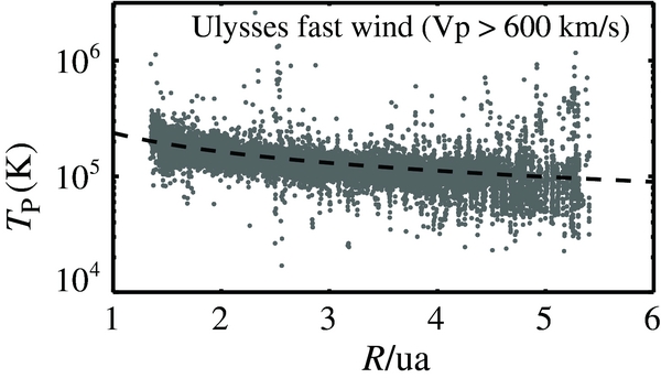
Figure 4. Proton temperature of the fast solar wind (Vp > 600 km s−1, gray dots) versus the heliocentric distance (R/ua), measured by Ulysses from 1991 January 1 to 2009 June 30. ICMEs are excluded. The dashed line is the power law fitting, Tp = 237,749(R/ua)−0.543 K.
Download figure:
Standard image High-resolution imageIn Figure 4, the proton temperature of the bulk of the fast solar wind is plotted versus the heliocentric distance, R, where ICMEs are excluded using Ulysses ICME list given by Ebert et al. (2009). The power law of R−α fitted curve is illustrated by the dashed line, which is Tp = 237 749(R/ua)−0.543. Therefore, in this study, we normalize the observed proton temperature by a factor of (R/ua)0.543 in order to compare the proton temperature measured by Ulysses with the ACE measurement at 1 ua.
Figures 5(a) and (b) present the comparison of the normalized proton temperature as measured by Ulysses and ACE at the two minima, for the PCH wind and ECH wind, respectively. As shown in Figures 5(a) and (b), the proton temperature in these two types of CH wind looks different in at least two ways. First, the shapes of the distributions of proton temperature in these two types of wind are different: PCH has narrower distributions than ECH wind. This difference is present in both solar minima. Second, during each solar minimum, on average, PCH wind has higher proton temperature than ECH wind. This trend is consistent with the fact that PCH wind is generally faster than ECH wind and proton temperature is proportional to solar wind proton speed for the first order of approximation (Elliott et al. 2012).

Figure 5. Histograms of the proton temperature Tp and proton-specific entropy, ln[(Tp/K)/(Np/cm−3)0.5], of PCH wind (top row) and ECH wind (bottom row) at the first minimum (solid lines) and the second minimum (dotted lines), where Tp is normalized by (R/ua)0.543 and Np is normalized by (R/ua)2.
Download figure:
Standard image High-resolution imageThe comparison between the two minima in each type of wind shows that at the second minimum the proton temperature in both PCH and ECH wind decreased compared with the first minimum, but the shapes of their distribution remain nearly the same. The averaged values, the standard deviations, and the rates of change are listed in Table 2.
The proton-specific entropy (called entropy hereafter), as a measure of the disorder of an isolated thermal system, always increases in a thermodynamic process and reaches its maximum at the equilibrium state. In the solar wind plasma, this quantity is proportional to ln[(Tp/K)/(Np/cm−3)(γ − 1)], where Tp is the proton kinetic temperature and Np is the proton density. In this study, we assume γ = 1.5 (Siscoe & Intriligator 1993; Burton et al. 1999) and scale the Tp and the Np measured by Ulysses by factors of (R/ua)0.543 and (R/ua)2, respectively, as discussed above. On the basis of the ACE measurements during solar cycle 23, it has been found that the entropy is highly anticorrelated with the O7 +/O6 + ratio in the rising phase (1998–1999) for the nontransient solar wind. This correlation is weakened during the solar maximum where ICMEs and shocks are much more frequent (Pagel et al. 2004). Therefore, entropy has been considered to be a good proxy for the O7 +/O6 + ratio in studies of the quiet solar wind plasma during the Sun's low activity phase. Recently, by using entropy to examine the fast and slow interface, Crooker & McPherron (2012) found that entropy shows a very sharp transition at the fast/slow wind interface: it suddenly increases from the slow wind side to the fast wind side at the transition.
Figures 5(c) and (d) show the distributions of entropy of the PCH and ECH wind in the two minima, respectively. There are several points worth noticing. First, the entropy of PCH is higher than ECH at both of the solar minima; this is consistent with the fact that the PCH wind is faster than ECH wind (Figures 3(a) and (b)). Second, from the first to the second minimum, the entropy decreased in both winds, but by different amounts, with the decrease in the ECH wind being much larger than in the PCH wind. Third, the shape of the distribution of the entropy in PCH wind is slightly narrower than in ECH wind at each of the solar minimum, which might be a direct consequence of the narrower shapes of the proton density and temperature of PCH wind (Figures 3(a) and 5(a)). The average values, standard deviations, and rates of change of the entropy in the two types of coronal hole winds at the two minima are listed in Table 2.
3.3. Compositional Properties
Some key compositional properties of the PCH and ECH winds, namely the charge state ratios and the elemental abundance ratios, are shown in Figures 6 and 7 with the same conventions as in Figure 3.
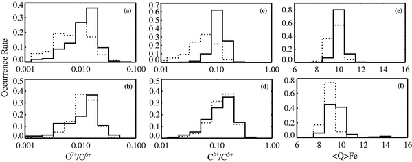
Figure 6. Histograms of the ionic charge state ratios O7 +/O6 + and C6 +/C5 + and the average charge state of Fe (〈Q〉Fe), PCH wind (top row), and ECH wind (bottom row) at the first minimum (solid lines) and the second minimum (dotted lines).
Download figure:
Standard image High-resolution image
Figure 7. Histograms of elemental abundance ratios of iron to oxygen (Fe/O) and helium to proton (He/p) of PCH wind (top row) and ECH wind (bottom row) at the first solar minimum (solid line) and the second minimum (dotted lines).
Download figure:
Standard image High-resolution imageFigure 6 displays the ionic charge state signatures, namely the O7 +/O6 + and C6 +/C5 + ratios and the average charge state of iron (〈Q〉Fe), of these two types of coronal hole winds at the two minima. By examining each row, we can compare the difference between the two minima for each type of the wind separately. For PCH wind (top row), we find that all charge state signatures decreased in the second minimum compared with the first minimum (Figures 6(a), (c), and (e), also see Table 2). This result is consistent with von Steiger & Zurbuchen (2011), which shows the evolution of the polar solar wind (also defined as |λ| > 70° but without any constraints on speed or charge state ratio as we do in this paper) observed by Ulysses in its first and third high latitudinal scans around the solar minimum conditions in 1994–1995 and in 2007–2008.
Table 2 lists the average values, the standard deviations, and the changing rates of the results in this comparison. The decreasing rates of the O7 +/O6 + and C6 +/C5 + ratios in PCH winds are −38.1% and −44.6%, respectively, while the fractional decrease in 〈Q〉Fe is 3.76% in PCH wind. Although the decreasing rate of the average value of 〈Q〉Fe is only a few percent, such change implies a large variation of the abundance of each individual Fe ion, as shown in Figure 6(e). For example, the increase of the fraction of Fe9 + at the second minimum in PCH wind is huge, and so is the decrease of Fe10 + and Fe11 + (Figure 6(e)). In addition, the shape of the O7 +/O6 + and C6 +/C5 + ratios in PCH changes significantly between the two cycles, becoming broader in the second minimum.
The bottom row of Figure 6 shows the charge state composition of ECH wind. Unlike the PCH wind, the solar cycle variation of the ionic charge state ratios, O7 +/O6 + and C6 +/C5 +, of the ECH wind are moderate. However, the decrease in 〈Q〉Fe of the ECH wind is even more dramatic than in the PCH wind, indicating a much different evolution of this element between these two minima in ECH wind. For example, the increase in the fraction of Fe9 + and the decrease in Fe10 + are so significant that they make the whole distribution of 〈Q〉Fe in ECH wind at the second minimum shifted to the left side and turned narrower than the first minimum (Figure 6(f)). Therefore, we find that the charge state distribution of the PCH and ECH winds responds very differently to the strength of the solar cycle.
Figure 6 also shows the differences between PCH and ECH winds when considered within the same minimum; the values of the O7 +/O6 + and C6 +/C5 + ratios in the ECH are larger than in the PCH wind at each solar minimum, while the 〈Q〉Fe of ECH wind is always significantly lower than PCH wind at all times.
The comparison of the elemental abundance ratios, the iron to oxygen total density ratio (n(Fe)/n(O), Fe/O hereafter) and the helium to proton total density ratio (n(He)/n(p), He/p hereafter), in both PCH and ECH winds at the two minima is shown in Figure 7, where the top row shows the measurement of the PCH wind, the bottom row represents the ECH wind, the solid histograms indicate the distributions at the first minimum, and the dotted lines illustrate the second minimum. Comparing the solid and dotted histograms at the top and bottom rows, we find that the evolution of the element abundance ratios of the two types of wind is very different. The Fe/O and He/p ratios of the PCH stay almost the same at the two minima (the top row, Figures 7(a) and (c)), while in the ECH wind, the fractional increase in the average value of Fe/O is 31.1% (shown by the apparent right-sided shift of the dotted histogram in Figure 7(b)) and the fractional decrease in the average of He/p is 36.2% (illustrated by the obvious left-sided shift of the dotted histogram in Figure 7(d)) at the second minimum compared with the first minimum. Second, the shape of the Fe/O distribution in the ECH wind approaches the one of the PCH wind at the first and the second minimum, while that of the He/p ratio in ECH wind becomes wider than PCH wind at the first and the second minimum. The dramatic decrease of the He/p ratio in the ECH wind at the second minimum compared with the first minimum is also reported by Kasper et al. (2012) and McIntosh et al. (2011), based on their analysis of WIND data. They confirm that the decrease in solar wind helium abundance during the cycle 23–24 minimum compared with the previous minimum is a phenomenon that is much more apparent in the equatorial relatively fast speed wind than in slow speed wind. We will give more discussion about these variations of the elemental abundance in the discussion section.
3.4. Radial Open Magnetic Flux
Coronal holes, as the regions where the Sun's open magnetic field lines primarily come from, are always dominated by strong open magnetic flux (as defined by the radial component of the magnetic field, Br, normalized by heliocentric distance square, (R/ua)2; we call it as Br flux hereafter). Since the second solar minimum, the strength of the heliospheric magnetic field has been reported to rapidly decrease to a level never observed during the space age; the fractional decrease of the Br flux is 30% from the value of the previous minimum (e.g., Smith & Balogh 2008; Zhao & Fisk 2011). The question is, how much did the variations of Br flux in PCH and ECH regions contribute to this dramatic reduction?
In Figures 8(a) and (b), the absolute value of Br flux of PCH and ECH wind at the two minima is shown in the top and bottom figures, respectively. In both winds, Br flux significantly decreased during the second minimum compared with the first one, as shown by the shifts of the dotted histograms to the left side. The largest change is experienced by the ECH wind both in the distribution shape and in the average Br flux value. The fractional decreases in the average values of Br flux are 19.8% and 45.0% in the PCH and ECH wind (Table 2), respectively. In addition, on average, the Br flux in ECH is always larger than it is in PCH for both minima, with a significant difference between them at the first minimum but somehow a slight difference at the second minimum after the substantially decrease of Br flux in the ECH wind. In addition, the distribution of Br flux in ECH wind is much narrower during the second minimum than it is at the first minimum.
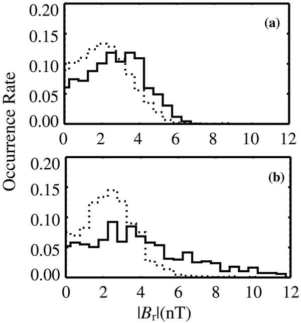
Figure 8. Histograms of absolute values of Br flux (Br normalized by (R/ua)2) in PCH wind (top) and ECH wind (bottom) at the first minimum (in solid lines) and the second minimum (in dotted lines).
Download figure:
Standard image High-resolution image3.5. Summary of the Comparative Study
The main results of the comparison between the ECH and PCH winds are that (1) they are two very different types of fast wind, and (2) they evolve in different ways during the solar cycles. In particular:
- 1.ECH protons are generally slower than PCH protons at the two minima. PCH wind and ECH wind can be well separated by a threshold of 700 km s−1. The average fractional reduction of the proton speed in PCH and ECH wind during the second minimum is less than 5%, but the distribution shape of the ECH proton speed changes significantly.
- 2.The proton number density and flux are higher and distributed in a wider range in ECH wind than in PCH wind during both minima. The rates of decrease of the proton density and flux from the first minimum to the second minimum are close in these two types of winds.
- 3.The proton temperature is higher and distributed in a narrower range in PCH wind than in ECH wind at each solar minimum. During the second minimum, it decreases in both winds compared with the first minimum.
- 4.The entropy of the PCH wind is larger and more narrowly distributed than the entropy of the ECH wind at each minimum. The decrease of entropy during the second minimum compared with the first minimum in ECH wind is larger than in PCH wind.
- 5.The O7 +/O6 + and C6 +/C5 + ratios dramatically decrease in PCH wind at the second minimum compared with the first; however, their variations in the ECH wind are far smaller. Also, these ratios are larger in ECH wind than in PCH wind during both minima. Average values of 〈Q〉Fe at the second minimum in both winds decreased by small rates; however, this small variation results in large changes in the relative abundance of some Fe ions, such as Fe9 + and Fe10 +. Also, unlike O7 +/O6 + and C6 +/C5 +, 〈Q〉Fe is higher in PCH wind than in ECH for both of the solar minima.
- 6.The Fe/O and He/p ratios are almost constant in PCH wind at the two minima, whereas in ECH wind, Fe/O increases and He/p decreases dramatically during the second minimum compared with the first minimum.
- 7.The Br flux decreases in both PCH and ECH wind during the second minimum, with the reduction rate in ECH wind (≈45%) being much larger than in PCH wind (≈20%).
4. REMOTE SENSING OBSERVATIONS
The differences between the ECH and PCH winds can be crudely summarized by saying that the former type of wind is slower and denser than the latter, its O7 +/O6 + and C6 +/C5 + charge state ratios are higher, but its 〈Q〉Fe is significantly lower. Also, the two winds evolve differently with the solar cycle. These results beg the question of whether such strikingly different characteristics are due to differences in the structure and wind history in the source regions or to some mechanism that differentiates those two types of winds at high altitude from plasmas with similar properties closer to the Sun. This brings our attention to the properties of the PCH and ECH winds close to the Sun, within the field of view of space-borne EUV imaging and spectroscopic instruments.
It is important to note that ECHs are best studied when observed on the disk, since at the limb their emission is heavily contaminated by the brighter emission from streamer plasma along the line of sight. The coronal temperature of ECHs was measured by Chiuderi Drago et al. (1999) using radio observations and was found to be similar to the temperature of PCH regions; a similar result has been found by Del Zanna & Bromage (1999) using SOHO/CDS. However, no direct comparison has been made with polar holes. Both those measurements belong to cycle 23: to the best of our knowledge no such comparison has been done during the minimum between cycles 23 and 24 (the second minimum) by using instruments either on board SOHO or Hinode. Higher in the solar corona, Miralles et al. (2001b) used SOHO/UVCS to determine the electron density and plasma velocity of the ECH wind between 1.5 and 3.0 solar radii ( ) and found that the plasma was denser and much slower than its PCH counterpart, indicating that the differences that we found between ECH and PCH are already present in the inner corona.
In order to investigate whether PCH and ECH harbor any difference in the corona, and whether and to what extent these differences are propagated from cycle 23 (the first minimum) to cycle 24 (the second minimum), we have determined the plasma thermal distribution of ECHs and PCHs in these two minima. A thorough, systematic study of the evolution of these two structures along the solar cycle is beyond the scope of the present paper and is deferred to a future work; here we limited our analysis to an ECH/PCH pair for each cycle. Observations for the first minimum were taken by SOHO/CDS and those for the second minimum were taken by Hinode/EIS. The details of the observations are reported in Table 3.
Table 3. Parameters of the Coronal Hole Observations on the Disk
| First Minimum | Second Minimum | |||
|---|---|---|---|---|
| ECH | PCH | ECH | PCH | |
| Date | 1996 Aug 27 | 1996 Jul 1 | 2007 Mar 31 | 2009 Apr 23–25 |
| Pointing | (109'', 72'') | (118'', 844'') | (179'', –143'') | (0'', −1050'') |
| Field of view | 41'' × 240'' | 20'' × 240'' | 210'' × 512'' | 90'' × 512'' |
| Log[Ne/(cm−3)] | 8.10 | 7.65 | 8.20 | 8.10 |
| He | I | I | II | II |
| C | III | III | ||
| N | IV–V | IV | ||
| O | II–V | II–V | IV–V | IV–V |
| Ne | IV–VII | IV–VII | III | |
| Mg | IV–X | IV–X | V–VII | V–VII |
| Si | VIII–X | VIII–X | VII–VIII, X | VI–VII, IX–X |
| S | X | X, XI | ||
| Ca | VIII, X | VII–VIII, X | ||
| Fe | X–XII | X–XII | VIII–XV | VIII–XV |
Notes. Stages of ionization are indicated as follows: He i stands for He0 +, O ii for O1 +, O iii for O2 +, and so on.
Download table as: ASCIITypeset image
The sample of observations used in the present work is far from being exhaustive: we only selected a few examples to show the major features of the thermal structures of ECH and PCH regions in two different solar cycles. A more comprehensive and systematic study of the characteristics and evolution along the solar cycle of these two regions is deferred to a future work. For each region we have selected data sets that included the full spectral range of the instruments, in order to maximize the number of ions that provided lines suitable for analysis. Each of the data sets has been reduced, cleaned, and calibrated using the standard software made available by the instruments' teams in SolarSoft. We have selected the areas of the field of view corresponding to on disk portions of the coronal hole, since we were interested in determining the thermal structure for the entire line of sight, including chromosphere and transition region. Also, we selected ECH data sets observed near disk center, where contamination from nearby streamer plasma was minimal; PCH data sets are close to the limb and belong to large PCH regions. By assuming that the plasma is optically thin, we restricted our analysis to plasmas hotter than 100,000 K, as below those temperatures optical thickness can affect both emerging line radiances and ion level populations.
Since the solar wind plasma charge state composition is affected by the electron density and temperature, we determined the distribution of plasma with temperature, which is usually described by the plasma differential emission measure (DEM) φ(T), defined as

The DEM has been determined using the iterative diagnostic technique of Landi & Landini (1997). This technique allows to determine the DEM of the plasma from observed line radiances starting from an initial, arbitrary DEM φ0(T), and the correction is determined by calculating a correction function ω0(T) to the curve φ0(T) using line radiances. Comparing the observed line radiances with the values predicted using φ0(T) as
where G(T, Ne) is the line Contribution Function, which includes the atomic physics constants and transition rates involved in the process of line emission. This function depends on both the electron temperature and density. Each line i provides a correction to φ0(T) at an effective temperature
The corrections  provided by all lines are interpolated as a function of T to produce the correction function ω0(T), which is used to calculate an improved DEM curve as

Observed line radiances are then used to calculate a new correction curve ω1(T) to φ1(T). The procedure is repeated until the nth correction function ωn(T) is unity within uncertainties. Convergence is usually very fast. The Contribution Functions were calculated as a function of electron temperature using values of the electron density measured using line radiance ratios. We used the radiance ratios between the Fe xiii 203.8 Å and 202.0 Å lines (EIS; data sets at first minimum) and the Si ix 341.9 Å and 345.0 Å lines (CDS; data sets at second minimum) to determine the electron density values of each data set, reported in Table 3. It is interesting to note that in both cycles the ECH electron density is larger than the PCH value. The Contribution Functions were calculated using version 7.1 of the CHIANTI database (Landi et al. 2013), adopting the combination of the photospheric abundances of Caffau et al. (2011) and Lodders et al. (2009) provided by CHIANTI, as well as the CHIANTI ionization equilibrium calculations.
The resulting DEM curves are shown in Figure 9 for the PCH and ECH data sets observed during the first minimum and in Figure 10 for those observed during the second minimum. Individual DEM determinations provided by each line are also shown. All DEM curves show a few common features: the amount of plasma in the lower transition region (log T/K ≈ 5.0 to 5.3) decreases very rapidly; a first DEM maximum occurs at temperatures log T/K ≈ 5.5 to 5.7, and a second maximum, corresponding to the corona, occurs at log T/K ≈ 5.9 to 6.1; and at larger temperatures, the amount of material decreases very quickly. These DEM shapes are typical of coronal holes (e.g., Phillips et al. 2008, and references therein). No need was found to change the relative abundances of the elements, so that the element composition of both regions in both cycles was approximately the same.

Figure 9. CDEM curve for ECH and PCH during the first minimum. Red: ECH; Blue: PCH. DEM determinations provided by each individual spectral line are indicated with error bars.
Download figure:
Standard image High-resolution image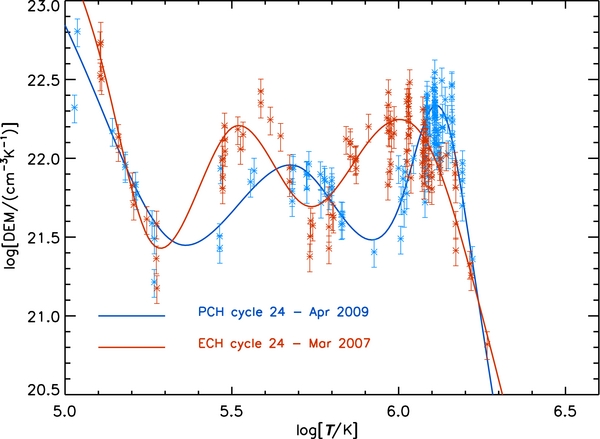
Figure 10. DEM curve for ECH and PCH during the second minimum. Red: ECH; Blue: PCH. DEM determinations provided by each individual spectral line are indicated with error bars.
Download figure:
Standard image High-resolution imageThe DEMs of the first minimum have very similar shape, although the coronal peak is much larger in the ECH region than in PCH, indicating that much more material is available in the ECH corona than in the PCH one; still, the temperature of the peak is essentially the same in both PCH and ECH. Also, the DEM peak maximum in the transition region is much smaller than the one in the corona. In the second minimum the ECH and PCH DEM curves show larger differences. In fact, while still showing the double peak structures, the peak values are approximately the same in both curves; also, the temperature of both peaks are larger in the PCH than in the ECH.
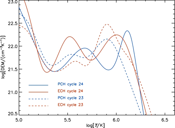
A comparison of the DEM curves of both minima is shown in Figure 11 and indicates that the DEM of both ECH and PCH from different cycles show large variations. The coronal portion of the DEM is hotter in the second minimum than it was in the first minimum; the transition region portion has increased its size, and in the case of the PCH, it is also hotter. Figures 9, 10, and 11 show that (1) the thermal distribution of the plasma in the ECH and PCH is indeed different, (2) it changes between two different cycles, and (3) PCH and ECH evolve differently in different cycles. Also, the ECH plasma is denser than the PCH one.
Figure 11. Comparison of DEM curves at the two minima. Red: ECH curves; Blue: PCH curves.
Download figure:
Standard image High-resolution image
5. DISCUSSION
The results from the in situ measurements indicate that the ECH wind plasma in the Heliosphere is slower and denser than the PCH wind and has significantly different charge state and element composition from the latter. These differences can be attributed to three possible causes: (1) the mechanism accelerating the ECH and PCH wind on the solar corona could be different, or (2) the acceleration mechanism is the same, but the ECH wind is accelerated from a source region with different properties than the PCH wind (namely, ECH has different properties from PCH), or (3) the interaction with the equatorial slow wind streams can affect the ECH wind properties significantly during its propagation in the heliosphere, while such interaction is not experienced by the PCH wind.
Interchange reconnection is one of the most promising candidate mechanisms of solar wind acceleration for all of the nontransient solar wind (ICMEs excluded). According to this scenario, after one foot of a magnetic loop reconnects with an opposite-polarity open magnetic flux, the loop opens up and releases its plasma into the solar wind (Fisk 2003). The direct consequence of this process is the mass flux, and the final speed of the solar wind is completely determined by the properties of the reconnecting magnetic loop. Specifically, the solar wind final speed is anticorrelated to the loop electron temperature, regardless of where the solar wind is accelerated from (in streamer or in coronal holes), and of the solar wind type (fast wind or slow wind). This anticorrelation has been confirmed by Ulysses measurements of fast and slow wind (Gloeckler et al. 2003) and by ACE measurements during the past two solar minima (Zhao & Fisk 2011; Zhao et al. 2013a). In all of these previous studies, there are no distinct subgroups in the fast speed range (>600 km s−1); instead, the fast wind shows a continuum of anticorrelating distribution in the speed-versus-electron-temperature plot (i.e., Zhao & Fisk 2011). Therefore, the validation of this anticorrelation between the solar wind final speed and their coronal electron temperature in the PCH and ECH wind demonstrates that these two types of fast wind are accelerated by the same interchange reconnection process. Thus, the first hypothesis can be ruled out.
To test the scenario that the ECH wind properties are affected by the equatorial slow wind, we examine the influence of the Streamer Interaction Regions (SIRs) including the Corotating Interaction Regions (CIRs) on our results. We find that by removing the SIR and CIR intervals (Jian et al. 2006) from our ACE database, the results do not show any noticeable changes from before. Also, the Fe/O ratio is very similar in both PCH and ECH wind, while the slow wind value is much larger (Zhao & Landi 2013). In case the ECH and slow wind plasma interacted, we would expect the ECH Fe/O ratio to be larger than the PCH ratio, contrary to the results shown in Figure 7. As a consequence, the significant differences in the PCH and ECH wind are not caused by the impact of SIRs or CIRs on the ECH wind, but they are indeed attributed to the different properties of the PCH and ECH regions at the corona source. Thus, the third hypothesis can be ruled out.
Significant differences in the outflow velocity and density between PCH and ECH wind had already been found by Miralles et al. (2001b, 2002, 2006). They analyzed the observations from the UVCS aboard SOHO and found that the O5 + outflows from the ECH regions (at solar maximum of cycle 23) were characterized by a lower speed of only ≈100 km s−1 and higher density at 3 RSun than the outflows originated from PCH regions at the solar minimum between solar cycles 22 and 23, where their speed could reach ≈400 km s−1 at the same distance of 3 RSun.
The low-latitude section of the Elephant Trunk coronal hole observed in the previous minimum (1996) also showed a slower speed than the typical fast solar wind from the poles (Bromage et al. 2000). This slight yet noticeable difference in the solar wind speed between the PCH and ECH winds could be related to the difference in the size and width of these two types of coronal holes (i.e., Zhang et al. 2003). In fact, ECHs like the "elephant trunk" have smaller size and narrower width than a classic PCH, which can occupy large area at solar pole during solar minimum. Numerical models show that smaller and narrower ECHs have larger magnetic expansion factors than the larger and wider PCHs (Wang et al. 1996). Therefore, the reduction in solar wind speed in the ECHs is consistent with the empirical anticorrelation found between the solar wind speed and the magnetic expansion factor in their coronal source region (e.g., Wang & Sheeley 1990; Arge & Pizzo 2000).
The compositional difference in the PCH and ECH winds can also be explained by the different properties of PCH and ECH regions in the solar corona. Spectroscopic studies revealed that the PCH and ECH winds have a different speed already very close (≈3 RSun) to the Sun (i.e., Miralles et al. 2001b). This means that the ECH wind plasma spends more time at every location along its trajectory than the PCH wind. In addition, since ECH plasma density is larger than in PCHs, the ECH wind plasma ionization is expected to be more sensitive to the local electron temperature than PCH wind. In fact, in the inner corona, the electron temperature of coronal holes increases with distance from the photosphere until it reaches a maximum, and then it decreases (Geiss et al. 1995; von Steiger & Zurbuchen 2011). For carbon and oxygen, their freeze-in height is below the temperature maximum. In the ECH wind where the solar wind plasma is slower and denser, carbon and oxygen freeze-in at a larger distance and at a higher charge state ratio than in the PCH wind where the plasma is less sensitive to the increasing electron temperature.
The lower 〈Q〉Fe values in the ECH can also be explained by the same scenario, considering the Fe freezes-in at much larger distances, beyond the temperature maximum. In this case, the denser ECH wind is more sensitive to the decrease in temperature, resulting in an overall lower average ionization. Similar qualitative statements can be applied to the results of both cycles.
However, in the second minimum, all charge state proxies decreased (except that C6 +/C5 + in ECH wind has a slightly increase), indicating a lower degree of ionization of the plasma, even if both plasmas decreased their velocity, and remote sensing measurements indicate hotter and denser source region plasmas. The dramatic decrease of the O7 +/O6 + and C6 +/C5 + ratios in PCH wind may be due to the larger amount of material at transition region temperatures, which could bias their values toward lower ionization; the lower density of the corona relative to the transition region prevents the former to ionize C and O enough to reach cycle 23 values (Figure 11). The large decrease in the average Fe ionization 〈Q〉Fe of both winds can also be explained, even in the presence of a hotter and denser inner corona, by the decrease in wind velocity, which lets both winds spend more time beyond the temperature maximum of the corona so that they can experience reduced ionization and increased recombination.
Understanding whether, and to what extent, the differences in the thermodynamic properties of the coronal regions where the ECH and PCH wind originate are responsible for the differences in the wind properties measured in situ requires a detailed forward modeling work, which is able to predict the charge state composition of the wind starting from the thermal properties of its source region. Such a forward modeling requires the solution of the system of equations that governs the wind plasma ionization and recombination as the wind travels from its source region in the chromosphere through the transition region and the corona, as well as the coupling of the results to the CHIANTI spectral code to predict the wind EUV line emission to be compared with remote sensing observations. Such a forward modeling has been recently discussed by Landi et al. (2012) and references therein. However, quantitative analysis requires that the in situ plasma and the EUV observations involve the same stream of plasma, while in the present work we only selected a few regions in the solar corona that do not correspond to the in situ data we analyzed. Thus, we defer such a detailed forward modeling to a future paper, and we only present a qualitative discussion here.
6. SUMMARY
In this work, we compare the PCH and ECH winds based on their in situ and spectroscopic observations and find that PCH and ECH regions have different thermal properties that can be the driver for the in situ differences we found between these two types of wind. Further, both regions and their winds changed from the first solar minimum (between cycles 22 and 23) to the second minimum (between cycles 23 and 24), and their evolution is also different. These results suggest that ECH and PCH are indeed two separate types of regions rather than being the same type of region that happens to be observed at different latitudes; also, the winds they produce make two separate subcategories of fast wind.
The work of L.Z. and E.L. was supported by NASA grant NNX11AC20G.