


ABSTRACT
Supermassive black hole (SMBH) binaries are expected in a ΛCDM cosmology given that most (if not all) massive galaxies contain a massive black hole (BH) at their center. So far, however, direct evidence for such binaries has been elusive. We use cross-correlation to search for temporal velocity shifts in the Mg ii broad emission lines of 0.36 < z < 2 quasars with multiple observations in the Sloan Digital Sky Survey. For ∼109 M☉ BHs in SMBH binaries, we are sensitive to velocity drifts for binary separations of ∼0.1 pc with orbital periods of ∼100 yr. We find seven candidate sub-parsec-scale binaries with velocity shifts >3.4σ ∼ 280 km s−1, where σ is our systematic error. Comparing the detectability of SMBH binaries with the number of candidates (N ⩽ 7), we can rule out that most 109 M☉ BHs exist in ∼0.03–0.2 pc scale binaries, in a scenario where binaries stall at sub-parsec scales for a Hubble time. We further constrain that ⩽16% (one-third) of quasars host SMBH binaries after considering gas-assisted sub-parsec evolution of SMBH binaries, although this result is very sensitive to the assumed size of the broad line region. We estimate the detectability of SMBH binaries with ongoing or next-generation surveys (e.g., Baryon Oscillation Spectroscopic Survey, Subaru Prime Focus Spectrograph), taking into account the evolution of the sub-parsec binary in circumbinary gas disks. These future observations will provide longer time baselines for searches similar to ours and may in turn constrain the evolutionary scenarios of SMBH binaries.
Export citation and abstract BibTeX RIS
1. INTRODUCTION
Supermassive black holes (SMBHs) were first proposed to account for the energy source of active galactic nuclei (AGNs; e.g., Robinson et al. 1965). Now it is well known that nearly every galaxy hosts an SMBH in its center (Kormendy & Richstone 1995). At the same time, in a ΛCDM cosmology, galaxies grow by hierarchical merging (White & Rees 1978), and galaxy mergers are directly observed (e.g., Schweizer & Seitzer 1992). During the merger, the SMBHs from each progenitor will sink to the center of the merger remnant, and therefore it seems inevitable that the two SMBHs will form a gravitationally bound pair, known as an SMBH binary (Begelman et al. 1980). Merging SMBHs are expected to be the strongest source of gravitational wave (GW) radiation for future space-based laser interferometers (Amaro-Seoane et al. 2013). However, the exact temporal evolution of these binaries, which directly determines their detection rates, remains uncertain from both a theoretical and observational perspective. Our goal in this paper is to place observational constraints on the highly uncertain sub-parsec phase of SMBH binary evolution.
SMBH binary systems evolve via the extraction of energy and angular momentum by the stars or gas in the vicinity, which makes the two black holes (BHs) spiral in and coalesce. A possible scenario for SMBH binary evolution in the relaxed stellar nucleus of two merging galaxies was first proposed by Begelman et al. (1980).
- 1.The two galaxies spiral into the galaxy center via dynamical friction. The BHs in the nuclei become gravitationally bound when the semi-major axis of their orbit reaches rB ∼ 32.2 pc (Mp/108 M☉)1/3(Nm*/3 × 109 M☉)−1/3(rc/100 pc) (Mp: primary (more massive) BH mass; N: number of stars in the central stellar core; m*: average stellar mass; rc: radius of the stellar core).
- 2.The binary orbit is hardened by restricted three-body interactions with stars during which the stars are ejected at velocities that are comparable to the orbital velocity of the binary. The binary becomes "hard" when its orbital velocity exceeds the velocity dispersion σ of the ambient stars, literally at rh ∼ 2.7 pc (1 + q)−1(Ms/108 M☉)(σ/200 km s−1) (Ms: secondary (less massive) BH mass; q: mass ratio Ms/Mp; Merritt & Milosavljević 2005). The typical hardening radius is ∼1 pc for BH binaries with comparable masses of ∼108 M☉ in each, in a stellar core with a typical velocity dispersion of 200 km s−1.
- 3.GW radiation becomes dominant in extracting angular momentum from the binary when the semi-major axis of the binary is less than rGR ∼ 0.016 pc q1/4(Mp/108 M☉)(th/108 yr)1/4 (th is the hardening timescale in step 2). For BH binaries with masses MBH ≈ 108 M☉ and fiducial values for the hardening timescale th ∼ 107–108 yr, this critical radius is around 10−3 to 10−2 pc.
It is still uncertain whether the transition from (2) to (3) can occur in less than a Hubble time. The SMBH binary will run out of stars to eject at a separation of ∼1 pc in an axisymmetric stellar potential (Quinlan 1996), so the extraction of angular momentum via star ejection is no longer efficient for separations of the binary BHs on sub-parsec scales. This is the so-called final parsec problem (Begelman et al. 1980; Milosavljevic & Merritt 2003). Many mechanisms have been proposed to overcome the final parsec problem, including gas accretion onto the binary (Armitage & Natarajan 2005; Gould & Rix 2000; Escala et al. 2004; MacFadyen & Milosavljević 2008; Cuadra et al. 2009; Rafikov 2013), refilling the loss cone by star–star encounters (Yu et al. 2005; Merritt & Wang 2005) and/or distorted stellar orbits in triaxial nuclei (Merritt & Poon 2004; Merritt & Vasiliev 2011). While it remains uncertain whether these mechanisms lead to a final coalescence within a Hubble time, it is certain that the binary will spend the longest time at sub-parsec separations (Begelman et al. 1980). In principle, sub-parsec SMBH binary systems may be very common. Unfortunately, in practice it has proven difficult to obtain definitive observational evidence of their existence.
1.1. Previous Searches for SMBH Binaries
There is indirect evidence for the presence of SMBH pairs at ∼kpc scales in single galaxies detected via both direct imaging (Junkkarinen et al. 2001; Komossa et al. 2003; Ballo et al. 2004; Comerford et al. 2009b; Fabbiano et al. 2011) and double-peaked narrow emission lines (Comerford et al. 2009a; Wang et al. 2009; Smith et al. 2010; Liu et al. 2010a, 2010b; Shen et al. 2011a). A parsec-scale BH pair CSO 0402+379 was detected with the Very Long Baseline Array (Maness et al. 2004; Rodriguez et al. 2006), and OJ 287 is believed to be a sub-parsec scale SMBH binary due to its periodic luminosity variations with a period of ∼11.86 yr (Takalo 1994; Pursimo et al. 2000; Valtonen et al. 2008). Indirect evidence for sub-parsec-scale pairs includes the precession of radio jets (Begelman et al. 1980; Liu & Chen 2007), double–double radio galaxies (Schoenmakers et al. 2000; Liu et al. 2003), the X-shaped radio sources (Dennett-Thorpe et al. 2002; Merritt & Ekers 2002; Liu 2004), and "light deficits" in the cores of elliptical galaxies (Milosavljević et al. 2002; Ravindranath et al. 2002; Graham 2004; Merritt 2006; Kormendy & Bender 2009).
However, there are no confirmed detections of sub-parsec SMBH binaries to date (Eracleous et al. 2012), although they are theoretically long-lived. Gaskell (1996) interpreted 3C 390.3 with double-peaked broad emission lines as two SMBHs orbiting around each other, both associated with a broad-line region (BLR). However, long-term monitoring of this object disproved the binary BH interpretation (Eracleous et al. 1997; Shapovalova et al. 2001). In general, Doppler motions in an accretion disk are favored to explain the double-peaked broad emission line quasars (Eracleous & Halpern 2003; Strateva et al. 2003; Wu & Liu 2004; Gezari et al. 2007; Lewis et al. 2010).
As an alternative means to identify BH binaries via their orbital motion, there have been a number of searches for large velocity displacements between single-peaked broad Balmer (mostly Hβ) emission lines and the rest frame of the quasar host as traced (typically) by the narrow emission lines. These velocity shifts may signal orbital motion in a binary. Promising individual candidates include 3C 227 and Mrk 668 (Gaskell 1983, 1984), SDSS J092712.65+294344.0 (Dotti et al. 2009; Bogdanović et al. 2009; Vivek et al. 2009; Shields et al. 2009; Heckman et al. 2009; Decarli et al. 2009b), SDSS J153636.22+044127.0 (Boroson & Lauer 2009; Chornock et al. 2009, 2010; Gaskell 2009; Wrobel & Laor 2009, 2010; Decarli et al. 2009a), SDSS J093201.60+031858.7 (Barrows et al. 2011), 4C+22.25 (Decarli et al. 2010), and SDSS 0956+5128 (Steinhardt et al. 2012). For all of these initial extreme objects, alternate explanations to BH binaries have been proposed, including recoiling BHs (Komossa et al. 2008; Eracleous et al. 2012; Steinhardt et al. 2012) or a perturbed accretion disk around a single BH (Chornock et al. 2010; Gaskell 2010).
There have now been two systematic searches through the Sloan Digital Sky Survey (SDSS) for single-peaked broad emission lines with large velocity offsets from the quasar rest frame. Tsalmantza et al. (2011) found five new candidates with large velocity offsets in SDSS Data Release 7 (DR7; York et al. 2000) quasars at 0.1 < z < 1.5. Eracleous et al. (2012) found 88 candidates with a broad-line peak offset Δv > 1000 km s−1 out of the 15,900 z < 0.7 quasars from SDSS DR7, corresponding to binaries with r ∼ few × 0.1 pc. These surveys favor binary systems where only one of the BHs in the pair is actively accreting, and they are biased toward binary orbital phases where the line-of-sight (LOS) velocities are larger and thus LOS velocity drifts are smaller. It is theoretically plausible that only one BH in the pair should radiate since binary BHs will torque the circumbinary disk and open a cavity, analogous to type II planet migration (Lin & Papaloizou 1986). This cavity may at least partially screen ambient gas from the primary BH (Bogdanović et al. 2008; Cuadra et al. 2009; Hayasaki et al. 2007, 2008).
After identifying candidate BH binaries from the SDSS spectroscopy based on large velocity offsets, Eracleous et al. (and Decarli et al. 2013) have obtained a second epoch of spectroscopy to search for the expected radial velocity offsets from orbital motion. They identify 14 candidates with velocity shifts between the SDSS and second-epoch spectra due to orbital motion of the BHs, whose resulting accelerations lie between −120 and +120 km s−1 yr−1. Their methodology is very powerful, but comes with a few limitations. First, as we mentioned, the requirement of a large velocity offset favors binary systems at orbital phases with large LOS velocity offsets and thus small LOS accelerations. It is necessary to wait a long time for these systems to experience significant velocity changes to truly confirm their nature. Second, the method requires a robust determination of the systemic velocity of the system: at high redshift, where most of the quasars and most of the mergers are, narrow emission lines are weak to nonexistent, and so this technique is limited to z < 0.8. Third, and most important, the method selects extreme objects with highly nonstandard broad lines. While these may be the result of binary motion, they may also be the result of highly uncertain BLR physics. Fourth, much like double-peaked AGNs are seen to vary perhaps due to hot spots in the disk (e.g., Gezari et al. 2007), these sources show changes in their line shapes when the line luminosity changes, providing a significant source of noise in the determination of orbital motion (e.g., Decarli et al. 2013). For all of these reasons, we here pursue a complementary approach with no preselection on line shape.
1.2. Our Search Strategy
We propose a complementary approach to that of Eracleous et al. (2012) and Decarli et al. (2013), to search for SMBH binaries using temporal changes in the velocity of broad emission lines (see also Shen et al. 2013). Specifically, we will search for radial velocity shifts in normal, single-peaked broad emission lines in all quasars with multi-epoch spectroscopy. In the past, such time-resolved spectroscopy was unavailable, leading to preselection of extreme velocity outliers. However, with modern multi-object spectrographs, time-domain surveys are becoming routine. In the SDSS main survey, >2000 quasars with Mg ii have been observed multiple times, and we focus on these in our pilot experiment here. We emphasize that while we begin with this modest sample, there are already >8000 quasars with multiple epochs of spectroscopy observed with the Baryon Oscillation Spectroscopic Survey (BOSS; Schlegel et al. 2009) to which we can apply the same method, and that upcoming surveys such as an extended BOSS survey and the Prime Focus Spectrograph (PFS) on Subaru (Takada et al. 2012) may provide many more.
Our approach is sensitive to scenarios where either each BH has its own BLR or only one of the BHs is accreting. In the first scenario, where each BH has its own BLR, the broad lines are double-peaked. In this case, the orbital motion of the binary would lead to shifts in velocity of the double peaks or at least distortion of the broad emission lines (e.g., from double-peaked to single-peaked lines when the LOS velocities of the binary BHs decrease from maximum to zero during one-fourth of their orbit; Shen & Loeb 2010). Our approach is sensitive to these types of line-shape changes in principle, while search methods looking for persistent double peaks or extremely high velocity offsets between broad and narrow lines may miss them.
If only one of the binary BHs is accreting, the single-peaked broad lines will trace the orbital motion of one of the binary BHs. Our method favors the phases of the binary orbit with large drifts in the projected radial velocity (i.e., acceleration) of the secondary BH, while previous studies are tuned to catch the maximum projected orbital velocity along the LOS. Since we do not require narrow lines to identify the velocity rest frame, we can in principle search AGNs at all redshifts by studying broad emission lines in the rest-frame optical and ultraviolet part of the AGN spectra (e.g., Mg ii, C iii], C iv, Lyα, etc.).
Of course, our approach has disadvantages and complications as well. Like Eracleous et al. (2012) and Decarli et al. (2013), we are sensitive to intrinsic variability in the broad emission lines. Also, because our targets are so luminous, we are heavily biased toward near-equal mass ratios, limiting the demographic reach of our survey. Finally, and most difficult to quantify, we rely on each BH having its own BLR. If the BLR surrounds both sources, we will no longer be sensitive to radial velocity shifts; given the major uncertainties in BLR physics, this is a major caveat.
Our paper will proceed as follows. We describe the selection and basic properties of our sample in Section 2, and we introduce the cross-correlation method in Section 3. The results of our experiment are presented in Section 4, and we estimate the observability of SMBH binary systems with our detection strategy assuming various scenarios for their evolution in Section 5 and predict the observability with data from next-generation surveys in Section 6. We summarize and conclude in Section 7.
2. SAMPLE SELECTION AND PROPERTIES
We will use the quasar catalog from the SDSS to search for binary BHs. Specifically, we will focus on quasars with multiple observations and search for velocity changes in the BLR. We start with the quasar catalog from DR7 (Schneider et al. 2010) with 147,330 spectroscopically confirmed quasars (with no luminosity cutoff), among which 6996 quasars have multiple observations (quasars are identified with SDSS IDs and different observations for each quasar are labeled by different plate-MJD-fiber IDs). These objects were targeted based on their nonstellar colors in ugriz broadband photometry and by matching the unresolved sources to the Faint Images of the Radio Sky at Twenty cm radio catalogs (Richards et al. 2002). The calibrated digital spectra from SDSS DR7 have a wavelength range of 3800–9200 Å with spectral resolution of R ≈ 2000, and each spectral pixel has a width of ∼69 km s−1.
In some cases, the SDSS has taken multiple spectra of the same quasars, which gives us the chance to search for orbital motion of the central BHs. There are several strong broad lines in the rest-frame optical and UV, including Hβ λ4861, Mg ii λ2798, and C iv λ1549. Both the Hβ and C iv broad lines have additional sources of complexity when it comes to measuring their radial velocity. The high-ionization C iv line emerges from the very inner region of the AGN BLR and often shows asymmetry and absorption that might be related to disk outflows (e.g., Proga et al. 2000; Richards et al. 2002; Baskin & Laor 2005; Filiz Ak et al. 2012; Capellupo et al. 2013). For the moment, we will avoid using C iv.
The Hβ and Mg ii lines come from farther out in the BLR, where the gas is cooler (Goad et al. 2012). Indeed, in principle Hβ is attractive because the strong narrow emission from both Hβ and [O iii] λλ4959, 5007 could serve as a velocity reference (Shen et al. 2013). However, we experimented with fitting the narrow emission lines and subtracting them to expose the Hβ broad line. We found that the shape of the residual Hβ broad line can be very uncertain, compromising the subsequent measurement of velocity shifts. In any case, the number of objects with multiple observations in the lower redshift range needed to measure Hβ is small. Therefore, we focus on the Mg ii broad lines as our diagnostic of orbital motion of the secondary BH in this work.
To keep Mg ii in the wavelength window, we select quasars with 0.36 < z < 2.0 and multiple observations. While 2.0 < z < 2.3 quasars also have the centroid of Mg ii in the 3800–9200 Å window, the data near the red end of the SDSS spectra suffer from sky subtraction errors, which are severe contaminants. We thus exclude the 2.0 < z < 2.3 quasars from our analysis. We also reject spectra with more than 100 pixels of missing data (as flagged with a zero in their inverse variance spectra). Finally, we have a sample of 4204 quasars. We have not explicitly rejected spectra from "marginal" or "bad" plates. These flags indicate that the signal-to-noise ratio (S/N) may be low on the plate or data may be missing from many of the spectra. We pay extra attention to those candidates with marginal or bad quality flags. Indeed, many of the plates in our sample may have been reobserved due to "marginal" quality originally. Finally, as we will state in Section 4, we find that spectra with low S/N confuse our cross-correlation procedure, so we construct a high S/N sample of 1523 objects with S/N pixel−1 > 10 to focus on the most reliable cross-correlation measurements. Our final candidates will be selected from the high-S/N subsample of 1523 objects.
The basic properties of the whole sample and the high-S/N subsample are shown in Figure 1. The redshifts (Figure 1(a)) are measured by template fitting of the quasar spectra with least-squares linear combinations of redshifted template eigenspectra (Bolton et al. 2012). The mean redshift is 〈z〉 = 1.22. The mean time interval (Figure 1(b)) between two observations of the same quasar is 0.7 yr with a range from 0.003 to 7.03 yr. The g-band absolute magnitude of the sample (Figure 1(c)) ranges from −18.4 to −27.5 mag with a median value of −24.1 mag. The blue dashed lines in Figures 1(a)–1(c) are the corresponding property distributions of the high-S/N subsample.
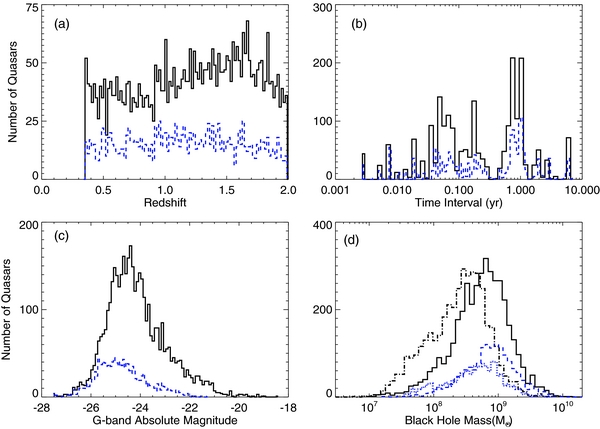
Figure 1. Basic properties of our sample. (a) Redshift. We select the redshift range of [0.36, 2] to keep the Mg ii line in the observing window of SDSS. (b) Time interval between multiple observations of the quasars. (c) Absolute magnitudes. (d) BH mass distribution. For (a), (b), and (c), the black (solid) lines are for the whole sample, while the blue (dashed) lines are for the S/N pixel−1 >10 subsample. For (d), the black (solid and dash-dotted) lines show the distribution of BH masses for the whole sample, while the blue (dashed and dotted) lines are for the high-S/N subsample. The solid and dashed lines are based on Mg ii widths (Shen et al. 2011b), while the dash-dotted and dotted lines show lower limits on the BH masses derived from their bolometric luminosities (Shen et al. 2011b) assuming that the bolometric luminosities are 50% of their Eddington luminosities. We assume that these BH masses are the secondary masses in a BH binary in our working scenario.
Download figure:
Standard image High-resolution imageIn Figure 1(d), the black (solid and dash-dotted) lines are BH mass distributions for the 4047 quasars in the whole sample (157 AGNs do not have available BH masses; they are assigned the median BH mass), while the blue (dotted and dashed) lines are for the high-S/N subsample (six of which do not have BH masses). We present two estimates of the BH mass. The solid and the dashed lines represent BH masses measured from the Mg ii broad-line widths from Shen et al. (2011b). They range from 107 M☉ to 1010.5 M☉ and are peaked at 108.65 M☉ (or 108.9 M☉) for the whole sample (high-S/N subsample). Taking the BH masses at face value together with the bolometric luminosities of these quasars (Shen et al. 2011b), the Eddington ratios ( ) have a median value of ∼0.25 while ranging from 0.02 to 2.7. The dash-dotted and dotted lines are lower limits on the BH mass derived from the bolometric luminosities (Shen et al. 2011b), assuming that the bolometric luminosity of each quasar is 50% of its Eddington luminosity. They range from 106.3 M☉ to 109.8 M☉ and are peaked at 108.3 M☉ (or 108.7 M☉) for the whole sample (high-S/N subsample).
3. CROSS-CORRELATION ANALYSIS
We are searching for a change in velocity in the Mg ii line linked to orbital motion in a sub-parsec BH binary. Note that the SDSS measures a redshift for every quasar at every epoch as well. In principle, we could use these redshift measurements to find cases of large radial velocity shifts. However, the SDSS redshift measurements have a larger dispersion from one epoch to the next than our method. Therefore, we use a single redshift for each quasar to move the spectra to the rest frame. All the following analyses are performed in the rest frame of the quasar.
Next, we must isolate the broad emission line from the continuum of the quasar. We find that variability in the quasar continuum can significantly decrease the sensitivity of the cross-correlation to the broad-line velocity shift. We fit the continuum with a fifth-order polynomial in each epoch. We prefer this to a power law because in some spectra the blue end of the continuum drops significantly due to an artifact, making it impossible to fit with a single power law. In fitting the continuum, we mask all the main emission lines and the 2σ wavelength regions around the centroids in the range from 1000 Å to 7300 Å (the centroid wavelengths and widths are from Vanden Berk et al. 2001, Table 2), namely, O vi (1000–1070 Å), Lyα (1142–1290 Å), Si iv (1389–1411 Å), C iv (1526–1572 Å), C iii] (1892–1926 Å), Mg ii (2770–2826 Å), Hγ (4318–4364 Å), Hβ (4810–4912 Å), [O iii] (4928–5038 Å), He i (5800–6000 Å, 7000–7200 Å) and Hα (6300–6800 Å). We subtract the fitted continuum to expose the Mg ii broad lines. One example is shown in Figure 2(a).
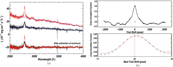
Figure 2. Example of the analysis of SDSS J095656.42+535023.2. (a) Polynomial fitting and subtraction of the continuum. The black and red lines on the upper part of the figure show the spectra of SDSS J095656.42+535023.2 at two epochs with a 6.16 yr separation. The blue lines are the fitted continuum. Spectra after continuum subtraction are shown on the bottom of the figure. (b) Cross-correlation function and peak hunting. The upper panel shows the cross-correlation at different trial shifts in pixels. The lower panel is zoomed in on 20 pixels at the peak region of the cross-correlation function. The two vertical dashed lines mark the position of the peak. The width of 1.7 km s−1 is the uncertainty in the peak reported by the Gaussian fitting. The resolution, i.e., the interval between two neighboring pixels (open square dots), is 17.3 km s−1. The best trial shift is marked with a red star on the upper panel.
Download figure:
Standard image High-resolution imageWe then cross-correlate the continuum-subtracted spectra from the two epochs, using all data in the wavelength range λ = 1700–4000 Å. We weight the flux in each pixel with its inverse variance from the SDSS observation, which efficiently prevents bad pixels from confusing our analysis. We calculate the cross-correlation at various trial velocity shifts:
where a and b are the spectra from the two epochs and D is the trial delay. The spacing of the trial delays is 17.3 km s−1, one-fourth of the SDSS spectral resolution.
Finally, we look for the peak in the cross-correlation function and define the corresponding trial velocity shift as our "best" measurement of velocity shift. The method we use to find the peak in the cross-correlation function is adapted from the SDSS III (BOSS) pipeline (Bolton et al. 2012), which measures centroids of peaks using a Gaussian fit around the minimum χ2. The peak cross-correlation values we find are equivalent to the maximum value in most cases, but in some extreme cases where there are offset local fluctuations sitting on the "true" peak, this Gaussian fitting method behaves better. In general, the uncertainty returned from the peak fitting is small (<20 km s−1), and thus much smaller than our systematic uncertainties (Section 4.1). An example of our cross-correlation and peak hunting is shown in Figure 2(b).
We mainly focus on the spectral region directly surrounding Mg ii (2700–2900 Å), where the strongest cross-correlation signal can be found. However, we are throwing away real information in the weaker broad emission lines such as Fe ii, which are found throughout the rest-frame near-UV spectrum. Thus, we also perform a wider cross-correlation over the region between 1700 Å and 4000 Å(Section 4.1). Using two wavelength regions allows us to remove many false positives that come from the narrow Mg ii considered alone.
4. RESULTS: SMBH BINARY CANDIDATE SELECTION
We measured broad-line velocity shifts for all of the 4204 quasars in our sample, and their distribution is shown in Figure 3. Since most of the quasars have very short time intervals between observations, their velocities will not change even if they harbor binary BHs. Therefore, the width of this histogram represents the typical errors incurred from noise in the data, sky subtraction and wavelength calibration errors, the finite width of the broad lines, and intrinsic variability in broad emission or absorption line shape. In fact, when we directly compare the ΔV (velocity shift) distribution of quasars with time baselines greater than or less than 2 weeks, the two distributions are consistent (at 69% significance level with a K-S test). The distribution of ΔV for all the 4204 quasars is peaked at zero, and its width is σ = 101 km s−1. In practice, we find that spectra with low S/N confuse our cross-correlation procedure, so we construct a high-S/N sample of 1523 objects with S/N pixel−1 > 10 to focus on the most reliable cross-correlation measurements. The distribution of measured velocity shifts in the high-S/N sample is shown in Figure 3. We get a histogram width of σ ≈ 82 km s−1 for this subsample, and accordingly we set 3.4σ ∼ 280 km s−1 as the lower limit for "significant velocity drifts" such that we expect <1 false positive detection in the high-S/N sample. However, we also insist that the cross-correlation measured from the Mg ii region alone be consistent within 1σ of that measured over the entire spectral region. By comparing the cross-correlations of the two regions, we are able to remove apparent shifts that are due to some small errors in sky subtraction, for instance.
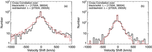
Figure 3. Measured velocity change of the broad line region for: (a) the whole sample where the width of the distribution is ∼101 km s−1 with cross-correlation over the whole wavelength range [1700 Å, 4000 Å], and is ∼126 km s−1 with cross-correlation over the wavelength range near Mg ii [2700 Å, 2900 Å]; and (b) the S/N pixel−1 >10 subsample, where the width of the distribution is ∼82 km s−1 with cross-correlation over both the [1700 Å, 4000 Å] and the [2700 Å, 2900 Å] ranges.
Download figure:
Standard image High-resolution imageIn the end, we pick our final list of candidates from the high-S/N sample with the following criteria:
Velocity shifts measured with the two methods (cross-correlating the whole spectral range or only the Mg ii line) should satisfy: (1) at least one of the two measurements is larger than 280 km s−1; (2) the difference between them is less than 1σ or 82 km s−1; (3) the error in the cross-correlation fit is <100 km s−1.
Seven objects obey these criteria. The selected candidates are described in Table 1. One of our final candidates (SDSS J095656.42+535023.2) comes from a plate flagged as "bad." This flag reflects the very poor seeing conditions and bright sky when the data were taken, and it may lead to large spectrophotometric uncertainty. However, most of the spurious features are introduced in the red end of the spectrum, far from the Mg ii line. We thus believe that our polynomial continuum fit will account for any remaining flux calibration issues in this target. According to these BH masses and the measured accelerations, the candidate SMBH binaries are expected to have separations of 0.01–0.1 pc at maximum.
Table 1. Selected Candidates
| SDSS ID | z | Mabs | log10MBH | Δt | ΔV1 | ΔV2 | Error | rmax | Last Observation |
|---|---|---|---|---|---|---|---|---|---|
| (M☉) | (yr) | (km s−1) | (km s−1) | (km s−1) | (pc) | ||||
| (1) | (2) | (3) | (4) | (5) | (6) | (7) | (8) | (9) | (10) |
| J032223.02−000803.5 | 0.62 | −22.8 | 8.2827 | 0.9123 | 780 | 760 | 0.22 | 0.032 | 10-20-2001 |
| J002444.11+003221.4* | 0.40 | −24.3 | 9.5618 | 0.2301 | 328 | 380 | 2.76 | 0.102 | 12-22-2000 |
| J095656.42+535023.2b + m* | 0.61 | −23.1 | 8.2944 | 6.1589 | 360 | 300 | 1.74 | 0.127 | 03-05-2008 |
| J161609.50+434146.8m | 0.49 | −22.8 | 8.1696 | 0.2000 | 330 | 250 | 5.10 | 0.021 | 06-18-2002 |
| J075700.70+424814.5 | 1.17 | −24.7 | 9.1311 | 0.0192 | 310 | 290 | 2.12 | 0.020 | 11-28-2000 |
| J093502.54+433110.7m | 0.46 | −25.6 | 9.3425 | 0.9452 | 290 | 270 | 2.10 | 0.181 | 01-31-2003 |
| J004918.98+002609.4* | 1.94 | −26.1 | 9.3148 | 0.2767 | −260 | −290 | 5.65 | 0.096 | 01-04-2001 |
Notes. (1) Object name in the SDSS catalog. (2) Redshift of the object from the SDSS catalog (Bolton et al. 2012). (3) Absolute g-band magnitude. (4) BH mass of the object measured from the Mg ii widths (Shen et al. 2011b). (5) The time interval between multiple observations. (6) The velocity shift of Mg ii measured by cross-correlation over the whole wavelength range [1700 Å, 4000 Å]. (7) The velocity shift of Mg ii measured by cross-correlation over the wavelength range near Mg ii [2700 Å, 2900 Å]. (8) The uncertainties of velocity shifts reported from peak hunting of cross-correlation functions. (9) The upper limit for the separation of the SMBH binary assuming a mass ratio of q = 1. The true separations are equal to these values only when the observer sits at the ideal position for watching velocity drifts: an edge-on orbit with the secondary BH just intersecting the line connecting the primary BH and the observer. (10) The date when the last SDSS observation of the quasar was taken, in the format of MM-DD-YYYY. * The more reliable candidates that pass the test cross-correlation over [1700 Å, 3800 Å] (see Section 4.1). m: for these quasars, one of the two epoch spectra has a "marginal" plate quality flagged in SDSS platelist. These plates get the "marginal" flag because either the minimum S/N of all the fibers is smaller than 15.0 or the number of exposures is smaller than 3. b: one of the two epoch spectra has a "bad" plate quality flag. This flag reflects the very poor seeing conditions and bright sky when the data were taken, and may lead to large spectrophotometric uncertainty. However, for this candidate, most of the spurious features are introduced in the red end of the spectrum, far from the Mg ii line. b+m: one of the two epoch spectra has a bad plate quality flag, while the other has a marginal flag.
Download table as: ASCIITypeset image
Noting that most of the sources have velocity shifts very close to our limit, we consider seven as an upper limit to the total number of detections in our sample. Interestingly, most of our candidates have z < 1. We suspect that this is due to the increasing difficulties of working in the red. The distribution of BH masses is quite similar to that of the whole sample. The numbers are small, but we find no abnormal spectral properties among these seven candidates. For instance, their SDSS colors (e.g., g − i) do not seem atypical for QSOs in this redshift range, as may be expected for a circumbinary disk (e.g., Syer & Clarke 1995; Gültekin & Miller 2012; Rafikov 2013).
Since the velocity shifts in the Mg ii broad lines are small compared with the line widths, in Figure 4 we plot the ratio of the spectra at the two epochs for each candidate, at wavelengths around Mg ii and Hβ (if present). These ratio spectra nicely highlight the velocity shifts via "bumps" or "valleys" around the line peaks. We clearly see such features in the ratio spectra of SDSS J032223.02−000803.5, SDSS J002444.11+003221.4, SDSS J095656.42+535023.2, SDSS J161609.50+434146.8, and SDSS J093502.54+433110.7. One target, SDSS J093502.54+433110.7, is in common with Shen et al. (2013).

Figure 4. Ratio of spectra at two epochs of the candidate SMBH binaries. The black solid lines show ratios of Mg ii broad lines, while the red solid lines show ratios of Hβ lines for comparison. Zero velocity lies at the rest frame of Mg ii and Hβ lines. The horizontal dashed lines show the approximate average levels of the ratio spectra far from the emission lines. Five of the seven candidates show "bumps" and "valleys" around the line peaks in both Mg ii and Hβ, consistently indicating the presence of velocity shifts in these quasars. The two arrows on the x-axis mark the velocity range where we perform cross-correlation of the Mg ii lines.
Download figure:
Standard image High-resolution imageWhile using the cross-correlation of two spectral regions effectively removes spurious targets, it also may remove some real targets. Thus, for completeness, in Table 2 we list all 64 targets that are recovered with velocity shifts larger than 280 km s−1 by the Mg ii cross-correlation alone, for future more detailed follow-up. Note that none of these targets come from a "bad" plate, although a few are from marginal plates as indicated. However, given the many uncertainties remaining in selecting these targets, we will consider seven objects as an upper limit on the true number of detected binary systems in our sample for the purposes of discussion.
Table 2. Long List of Candidates by Mg ii Cross-correlation Alone
| SDSS ID | z | Mabs | log10MBH | Δt | ΔV1 | ΔV2 | Error | rmax | Last Observation |
|---|---|---|---|---|---|---|---|---|---|
| (M☉) | (yr) | (km s−1) | (km s−1) | (km s−1) | (pc) | ||||
| (1) | (2) | (3) | (4) | (5) | (6) | (7) | (8) | (9) | (10) |
| J104315.10+312313.7m | 1.94 | −26.2 | 8.1240 | 0.1288 | −17 | −1863 | 2.71 | 0.006 | 03-01-2005 |
| J004052.14+000057.3 | 0.41 | −23.1 | 9.3988 | 1.2822 | −207 | −1501 | 4.89 | 0.097 | 12-18-2001 |
| J013418.19+001536.8 | 0.40 | −24.3 | 7.9043 | 1.0493 | 103 | 1050 | 9.98 | 0.019 | 10-21-2001 |
| J212639.96-065555.5m | 1.34 | −24.4 | 8.3162 | 0.0603 | 0 | −916 | 1.13 | 0.008 | 10-18-2001 |
| J111045.38+042142.7b | 0.77 | −24.2 | 8.1932 | 0.0082 | −17 | −880 | 5.44 | 0.003 | 03-23-2002 |
| J110539.65+041448.3b | 0.44 | −23.9 | 8.2472 | 0.0082 | 103 | 862 | 3.59 | 0.003 | 03-23-2002 |
| J232801.46+001705.0m | 0.41 | −22.2 | 8.8313 | 1.0466 | −120 | 845 | 8.03 | 0.061 | 10-18-2001 |
| J120142.24-001639.9b | 1.99 | −26.2 | 9.0953 | 0.7315 | −34 | 811 | 4.22 | 0.070 | 01-21-2001 |
| J034512.62+002245.9 | 0.41 | −22.2 | 8.8401 | 1.0685 | 103 | 786 | 8.62 | 0.064 | 10-19-2001 |
| J032223.02-000803.5 | 0.62 | −22.8 | 8.6694 | 0.9123 | 776 | 759 | 0.22 | 0.050 | 10-20-2001 |
| J002311.06+003517.5 | 0.42 | −21.3 | 8.3932 | 0.2301 | 69 | 698 | 7.09 | 0.019 | 12-22-2000 |
| J031830.60+011023.9m | 0.51 | −22.5 | 7.8357 | 1.2740 | 69 | 690 | 1.61 | 0.024 | 01-12-2002 |
| J081931.49+450801.5m | 1.88 | −25.7 | 8.6771 | 0.6794 | 155 | 684 | 7.65 | 0.046 | 10-25-2001 |
| J015454.88+004044.0m | 1.65 | −25.8 | 8.1363 | 0.8986 | 103 | 670 | 2.61 | 0.028 | 10-17-2001 |
| J002444.11+003221.4 | 0.40 | −24.3 | 9.3974 | 0.2301 | 604 | 660 | 2.77 | 0.062 | 12-22-2000 |
| J025331.93+001624.8m | 1.83 | −25.3 | 8.7330 | 0.9836 | 0 | 655 | 3.60 | 0.060 | 09-23-2001 |
| J230745.14-004542.7 | 1.84 | −25.3 | 8.4820 | 2.9397 | 34 | −638 | 4.91 | 0.078 | 09-02-2003 |
| J025156.31+005706.4m | 0.47 | −22.7 | 8.3595 | 0.8329 | 51 | −621 | 6.99 | 0.037 | 09-23-2001 |
| J135831.39+010339.2 | 0.41 | −22.8 | 8.8752 | 0.8247 | 17 | 621 | 2.92 | 0.066 | 02-02-2001 |
| J140140.44+325116.7m | 0.40 | −21.6 | 8.4292 | 0.1781 | −34 | 608 | 3.04 | 0.019 | 03-21-2007 |
| J115115.38+003827.0b | 1.88 | −26.5 | 8.3378 | 0.7699 | −51 | 604 | 1.78 | 0.035 | 02-03-2001 |
| J105014.02+275230.3 | 1.71 | −25.5 | 9.1812 | 0.0712 | −138 | −586 | 5.36 | 0.028 | 04-01-2006 |
| J011310.39-003133.3 | 0.41 | −22.4 | 8.3847 | 1.1178 | −172 | 552 | 5.30 | 0.046 | 10-20-2001 |
| J025316.45+010759.8m | 1.03 | −24.3 | 8.7330 | 0.9836 | 17 | −533 | 0.99 | 0.066 | 09-23-2001 |
| J075543.68+421146.0 | 0.42 | −22.4 | 8.0433 | 0.0192 | 34 | 519 | 3.19 | 0.004 | 11-28-2000 |
| J105417.14+241326.1 | 1.97 | −26.4 | 8.4642 | 0.0493 | 86 | 484 | 7.43 | 0.011 | 12-17-2006 |
| J015638.55+131757.8m | 1.98 | −26.3 | 8.1363 | 0.0630 | 103 | −483 | 9.66 | 0.009 | 12-22-2000 |
| J163905.16+142326.4 | 1.00 | −24.0 | 9.3655 | 1.0192 | 276 | 467 | 5.14 | 0.149 | 06-21-2006 |
| J144426.04-010546.0 | 0.56 | −22.9 | 9.1813 | 2.0521 | 69 | −465 | 2.17 | 0.171 | 05-17-2002 |
| J082214.83+431702.0m | 0.97 | −23.8 | 8.8360 | 0.6794 | 51 | −455 | 4.81 | 0.067 | 10-25-2001 |
| J145126.16+032643.4b | 0.48 | −23.1 | 8.7074 | 0.0438 | −51 | −455 | 3.46 | 0.015 | 05-16-2001 |
| J104913.85+221831.7 | 1.98 | −25.6 | 8.6655 | 0.0493 | −224 | −450 | 7.15 | 0.015 | 12-17-2006 |
| J002411.66-004348.1m | 1.79 | −26.2 | 8.7239 | 1.1534 | 0 | 444 | 7.29 | 0.078 | 10-21-2001 |
| J084119.42+171527.5 | 1.75 | −25.1 | 8.5174 | 0.0082 | 707 | 428 | 1.95 | 0.005 | 12-07-2005 |
| J151051.34-010906.3 | 1.76 | −25.5 | 9.2923 | 2.0247 | 17 | 414 | 2.89 | 0.205 | 05-10-2002 |
| J014209.72−002348.4 | 1.35 | −24.4 | 8.7042 | 1.1370 | −759 | −414 | 1.80 | 0.078 | 10-21-2001 |
| J114924.77−010010.3b | 1.13 | −24.5 | 8.4314 | 0.7699 | −189 | −396 | 6.27 | 0.048 | 02-03-2001 |
| J033211.85+002430.8 | 0.51 | −22.1 | 8.6316 | 0.1890 | 17 | −379 | 4.62 | 0.031 | 12-01-2000 |
| J230654.00−001605.6 | 0.56 | −22.9 | 8.8690 | 2.9918 | −69 | 379 | 4.03 | 0.160 | 09-02-2003 |
| J082012.62+431358.4m | 1.07 | −24.8 | 8.5195 | 0.6794 | 86 | 378 | 2.61 | 0.051 | 10-25-2001 |
| J004403.47+151200.0 | 1.78 | −25.6 | 9.2250 | 0.1836 | −86 | 374 | 3.91 | 0.060 | 12-01-2000 |
| J003451.86−011125.7 | 1.84 | −25.6 | 8.8775 | 1.2822 | −34 | −362 | 4.28 | 0.108 | 12-18-2001 |
| J020646.97+001800.6 | 1.68 | −25.5 | 9.0745 | 0.1781 | −51 | 362 | 2.78 | 0.051 | 11-29-2000 |
| J091621.10+012020.8m | 2.00 | −26.3 | 9.2819 | 0.0712 | 69 | −362 | 2.99 | 0.041 | 02-15-2001 |
| J163359.76−004512.6 | 1.24 | −24.2 | 8.8806 | 0.0685 | 69 | −349 | 3.73 | 0.026 | 06-01-2000 |
| J014415.12−002349.8 | 1.71 | −25.4 | 9.5618 | 1.1370 | −51 | 345 | 0.91 | 0.230 | 10-21-2001 |
| J124502.76+380514.2 | 1.05 | −24.9 | 8.8668 | 0.7589 | 86 | −345 | 5.57 | 0.084 | 02-06-2006 |
| J150638.54+573459.1 | 0.56 | −23.8 | 8.6990 | 0.0630 | 0 | −343 | 1.44 | 0.020 | 06-19-2001 |
| J164535.42+362712.3b | 1.81 | −26.0 | 8.0411 | 1.0219 | 34 | −340 | 8.91 | 0.038 | 05-23-2003 |
| J080915.74+273830.3b + m | 1.80 | −25.5 | 8.4768 | 0.1425 | −86 | −337 | 7.88 | 0.024 | 01-31-2003 |
| J161052.15+442421.3m | 1.23 | −24.4 | 8.1199 | 0.2000 | 51 | −334 | 1.21 | 0.019 | 06-18-2002 |
| J153111.83+442354.6 | 1.14 | −24.7 | 8.3325 | 0.0055 | 69 | −329 | 8.81 | 0.004 | 07-13-2002 |
| J025257.18−010220.9 | 1.25 | −24.2 | 8.7452 | 0.1671 | −17 | 318 | 2.47 | 0.036 | 11-29-2000 |
| J002028.35−002915.0 | 1.93 | −25.3 | 8.3291 | 0.2301 | −224 | 310 | 3.10 | 0.026 | 12-22-2000 |
| J163523.71+134036.6 | 1.81 | −25.3 | 8.7050 | 0.0822 | 17 | 310 | 2.06 | 0.024 | 06-21-2006 |
| J215213.51−074224.9b + m | 0.95 | −24.3 | 8.3290 | 0.0658 | 0 | 310 | 6.56 | 0.014 | 09-21-2001 |
| J102536.43+645242.9m | 1.37 | −24.9 | 8.3168 | 0.0438 | 224 | 307 | 3.21 | 0.011 | 01-21-2001 |
| J095656.42+535023.2b + m | 0.61 | −23.1 | 7.9160 | 6.1589 | 362 | 303 | 1.74 | 0.086 | 03-05-2008 |
| J014905.16+005925.3 | 1.00 | −24.2 | 8.5702 | 1.1205 | −69 | −299 | 5.93 | 0.078 | 10-20-2001 |
| J155631.51+080051.8m | 1.92 | −25.8 | 8.6527 | 1.7288 | 241 | −294 | 4.00 | 0.108 | 05-04-2006 |
| J020527.77−005747.6 | 1.24 | −24.7 | 9.0239 | 0.1781 | −86 | 293 | 5.66 | 0.053 | 11-29-2000 |
| J075700.70+424814.5 | 1.17 | −24.7 | 8.9236 | 0.0192 | 310 | 293 | 2.12 | 0.016 | 11-28-2000 |
| J085626.71+570444.7 | 1.52 | −24.6 | 8.9563 | 0.1151 | 0 | −293 | 7.97 | 0.039 | 02-02-2001 |
| J004918.98+002609.4 | 1.95 | −26.1 | 7.9173 | 0.2767 | −258 | −289 | 5.65 | 0.019 | 01-04-2001 |
Notes. (1) Object name in the SDSS catalog. (2) Redshift of the object from the SDSS catalog (Bolton et al. 2012). (3) Absolute g-band magnitude. (4) BH mass of the object measured from the Mg ii widths (Shen et al. 2011b). (5) The time interval between multiple observations. (6) The velocity shift of Mg ii measured by cross-correlation over the whole wavelength range [1700 Å, 4000 Å]. (7) The velocity shift of Mg ii measured by cross-correlation over the wavelength range near Mg ii [2700 Å, 2900 Å]. (8) The uncertainties of velocity shifts reported from peak hunting of cross-correlation functions. (9) The upper limit for the separation of the SMBH binary assuming a mass ratio of q = 1. The true separations are equal to these values only when the observer sits at the ideal position for watching velocity drifts: an edge-on orbit with the secondary BH just intersecting the line connecting the primary BH and the observer. (10) The date when the last SDSS observation of the quasar was taken, in the format of MM-DD-YYYY. m: for these quasars, one of the two epoch spectra has a "marginal" plate quality and the other epoch has "good" plate quality flagged in SDSS platelist. Plates get the "marginal" flag because either the minimum S/N of the fibers is smaller than 15.0 or the number of exposures is smaller than 3. b: one of the two epoch spectra has a "bad" plate quality flag, while the other has a "good" flag. The "bad" flag reflects the very poor seeing conditions and bright sky when the data were taken, and may lead to large spectrophotometric uncertainty. However, for this candidate, most of the spurious features are introduced in the red end of the spectrum, far from the Mg ii line. b+m: one of the two epoch spectra has a "bad" plate quality flag, while the other has a "marginal" flag.
4.1. Uncertainties
There are various sources of uncertainties in our measurements, including wavelength calibration, sky subtraction, continuum subtraction, and cross-correlation errors. The statistical error reported by the cross-correlation procedure is typically <20 km s−1, with only ∼3% of objects having uncertainties greater than 100 km s−1. We further create mock spectra using the SDSS variance arrays and perform input–output tests of our cross-correlation analysis. We recover a very narrow distribution of uncertainties in our output velocity shifts (<34 km s−1 in all cases). Random errors alone cannot explain the width of the velocity distribution that we observe.
One source of systematic uncertainty comes from our choice of wavelength region for the cross-correlation. While the cross-correlation over the whole range [1700 Å, 4000 Å] helps us remove some false-positives, it also introduces further potential sources of uncertainty. For instance, absorption from the Ca H+K lines around the 4000 Å break, or errors in sky subtraction, may confuse our technique. As a sanity check, we did another set of cross-correlations for the seven candidates over [1700 Å, 3800 Å] to exclude Ca H+K absorption lines. Only three of the seven candidates (SDSS J002444.11+003221.4, SDSS J095656.42+535023.2, SDSS J004918.98+002609.4) survive this test. These are our three most reliable candidates. As a result, we consider seven as an upper limit in what follows.
There are many other contributions to the velocity uncertainties. The first effect is uncertainties in sky subtraction, as already discussed. Second, intrinsic changes in the quasar continuum may be a source of uncertainty. When we change the spectral region used for the continuum fit, the output velocities can change by tens of km s−1, showing that our continuum fitting also contributes to the error budget. Third, there is irreducible scatter from temporal variations in the broad lines themselves (e.g., Sergeev et al. 2007; Gezari et al. 2007; Decarli et al. 2013). We do not yet know the full range of velocity shifts resulting from line-shape variability. Therefore, we cannot take the observed distribution of velocity offsets and infer anything about the binary population below our detection threshold, as in Badenes & Maoz (2012).
5. EXPECTED NUMBER OF OBSERVABLE CANDIDATES
We define the observability of an SMBH binary system to be the probability for the binary to have a projected velocity drift above our detection threshold as defined in Section 4. In this section, we estimate the observability of BH binaries given the distribution of BH masses and time intervals in the sample, and two different assumptions about the BH merging process. For simplicity, we start with the assumption that all the quasars are in a tight binary phase, with only one accreting BH. We further assume that the quasar activity that we observe is associated with the secondary BH. Simulations do find increased accretion rates onto the secondary from a circumbinary disk due to the proximity of the secondary to the ambient gas (Cuadra et al. 2009). Therefore, we assume that the BH masses measured by Shen et al. (2011b) shown in Figure 1(d) are the masses of the secondary BHs. Note that since the quasars are quite luminous, they are most likely found in comparable-mass binaries under these assumptions.
The observability of SMBH binaries depends on the following parameters. (1) The total BH mass [MBH, (1 + q)/q × measured BH mass], mass ratio (q = Msecondary/Mprimary), and separation of the two BHs (r), which together determine the acceleration of the secondary. (2) The time interval (Δt) between multiple observations of the same quasar. (3) The projection of the orbit on the sky. For our sample, we know the time interval between observations, and we assume that the total BH mass of the binary is known. We assume that the binary inclination and phase are oriented randomly on the sky with respect to the observer. The only free parameters are the mass ratio q and separation r of the binary BHs.
This section will proceed as follows. In Section 5.1 we calculate the observability of a BH binary with a given mass, mass ratio, separation, observing time interval and orientation. Then we randomly sample the inclination and the phase of the binary and calculate the observability of each quasar in our sample utilizing the BH mass and observing time interval. The sum of observabilities for all of the quasars gives us the total expected number of observable candidates (Nobs). We will derive the dependence of Nobs on mass ratio by fixing the orbital separation and on separation by fixing the mass ratio.
We then relax the assumption that the BH binaries spend their whole life at a fixed separation. In Section 5.2, we theoretically calculate the residence time (tres) as a function of radius of the BH binaries in the scenario of gas-assisted evolution at sub-parsec scales (r ≲ 0.1 pc). Since the probability to find a quasar at a given radius is proportional to the residence time of the BH binary at that radius [dt = (tres/r)dr], the detectability of one SMBH binary system is then the integral of the detectability over radius, weighted by the residence time:
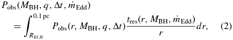
where Δt is the time interval between observations of one AGN, RBLR is the size of the BLR (Shen & Loeb 2010),
and  is the Eddington accretion rate ratio. The RBLR scaling is derived from local reverberation mapping campaigns (e.g., Bentz et al. 2009, 2013), which find that RBLR∝L1/2. Note that we are extrapolating this relation into the redshift and luminosity range of our observed quasars. The probability Pobs(MBH, q, Δt) is evaluated for each object in our sample using its own MBH and Δt while assuming that all of the objects have the same mass ratio q. The sum of Pobs over all of the objects is then the total expected number of observable sources (Nobs). We discuss our results and their sensitivity to the parameters in Section 5.3.
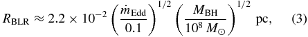
A major uncertainty in the detectability comes from the size of the BLR, RBLR. As the two BHs get closer than RBLR, the BLR will envelope both of the BHs such that the broad emission lines are no longer sensitive to the orbital motion of a single BH (Shen & Loeb 2010). The BLR of the secondary BH could also suffer tidal truncation at the Roche lobe surface as the binary gets tighter (Montuori et al. 2011) and may be totally destroyed when the binary separation is comparable to RBLR. Therefore, we take RBLR as a lower limit of our integration in Equation (2). Our estimates of observability are very sensitive to the assumed RBLR because the smallest separations contribute most to the observability. A slightly larger RBLR leads to a significant decrease in our chances of detecting orbital motion of the binaries. From reverberation mapping, the expected BLR size for a single BH of 108 M☉ (or 109 M☉) is about 0.022 pc (or 0.07 pc) assuming the Eddington ratio of the QSO to be ∼0.1 (Shen & Loeb 2010).
We note, however, that tidal truncation may change our results. Based on the locally optimally emitting cloud model of the BLR (Baldwin et al. 1995), the Mg ii emitting region is quite broad (Korista & Goad 2000) and would be observable even in a BLR 1/10 the fiducial assumed size. We could be more sensitive to SMBH binaries than the estimates in this section, if the BLR is more compact in tight binaries. In the future, we will use the C iii] line, which comes from a much more compact region (Wayth et al. 2005), to mitigate these uncertainties.
5.1. Observability at Fixed Separation and Binary Mass Ratio
Let us start with the observability of a BH binary Pobs for a given total mass MBH, mass ratio q, separation r, observing time interval Δt, and orientation on the sky. Note that the total mass MBH is equal to (1 + q)/q times the BH mass shown in Figure 1(d), since we assume that we are observing the secondary BH. Although simulations show that very high eccentricity may arise through binary–star interactions (e.g., Sesana et al. 2008; Sesana 2010; Preto et al. 2011; Khan et al. 2012) and binary–disk interactions (e.g., Armitage & Natarajan 2005; Cuadra et al. 2009; Roedig et al. 2011), the eccentricity of the binary orbit is highly uncertain. For simplicity, we assume zero eccentricity throughout, so that the intrinsic velocity of the secondary BH is
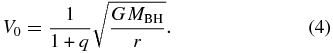
The observed velocity is Vobs = V0sin ϕcos θ, where ϕ and θ are the azimuthal and polar angle respectively, of the observer on the sphere centered on the BH binary. θ = 0 when the binary orbit is edge-on relative to the observer, and ϕ = 0 when the secondary (accreting) BH lies between the observer and the center of mass of the binary. If this quasar is observed twice with a time interval of Δt, then the drift in velocity of the secondary BH is

where  is the angular velocity.
If the observer has equal chances to be at any solid angle on this sphere, then ϕ is uniformly distributed in [0, 2π] and |cos θ| also has an equal chance to have any value between [0, 1] according to dΩ = cos θdθdϕ = d(sin θ)dϕ. Let us say that the smallest velocity drift we can measure is ΔVlim (ΔVlim = 340 km s−1 for our whole sample and ΔVlim = 280 km −1 for the high subsample). We now calculate the probability that |ΔVobs| exceeds the observational limit.
For a given cos θ, the probability of |ΔVobs| > ΔVlim, i.e.,

in the range ϕ ∈ [0, 2π], is
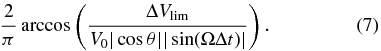
If we weight this value with the probability distribution of |sin θ| in the range [0, 1], the total probability becomes
where θmax satisfies ΔVlim/(V0|cos θmax||sin (ΩΔt)|) = 1.
We calculate the observability above for each object in our sample and sum them, which gives us the total number of candidates. The dependence of the total expected number of candidates on the mass ratio and separation of the BH binary are shown in Figures 5 and 6, respectively. In Figure 5 we fix the separation to be 0.1 pc and vary the mass ratio q from 0.01 to 1. The observability is moderately sensitive to the mass ratio. The expected number of observable sources increases by a factor of 10 as q decreases by a factor of 100. This sensitivity is mainly due to the dependence of the total BH mass MBH on q, as we assume that we observe the secondary BH. The number of observable candidates increases more steeply as the radius decreases (Figure 6), because the orbital velocity of the BHs is proportional to r−1/2. No BH binaries are observable if the separation gets larger than ∼0.3 pc for q = 1 (or ∼1 pc if q = 0.1). We do additional calculations at fixed separation while truncating the observability at RBLR for each object (dash-dotted and dotted lines in Figure 6). In Section 5.3 we will compare our number of candidates with the models in the scenario where all quasars live at a fixed separation forever.

Figure 5. Dependence of expected number of observable binaries (Nobs) on the mass ratio q of SMBH binaries at a fixed separation of 0.1 pc. The sensitivity mainly comes from the dependence of total BH mass on q, given an observed secondary BH mass.
Download figure:
Standard image High-resolution image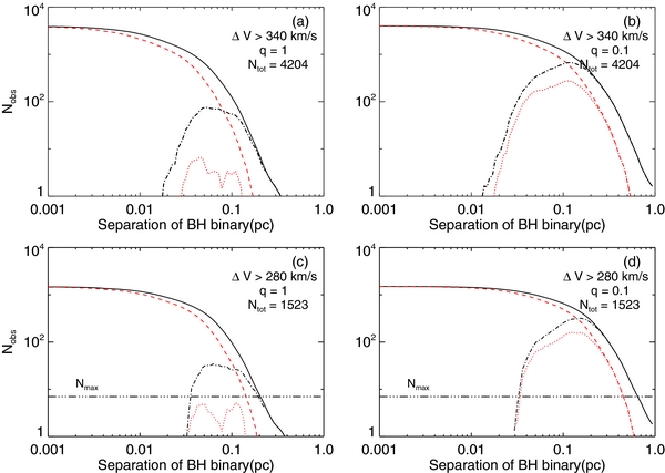
Figure 6. Dependence of the expected number of candidates (Nobs) on the separation of the SMBH binaries. (a) and (b) are for the whole sample with Ntot = 4204, and (c) and (d) are for the S/N pixel−1 > 10 subsample with Ntot = 1523. The black (solid and dash-dotted) lines utilize BH masses from broad-line width measurements, while the red (dashed and dotted) lines use the lower limits to the BH masses as estimated from the bolometric luminosity assuming an Eddington ratio  . The dash-dotted and dotted lines include truncation at RBLR in the calculations, while the solid and dashed lines do not. The horizontal lines in the lower panels are the upper limits from this experiment (N ⩽ 7).
Download figure:
Standard image High-resolution image5.2. Time Evolution of the SMBH Binary
We now calculate the second ingredient needed to compute Pobs using Equation (2)—the residence time tres as a function of the binary separation r for a given set of binary characteristics.
From Table 1, our candidate SMBH binaries are at separations of 0.01–0.1 pc or closer, well inside the regime of "the final parsec." As mentioned in the Introduction, there are many mechanisms proposed to overcome the final parsec problem. One of the most promising is tidal interaction of the binary with a circumbinary disk, naturally leading to the orbital decay of the binary, which loses its angular momentum to the disk (e.g., Haiman et al. 2009; Cuadra et al. 2009; Rafikov 2013). It is generally expected that a massive binary clears a cavity in a disk around itself so that the mass inflow onto its components is considerably suppressed compared to the mass accretion rate  far out in the disk. Mass accumulation at the inner edge of the disk caused by the tidal barrier modifies the disk structure over time and accelerates binary inspiral.
In this work we compute tres in the framework of this gas-assisted binary inspiral scenario. If we assume that all quasars are triggered by gas accretion at ∼0.1 pc and the inspiral of the central SMBH binaries is dominated by the interaction with a gas disk, then the probability of observing a pair at a given radius is just proportional to the residence timetres ≡ |dln r/dt)|−1. This time is obviously a function of the physical mechanism driving the orbital evolution of the binary. As a result, our observations in principle provide a way of constraining different inspiral mechanisms.
Our calculation of tres closely follows that in Rafikov (2013), which provides a recipe for computing the fully coupled, time-dependent binary+disk evolution and should be referred to for details. We start binaries of all masses at a semi-major axis of 0.1 pc, in a circumbinary disk with viscosity characterized by α = 0.1. We assume that in a radiation-pressure-dominated regime (which is valid at small separations) viscosity in the disk is proportional to the total (rather than the gas) pressure. The value of the mass accretion rate in the disk far from the binary  is normalized by the Eddington rate
  computed for the full binary mass and radiative efficiency of ε = 0.1. Evolutionary calculations are always started with a constant
  disk extending all the way into the initial binary orbit at 0.1 pc. Such an initial setup naturally arises if the gas that has fallen into the center of the galaxy circularizes outside the binary orbit and then viscously spreads inward. For simplicity our calculations ignore the issue of gravitational stability of the circumbinary disk at large separations, which is poorly understood at the moment (Goodman 2003; Rafikov 2009).
Rafikov (2013) has shown that the torque acting on the binary and driving its inspiral is set by  , the radius of influence rinfl out to which the binary torque has been propagated by the viscous stresses in the disk, and the degree of mass overflow across the orbit of the secondary, i.e., the fraction χ < 1 of
  that penetrates into the cavity and gets accreted by the binary components. The dependence on the latter is rather weak and the orbital evolution is similar to the no-overflow case as long as χ ≲ 0.2, which we assume to be the case in this work for simplicity. Of course, in practice some overflow is needed to power the observed quasar activity, so χ is not strictly zero.
The time dependence of the radius of influence is self-consistently computed by following the viscous evolution of the circumbinary disk torqued by the binary, as described in Rafikov (2013). In calculating rinfl we keep track of the different physical regimes in the disk at rinfl. This is important since rinfl can vary by orders of magnitude with respect to the binary semi-major axis in the course of its inspiral, allowing the opacity behavior and relative role of radiation pressure at rinfl to change over time. This self-consistent calculation favorably distinguishes our present calculation (and that in Rafikov 2013) from the self-similar solution of Ivanov et al. (1999) or the SMBH inspiral calculations in Haiman et al. (2009).
One particular aspect of the tres calculation that we wish to emphasize is that in many cases we find the system in so-called disk-dominated evolution, a regime when the "local disk mass"4Md = Σr2 at the inner edge of the disk (here Σ is the local surface density of the disk enhanced by the mass pileup near the cavity edge) is larger than the mass of the secondary Ms. This regime is often valid at the initial stages of evolution, especially for lower SMBH masses, because of the large starting semi-major axis of 0.1 pc that we adopt in this work. In this regime we follow conventional wisdom (Ward 1997; Haiman et al. 2009) and simply assume that the secondary passively follows viscous evolution of the disk, which is equivalent to setting tres = tν, where tν = r2/ν is the viscous time at the inner edge of the circumbinary disk, computed using the local value of viscosity ν and accounting for the possibility of mass pileup at the inner disk edge. As the binary orbit shrinks, the system inevitably transitions into the secondary-dominated regime, when Ms > Md. As soon as this happens, we let the disk respond viscously to the binary torque. On the other hand, Rafikov (2013) has shown that deep in the secondary-dominated regime (Md ≪ Ms) the evolution (or residence) time is given by

Thus, tres evaluated according to this formula becomes equal to tν only when Md = Ms/[6π(1 + q)], which is significantly less than Ms. The precise details of the transition between the disk- and secondary-dominated regimes are not well understood at the moment, so in this work we assume for simplicity that tres = tν for Md > Ms/[6π(1 + q)] and switches to the behavior predicted by Equation (9) only for Md < Ms/[6π(1 + q)]. This assumption makes the viscous evolution of the disk quite important and can potentially result in an overestimate of tres at intermediate separations (∼0.01–0.1 pc) by a factor of several. We cannot be more accurate in this regime without better understanding the regime when Md ∼ Ms.
In Figure 7 we show maps of tres computed according to the aforementioned prescription (Rafikov 2013) for several values of q and  . Several features of these maps are worth discussing. At high masses (and small separations) color contours turn into straight lines, which reflects the fact that in this regime the binary inspiral is determined by GW emission. In this case tres is simply given by

where RS ≡ 2GMBH/c2 is the Schwarzschild radius of the BH with the combined mass MBH. This timescale is very sensitive to MBH and r, as can be seen in Figure 7. However, the quasars used in our study almost never probe this part of the parameter space because the size of the BLR RBLR (shown by the dot-dashed line in tres maps) exceeds the maximum separation at which GW emission dominates for all masses. Thus, our quasars are in the regime when the disk torque dominates binary inspiral.
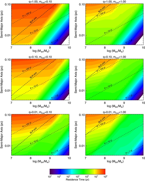
Figure 7. SMBH binary evolution driven by gas disks: color maps of residence time tres at various radii r for a range of BH masses. The value of tres is indicated by the color bar. Plots on the left (right) assume an Eddington accretion rate ratio ( ) of 0.1 (1.0). Plots on the top, center, and bottom assume that the mass ratio of the BH binary is 1, 0.1, and 0.01 respectively. Dashed lines are curves of constant orbital period (labeled), and the dot-dashed line is the RBLR given by Equation (3). See text for more details.
Download figure:
Standard image High-resolution imageFigure 7 also reveals some obvious trends with q and  . Lower q results in faster inspiral since for a lower-mass secondary the binary contains less angular momentum but the disk torque is relatively insensitive to q (see Rafikov 2013). Higher
  at a fixed MBH implies a circumbinary disk with higher surface density, which provides more torque, considerably accelerating the orbital evolution of the binary. Higher
  also extends the disk-dominated phase of the binary evolution. In particular, at low masses (and large separations) tres exhibits rather weak dependence on MBH, which is a result of the system evolving in a disk-dominated regime where the inspiral time is given by the local viscous timescale, which is only weakly dependent on MBH.
Quite important for our work is the relatively weak dependence of tres on separation in some cases, e.g., low  and relatively high q, which results in rather long tres for r ∼ 0.003–0.1 pc and increases the number of binaries in this range of r. This behavior is a result of two main factors. First, initially, when the system is in the disk-dominated regime, the inner parts of the disk around the binary are gas pressure dominated. Under these conditions the viscous timescale on which the binary orbit evolves in the disk-dominated case is a relatively weak function of r compared to the radiation-pressure-dominated case typical for high
  (Rafikov 2013), so that tres is quite long at
  pc.
pc.
Second, even after evolution switches to the secondary-dominated regime, binary inspiral is slow and is still not very sensitive to the separation (e.g., see the behavior of tres in Figure 8 of Rafikov (2013)). It is very important that here we self-consistently follow the time-dependent structure of the whole disk in the spirit of Ivanov et al. (1999). Previously, Haiman et al. (2009) found considerably faster binary evolution (lower tres) for the same MBH, r, etc., when employing the quasi-steady-state circumbinary disk solutions derived in Syer & Clarke (1995), which do not apply to real disks; see Ivanov et al. (1999) and Rafikov (2013) for details. The non-locality of the binary–disk coupling in the secondary-dominated regime (Rafikov 2013)—the fact that for a given value of  at the inner disk edge (equal to zero in the case of no overflow) the magnitude of the torque acting on the binary is set by the disk properties not at its inner edge, which is often radiation pressure dominated, but much farther out, at rinfl, where the disk is gas pressure dominated—is also very important for determining the residence time.
5.3. Results: Expected Number of Observable SMBH Binaries
In computing observability, we consider two basic scenarios for the BH binary: no temporal evolution, and radial migration via a gaseous accretion disk. From each, combined with our upper limit of seven candidates, we can infer something about the BH binary population in luminous z ≈ 1–2 QSOs. In the first scenario, all SMBH binaries live at fixed separation with no time evolution as we discussed in Section 5.1. The expected numbers of observable sources from our high-S/N subsample versus binary separation is shown in Figure 6. Comparison of this theoretical distribution with our observational upper limit (N ⩽ 7) rules out that all the ∼109 M☉ BHs that we observe at z ≈ 1–2 exist in binaries in the separation range of ∼[0.03, 0.2] pc. Binaries closer than 0.03 pc are not observable due to the truncation or destruction of the BLR, while binaries with r > 0.2 pc are not observable given the Δt distribution of our sample. We note that even this basic result is of cosmological interest. For instance, in the merger-tree models of Volonteri et al. (2003), many major mergers are expected in the massive halos that host our massive BHs between 1 < z < 2. We can rule out that the lifetime of the resulting tight binaries is comparable to the Hubble time in all cases (Section 7).
In the second scenario, the binaries evolve through a gas disk. With the residence time  calculated in the previous section (Section 5.2, Figure 7), the probability
  is evaluated according to Equation (2) for each object in our sample using its observed MBH and Δt and assuming that all of the objects have the same mass ratio q. The sum of Pobs over the objects is then the total expected number of observable sources (Nobs). As we discussed in Section 2, the virial masses of the secondary BHs shown in Figure 1(d) imply an
  distribution peaked at ∼0.25. For the first calculation of Nobs, we use tres in the case that
  and the virial BH masses. Then, to bracket the known large uncertainties in MBH measurements (e.g., Vestergaard & Peterson 2006; Shen et al. 2008), we also do the calculations assuming that
  and adopting MBH accordingly. In both of the calculations, we truncate the binary migration at RBLR for each object according to Equation (2), using the virial and Eddington-limited BH masses, respectively. We show the range of expected Nobs in our S/N pixel−1 >10 subsample for
  and q = 1, 0.1 in Table 3.
Table 3. Expected Number of Observable Sources in the S/N pixel−1 > 10 Subsample
 |
 | |
|---|---|---|
| q = 1.0 | 44 | 0.34 |
| q = 0.1 | 282 | 81 |
Notes. The four sets of numbers show the expected number of observable sources in our S/N pixel−1 > 10 subsample, adopting four sets of ( ) in the scenario of gas-assisted sub-parsec evolution of the SMBH binaries. We take the virial BH masses for the
  cases and Eddington-limited BH masses for the
  cases. For comparison, in the no-evolution case with r = 0.1 pc, we expect 40–98 sources for q = 1 and 498–655 sources for the unrealistic q = 0.1 case.
Download table as: ASCIITypeset image
If we adopt the most likely parameters  and q = 1, the final expected number of SMBH binaries in the high-S/N subsample is Nobs = 44. Comparison of this expectation with our seven candidates implies that <16% of quasars host SMBH binaries with r < 0.1 pc. A more extreme mass ratio of q = 0.1, which seems unlikely for the bulk of our sample, increases the expected Nobs by a factor of ∼6.4.
Note, however, that our results are very sensitive to the extrapolated RBLR–Lbol scaling relation, which is highly uncertain. Since our method is only sensitive to binaries that are less than ∼0.1 pc apart (see Figure 6), the final expected number of observable candidates is actually determined by the detectability within the range [RBLR, 0.1 pc]. Candidates in this range are the most massive BHs with the corresponding largest velocity drifts, so their BLR size is approaching ∼0.1 pc (e.g., RBLR ∼ 0.07 pc for 109 M☉ assuming  ). A slightly larger RBLR makes the valid range [RBLR, 0.1 pc] much narrower. We will test the sensitivity to RBLR quantitatively in Section 6.
The sensitivity of our results to  has two origins. First, the BH masses we use scale with
  given the observed luminosity. Second, the gas-assisted evolution of BH binaries depends on
  : in the lower
  case the circumbinary disk is less massive, meaning (1) more significant dominance of the secondary BH over the local disk (larger Ms/Md) and (2) less torque acting on the binary (which is proportional to
  ). These factors increase tres for RBLR < r < 0.1 pc in our scenario of the gas-assisted evolution, boosting the expected Nobs for lower
  .
.
Our results are also very sensitive to the details of the gas-assisted evolution model in the intermediate separation range [RBLR, 0.1 pc]. Evolutionary models where BH binaries spend a longer time in this radial range predict a larger number of observable sources Nobs. In our calculation of tres following Rafikov (2013) in Section 5.2, this separation range falls in the secondary-dominated regime, in which matter piles up outside the binary orbit and binary evolution is slow and is described by Equation (9). Faster orbital evolution in this separation range, as suggested by Haiman et al. (2009) based on the circumbinary disk solution by Syer & Clarke (1995), would result in a smaller number of detectable SMBH binaries. Thus, it should in principle be possible in the future to discriminate between the different evolutionary scenarios.
We restate that all the results in this study are based on the assumption of circular SMBH binary orbits for simplicity. The effects of eccentric orbits on SMBH binary detection are not certain due to the uncertainty of BLR physics. For an eccentric binary orbit (1) the individual BLRs around the SMBHs would either be truncated earlier during inspiral and thus more compact, making the velocity shifts easier to detect, or be tidally destroyed earlier, making a detection more challenging; and (2) larger velocity drifts characteristic for eccentric orbits would in principle allow us to sample a broader mass range of SMBHs relative to the circular orbits.
Another important mechanism that may solve the final parsec problem is that stars in a triaxial galaxy nucleus could continuously replenish the loss cone and drive subsequent inspiral evolution (Merritt & Poon 2004; Merritt & Vasiliev 2011). Merritt & Poon (2004) found that stars on chaotic (centrophilic) orbits in a triaxial galactic nucleus could refill the loss cone and feed the central BHs at quite a high rate and thus drive binary evolution at sub-parsec scales. Merritt & Vasiliev (2011) found that there exists a family of stellar orbits in triaxial galaxies called pyramid orbits. The angular momentum of stars can reach zero at the "corners" of the pyramid, at which point they are easily captured by the central BHs. The lifetime of the binary then becomes a function of the structure of the merged remnant (Khan et al. 2012) but may take billions of years. In this scenario, quasars could be ignited at any radius, since the lifetime of the quasar is likely much shorter than the inspiral timescale of the BH binaries. However, without more assumptions about the dynamical state of the galaxy centers to determine tres, we cannot easily predict the detectability of SMBH binaries in this scenario.
In the most pessimistic evolutionary scenario, the SMBH binaries stop spiraling inward due to depletion of stars and stall there forever. Quinlan (1996) did scattering experiments and found that the orbital decay of the binary stalls when most of the stars have been ejected, and this stalling separation is 0.01–1 pc depending on the mass and mass ratio of the BH binary. The stalling separation we extract from Quinlan (1996, see their Figure 7) is
For major mergers (q ∼ 1), the stalling radius is around ∼1 pc. If there is no subsequent driving mechanism and all binary BHs stall at ∼1 pc, our experiment would not be sensitive to any binary BHs according to Figure 6. With time baselines of only a few years, as probed here, we cannot hope to see radial velocity changes in parsec-scale binaries. However, as we will see in the next section, next-generation surveys could significantly increase the observability even in this scenario due to longer observing time intervals.
6. NEXT-GENERATION SURVEYS
As part of the BOSS (Schlegel et al. 2009; Dawson et al. 2013), 14,235 SDSS quasars, mostly in the redshift range 2.1 < z < 3.0, are being revisited with ∼10 yr time separations, with increasing numbers as the survey goes on. This provides a great opportunity to search for SMBH binaries using our cross-correlation methodology. We can use either C iii] or C iv to measure shifts in this sample. As discussed above, C iv may show many variations in line shape that have nothing to do with a binary companion but arise (for instance) in a disk wind (e.g., Proga et al. 2000). We believe that C iii] should be quite promising, however. To investigate the potential impact of the BOSS multi-epoch sample, as well as future surveys, we predict the observability of BH binaries as a function of time interval. Since the BH masses measured from C iv widths (currently available for 9002 of the 14,235 quasars; Shen et al. 2011b) are uncertain, we simply adopt the same mass distribution as our DR7 sample for the purpose of illustration.
As we discussed in Section 5.2, detectability depends on the evolutionary scenario of SMBH binaries at sub-parsec scales. In a scenario where circumbinary disks drive the inspiral of BH binaries following the tres distribution in Figure 7, the observability as a function of the time interval between observations of the same quasar is shown in Figure 8 (left panel for  , and right panel for
  ), where the star marks the upper limit on the detectability from our detection in the SDSS DR7 high-S/N subsample.
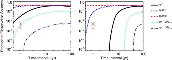
Figure 8. Observability of SMBH binaries in a next-generation survey assuming that at sub-parsec scales, the SMBH binary inspiral is driven by interactions with the accretion disks (see Section 5.2, Figure 7). Left:  . Right:
  . The solid (black), dash-dotted (blue), and dashed (red) lines are assuming a binary mass ratio of 1, 0.1, and 0.01, respectively, while all of them adopt the RBLR from Shen & Loeb (2010). The dotted (green) and dash-dotted (purple) lines increase the BLR size by a factor of two and three, respectively, just to show the sensitivity to values of RBLR of our results. The big asterisk marks our detection from the SDSS DR7 high-S/N subsample. If we reobserve all 105 SDSS quasars with time intervals of 10 yr, then we would expect ∼3 × 10⁴ binary detections if all quasars were equal-mass tight binaries, or ∼4 × 10⁴ for q = 0.1 tight binaries.
Download figure:
Standard image High-resolution imageAs before (see Section 5.3), the Eddington ratio  makes a big difference because (1) larger
  corresponds to smaller BH masses at a given luminosity, which leads to smaller velocity drifts at all separations, and (2) the time tres that BH binaries spend at intermediate separations is smaller for higher
  . The distribution of Eddington ratios likely lies between these two limits for the majority of sources (e.g., Shen et al. 2011b). For major mergers (q ∼ 1) with
  , we would expect ∼30% of the sources to show orbital motions for a time interval of ∼10 yr, which would correspond to a large number of targets in next-generation surveys (e.g., 1800 expected candidates from the BOSS QSO sample with multiple observations). Considering our constraints on the fraction of quasars that are triggered in a tight binary phase (<16%), the expected observability in the scenario above is ∼4.8%. However, this value drops to ∼1.6% if most sources are closer to
  . More extreme mass ratios would yield much higher observability, given the assumption that all the observed quasars are the secondary BHs, but to probe such low-mass ratios we likely would need to observe less luminous (lower-mass) QSOs. We should again caution that our predictions are very sensitive to the assumption of BLR size. As Figure 8 shows, the observability drops by a factor of ∼10 if we increase the BLR size by a factor of two. If we increase the BLR size further, e.g., by a factor of four, we expect no detections even with a time interval of 100 yr (not shown). On the contrary, for tidally truncated BLRs, the observability would actually increase from our fiducial calculations.
In the scenario that the SMBH binaries stall for a Hubble time near ∼1 pc, the observability of the binaries versus time interval between repeated observations is shown in Figure 9. Observabilities increase dramatically as the mass ratio q decreases, because the stalling radius of the binary due to the depletion of stars is much smaller for smaller q. For comparable-mass binaries, we may only hope to detect a shift in repeated observations separated by ∼100 yr. Thus, the only way to carve out this parameter space is to push to lower secondary masses (i.e., lower luminosities than have been observed by the SDSS).
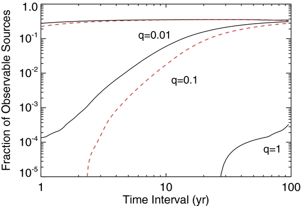
Figure 9. Fraction of observable SMBH binaries in next-generation surveys assuming that all SMBH binaries stall at sub-parsec scales forever due to depletion of stars with no subsequent evolution. The three pairs of lines correspond to mass ratio q = 1, 0.1, and 0.01 from bottom to top, respectively. The black solid lines utilize BH masses from broad-line width measurements, while the red dashed lines use the Eddington-limited BH masses estimated from bolometric luminosity. In the q = 1 case, the stalling radius (Equation (11)) is so large that no BH binaries are expected to be observed within 100 yr using the Eddington-limited BH mass distribution, so there is no red dashed line for it.
Download figure:
Standard image High-resolution image
The Subaru PFS (Takada et al. 2012), a new fiber-fed optical and near-infrared spectrograph that is now being planned, will be able to study QSOs over a wide redshift range. It will observe quasars down to i < 24 mag, which is much deeper than SDSS. It could also target up to 20 QSOs deg−2 from SDSS over the 1400 deg2 wide survey area. Therefore, nearly all the SDSS QSOs could be reobserved, providing a very large sample of QSOs with long-baseline repeat observations. Considering that the total quasar sample from DR7 is of order 105 objects, we can think of constraining binary fractions as low as ∼10−4, with time baselines greater than a decade, as potentially observable in the near future.
7. SUMMARY
We have employed a new method to search for sub-parsec SMBH binaries. We make use of repeat observations of quasars at 0.36 < z < 2 in the SDSS and look for temporal changes in the LOS velocity of the Mg ii broad emission line using cross-correlation. A radial velocity drift in the broad emission lines can be interpreted as an orbital acceleration of the accreting BH and its associated BLR. From the SDSS quasar catalog, we find a sample of 4204 quasars with multiple observations (1791 of them with Δt > 0.5 yr) and select 1523 quasars with S/N pixel−1 > 10 as a more reliable subsample. The absolute magnitude in g of the whole sample ranges from −18.4 to −27.5 mag with a mean value of −24.1 mag. We use two sets of BH masses: using Mg ii line widths, the BH masses range from 107–1010.5 M☉ and peak at 108.75 M☉; if we simply estimate a lower limit to the BH mass assuming that all sources radiate at 50% of their Eddington luminosity, we find a mass range of 106.3–109.8 M☉ and a peak at 108.3 M☉.
The velocity shifts measured by cross-correlation have a distribution peaked at 0 km s−1 with σ ∼ 100 km s−1 for the whole sample and σ ∼ 82 km s−1 for the high-S/N subsample. We set the following criteria for our SMBH binary candidates: the error in the cross-correlation should be <100 km s−1, the velocity shift measured with cross-correlation over either the whole spectral range or only the Mg ii line region should be larger than 3.4σ (280 km s−1), and the difference between the two measurements should be less than 1σ (∼82 km s−1). We select seven binary BH candidates out of the high-S/N subsample, of which three are most reliable. We are now following these up to search for continued evidence of orbital motion.
Comparing the detectability of SMBH binaries with the number of candidates (N ⩽ 7), we can rule out that all 109 M☉ BHs exist in ∼0.03–0.2 pc scale binaries, in a scenario where binaries stall at a sub-parsec scale radius for a Hubble time. In the scenario of gas-assisted SMBH binary evolution, our analysis reports that ≲16% of quasars host SMBH binaries with orbital separations <0.1 pc at their centers, subject to outstanding uncertainties in the BH masses and BLR sizes.
We should also ask what the cosmological expectations are for such binaries. While a full exploration is beyond the scope of this work, we note from the simulations of Volonteri et al. (2003) that massive host galaxies will have experienced numerous major ( ) mergers since redshift z ≈ 2. Furthermore, according to simulations, pairing of SMBHs via dynamical friction is most effective for major mergers (e.g., Callegari et al. 2009). Thus, our results are already cosmologically relevant. In the future, we may hope to constrain the lifetime of sub-parsec binaries with larger samples.
We also estimate the observability of SMBH binaries with next-generation surveys, such as BOSS or the PFS on Subaru, in the context of the disk-assisted inspiral scenario. With the reobservation of SDSS quasars by these new surveys, we will have a much larger sample with much longer time baselines to investigate the temporal change of broad emission lines. These future observations will help constrain evolutionary scenarios of SMBH binaries.
We thank an anonymous referee for substantially motivating us to improve this work. We thank Michael Strauss for helpful directions on SDSS data and inspiring discussions. We are also grateful for helpful comments from Bence Kocsis, Craig Loomis, Frans Pretorius, Alberto Sesana, Yue Shen, Sean McWilliams, Sarah Burke Spolaor, and Justin Ellis. Wenhua Ju thanks Petchara Pattarakijwanich for useful and patient discussions on IDL coding.
Footnotes
- 4
Definitions of Md different by factors of 2π or 4π can be found in the literature.