


ABSTRACT
High-resolution observations of the Sun's corona in extreme ultraviolet and soft X-rays have revealed a new world of complexity in the sheet-like structures connecting coronal mass ejections (CMEs) to the post-eruption flare arcades. This article presents initial findings from an exploration of dynamic flows in two flares observed with Hinode/XRT and SDO/AIA. The flows are observed in the hot (≳ 10 MK) plasma above the post-eruption arcades and measured with local correlation tracking. The observations demonstrate significant shears in velocity, giving the appearance of vortices and stagnations. Plasma diagnostics indicate that the plasma β exceeds unity in at least one of the studied events, suggesting that the coronal magnetic fields may be significantly affected by the turbulent flows. Although reconnection models of eruptive flares tend to predict a macroscopic current sheet in the region between the CME and the flare arcade, it is not yet clear whether the observed sheet-like structures are identifiable as the current sheets or "thermal halos" surrounding the current sheets. Regardless, the relationship between the turbulent motions and the embedded magnetic field is likely to be complicated, involving dynamic fluid processes that produce small length scales in the current sheet. Such processes may be crucial for triggering, accelerating, and/or prolonging reconnection in the corona.
Export citation and abstract BibTeX RIS
1. INTRODUCTION
In the rearrangement of magnetic fields that accompanies a coronal mass ejection (CME) and powers the energy release for a solar flare, current sheets are vital topological structures. The current sheet is critical as the location of magnetic flux transfer via magnetic reconnection, separating unreconnected flux streaming into the dissipation region from post-reconnection flux retracting away from the flux transfer site. The geometric structure of the current sheet is intimately linked to the rate of flux transfer: a thinner diffusion region allows faster transfer of the magnetic flux, and therefore a significantly greater reconnection rate. The rate of flux transfer is also dependent on the ease with which the magnetic flux can diffuse through the plasma, which in turn is affected by highly localized variations in the resistivity and viscosity of the plasma.
Sheet-like structures in post-CME solar flares have been observed in a wide range of wavelengths (white light, Ko et al. 2003; UV, Lin et al. 2005, 2007; Aurass et al. 2009; EUV, Innes et al. 2003; Reeves & Golub 2011; Warren et al. 2011; and X-rays, Gallagher et al. 2002; Savage et al. 2010; Savage & McKenzie 2011) for a large and growing number of CME-flare events. A recent example observed by SDO/AIA is shown in Figure 1. Starting with Švestka et al. (1998), the X-ray-emitting plasma between the closed-field arcade and the CME has been referred to as a "fan of coronal rays" (see also McKenzie & Hudson 1999; Khan et al. 2007; Savage & McKenzie 2011). Analyses of SOHO/UVCS and SOHO/LASCO data have tended to refer to the observed structure simply as the current sheet, identifying the entire feature with the topological boundary structure (Ciaravella & Raymond 2008; Lin et al. 2007; Webb et al. 2003; Ko et al. 2003). Savage et al. (2010) also made this identification in describing reconnection outflows observed in a current sheet-aligned feature detected in soft X-rays and EUV. It is natural to associate the fan with a current sheet linking the CME to the flare arcade, owing to its location, shape, and timing/persistence of appearance. However, the current sheet is expected to be far thinner than can be resolved with present-day observing instruments—on the order of a few tens of meters (Wood & Neukirch 2005 and references therein). Although some effort has been made to reconcile this expectation with the observations (e.g., via turbulent broadening of the current sheet; Bemporad 2008), it is still unclear whether the observed structure is the current sheet or a sheath of hot plasma surrounding the current sheet. Seaton & Forbes (2009), in discussing their model of plasma heating via conduction along field lines out of the current sheet, referred to this sheath as a "thermal halo." While it seems likely that the features observed in UV, EUV, and X-rays are due to emission from such a thermal halo, we cannot observationally distinguish the current sheet from the thermal halo. Therefore, in the following we shall refer to the structure as the "current sheet/thermal halo," or CSTH. These extended features are taken as evidence of macroscopic current sheets wherein magnetic reconnection takes place. While numerical models are beginning to reproduce the temperatures and general, two-dimensional appearances in EUV and X-rays (Reeves et al. 2010; Ko et al. 2010), it is the local conditions within this region that are key for controlling the magnetic reconnection.
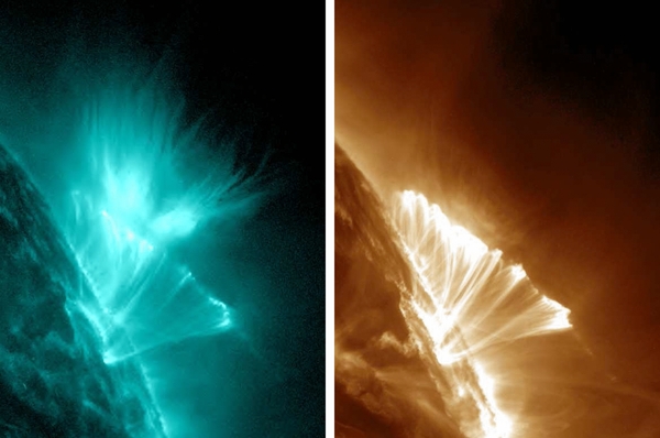
Figure 1. SDO/AIA images from 2011 October 22. In the left-hand panel, the arcade and current sheet/thermal halo appear in 131 Å radiation at 13:23:45 UT. In the right-hand panel, a nearly simultaneous image (13:23:55 UT) in 193 Å reveals the arcade and very faint emission from the supra-arcade region, consistent with a temperature of the current sheet/thermal halo ≳ 10 MK.
Download figure:
Standard image High-resolution imageOnly recently have high-resolution observations become possible with the capability to scrutinize the conditions within the sheet area. The most recent data from space-based telescopes reveal an environment far more complex than the simple laminar current sheets envisioned in two-dimensional and 2.5-dimensional models of reconnection. In this article, findings from an exploration of the velocity fields in the supra-arcade current sheet/thermal halo, as imaged by SDO/AIA (Pesnell et al. 2012; Lemen et al. 2012) and Hinode/XRT (Kosugi et al. 2007; Golub et al. 2007; Kano et al. 2007), will be presented. To track the changing location of emitting plasma, interpreted as flows within the CSTH, a local correlation tracking method is applied to the XRT and AIA image sequences of the CSTH in two flares. The results of the local correlation tracking reveal strong velocity shears and apparent vortical/rotational motions. An argument is made, based on temperature and density estimates, that the plasma β (the ratio of gas pressure to magnetic pressure) in at least one of the CSTH is of the order of unity. In such a (comparatively) high-β regime, turbulent flows may significantly contort the embedded magnetic field, and steep gradients in velocity provide conditions for fluid instabilities, which may contribute to the reduction of spatial scales in the current sheet/thermal halo. Such processes may be crucial for triggering, accelerating, and/or prolonging reconnection.
2. MEASUREMENTS
The occurrence of CSTH structures is well documented in a large number of eruptive solar flares; see Savage & McKenzie (2011) for an extensive yet inexhaustive listing of observations in EUV and soft X-rays. Two flares were selected, and local correlation tracking, a technique most often applied in deriving photospheric velocity fields (November & Simon 1988; Chae 2001), was applied to high-resolution image sequences of the CSTH. The figures below show the results of applying the Fourier local correlation tracking technique (FLCT; Fisher & Welsch 2008) to SDO/AIA images of the 2011 October 22 CSTH, the same event depicted in Figure 1, and to Hinode/XRT images of a limb flare of 2007 May 8. Readily apparent are strong velocity shears, converging/stagnating flows, and transient vortices. The velocities calculated with FLCT are verified by advecting simulated test particles ("corks") and overplotting the corks on the original AIA/XRT movies for comparison. Finally, an estimate of the vorticity was calculated by finding the curl of the FLCT velocities.
2.1. 2007 May 8, Hinode/XRT
On 2007 May 8, a flare occurred on the west limb of the Sun in association with a minor CME. The X-ray flux from the flare reached a level of only B1.2 on the GOES scale, due to the location beyond the limb; the Solar Object Locator (Sol. Phys. Ed. 2010) is SOL2007-05-08T10:07:00L308C101. Hinode/XRT observed the event with full (1.03 arcsec pixel−1) resolution and a 512×512 (pixels) field of view. The XRT observing program produced a movie in the titanium-on-polyimide (Ti-poly) filter with a 30 s cadence, alternating every 20–30 minutes with a lower cadence set of images in multiple filters. The analysis herein focuses on a 20-minute-long sequence of Ti-poly images (i.e., 40 images with a 30 s cadence) from 10:33:08 UT to 10:52:38 UT. The data were prepared using the standard xrt_prep utility in SolarSoft (Freeland & Handy 1998). The Hinode spacecraft pointing was very stable over this time interval, so no special steps were taken to improve co-alignment of the 40 images. An extracted portion of the field of view, showing the southern part of the flare CSTH, is shown in Figure 2.
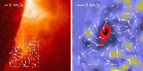
Figure 2. Coronal vortex observed with XRT, 2007 May 8. The background image of the left-hand panel shows the location of the flaring active region on the west limb. The colored background of the right-hand panel demonstrates the vorticity calculated from the curl of the velocity field. In both panels, the FLCT-derived velocity field is overplotted as arrows. The white bar at upper left in each frame represents a velocity magnitude of 5 km s−1, for scale.
Download figure:
Standard image High-resolution imageAlthough some dynamic activity is seen in other parts of this eruptive structure, the most notable feature in this 20-minute interval is apparent rotation in the southernmost part of the extended coronal structure, immediately above the limb. The rotation appears to persist throughout the 20-minute span of the selected data, and so for the present study a 100 × 100 pixel region centered on that rotation was isolated for analysis. To enhance the sensitivity of the FLCT to motions of the more faintly emitting plasma, a logarithmic dynamic range compression was applied (i.e., the log10 of the XRT signal was analyzed). The chosen 100 × 100 (pixels) region is indicated by velocity arrows shown in Figure 2.
A detailed description of the FLCT algorithm, including the use of a signal threshold (below which the image intensity is ignored) and the width of sub-regions to be cross-correlated, is given in Fisher & Welsch (2008). Experimentation with the FLCT applied to the extracted XRT data led to the selection of a signal threshold of t = 0.45 DN s−1 pixel−1, and Gaussian width σ = 8 pixels as yielding the best combination of sensitivity, repeatability, and low rate of spurious velocity field structures. The FLCT was applied to all 39 pairs of adjacent (in time) images, yielding 39 sets of vx, vy arrays. The vx velocities correspond to motions east–west, while vy represents motions north–south; vz, normal to the plane of the sky, was assumed to be zero. To assist in the selection of the FLCT parameters, an advection code was developed to verify the fidelity with which the FLCT-derived velocities represented the motions in the CSTH: several hundred test particles (virtual "corks") were arrayed across the 100 × 100 region of interest and then advected through the 39 time steps via application of the 39 velocity snapshots. The corks advected in this way were overplotted on the XRT images as a way to check that their motions matched the flows in the CSTH.
In order to visualize the 20-minute-long rotational trend, while reducing the noise in the velocity measurements, the 39 vx, vy pairs were averaged in time to yield a single vx, vy pair (i.e., [100 × 100 × 39] reduced to [100 × 100]). The arrows in Figure 2 show the averaged velocities at every 10th pixel within the 100 × 100 region of interest. While most of the averaged velocities were smaller than 70 km s−1, a handful were greater than 100 km s−1; the median averaged speed is 3.6 km s−1 and the median absolute deviation is 2.1 km s−1. The vorticity (plotted in Figure 2) was found by first calculating the curl from each of the 39 vx, vy array pairs. Each of the 39 curl images was then smoothed via boxcar median smoothing to reduce noise and summed together to yield a single 100 × 100 array of vorticity over the full 20-minute span. Measurement of the magnitude of the vorticity is very noisy in the absence of smoothing: in the core of the vortex (dark red to black in Figure 2) the peak magnitude in the 39 snapshots before smoothing is generally between 2 km s−1 pixel−1 and 20 km s−1 pixel−1 (into the plane of the sky), with a few excursions to 40 km s−1 pixel−1 and beyond. After boxcar median smoothing, the peak vorticity in the same region is consistently 1–3 km s−1 pixel−1. Averaged over the 39 time steps, the peak (median) vorticity in the core is 0.8 (0.6) km s−1 pixel−1.
2.2. 2011 October 22, SDO/AIA
On 2011 October 22, a GOES M1.3 flare was observed with multiple instruments on the northwest limb of the Sun in NOAA active region number 11314. The flare began at 10:00 UT and reached its peak in soft X-rays more than an hour later, at 11:10 UT; this event (SOL2011-10-22T10:00:00L045C065) has previously been described by Savage et al. (2012) and is associated with a major CME. The event was observed by SDO/AIA, which made images with angular resolution 0.6 arcsec pixel−1 and observing cadence of one image per 12 s in each of its several wavelength channels. The CSTH is detectable in AIA's 131, 94, and 193 Å channels; however, the analysis herein uses only the 131 Å data because (for this event) the visibility of the CSTH is best and most extensive in that channel (Figure 1). The data were downloaded from the AIA cutout service provided by the Lockheed Martin Solar and Astrophysical Laboratory1, and thus were pre-calibrated for instrumental effects, with a spatial filtering applied to select the flare region of interest. The data were downselected to 75 images between 11:48:09 UT and 12:47:21 UT, with an effective cadence of one image per 48 s.
In order to emphasize the motions and changes in the CSTH during the selected interval, a mean image was calculated, and each of the 75 images was divided by that mean. Noise reduction was accomplished by boxcar median smoothing. Finally, the region of interest including the CSTH above the arcade was selected for analysis. The resulting enhanced movie, clearly showing the complexity of the velocity field, accompanies the article in the online journal. One snapshot from the enhanced movie is shown in Figure 3.

Figure 3. FLCT analysis of the 2011 October 22 CSTH, 12:32:09 UT snapshot. The upper left panel shows the appearance of the flare arcade and CSTH in log10 of the 131 Å intensity. The upper right panel shows the CSTH region after enhancement as described in the text. The whole CSTH area was analyzed with FLCT, but for clarity only the streamlines in the white box are shown in the bottom left panel. Velocity shears are implied by high speeds next to low speeds, or oppositely directed arrows. A stagnation appears near top center, as well as a vortex in upper right. The bottom right panel is a snapshot of vorticity, calculated as described in the text. Movies of the two right-hand panels accompany the online article.(Animations (3a and 3b) of this figure are available in the online journal.)
Download figure:
Standard image High-resolution image
The FLCT was applied to each of the 74 image pairs, with signal threshold t = 0.25 DN s−1 pixel−1 and Gaussian width σ = 18 pixels. Just as for the 2007 May 8 event, the velocities were checked via several hundred virtual corks advected across the region of interest by application of the 74 velocity snapshots. The corks advected in this way were overplotted on the AIA images to check that their motions accurately represented the flows in the CSTH. Speeds up to 250–300 km s−1 were found to occur consistently throughout the hour-long sequence. Discounting outliers in excess of 350 km s−1, the median speed found in the CSTH is 38 km s−1 and median absolute deviation is 30 km s−1.
In contrast to the XRT sequence analyzed above, where only one vortex was apparent, in the AIA sequence far more action is visible. Streamlines plotted from the FLCT velocities reveal numerous velocity shears, apparent stagnations, and temporally varying vorticities (e.g., Figure 3). Rather than time-averaging the full duration of velocities and summing the vorticity, a movie of vorticities was prepared: after calculating the vx, vy snapshots for 74 image pairs, the curl was calculated for each, yielding 74 snapshot maps of vorticity. The noise was reduced via boxcar median smoothing and the running mean of vorticity displayed in the movie accompanying the online version of this article, one frame of which is shown in Figure 3. This may be the first movie of its type, recording vorticities in the solar corona, observed in EUV. The movie reveals a series of small pockets of vorticity (i.e., vortices) moving downward toward the flare arcade. Frequently pairs of positive and negative vortices move together: these pairs appear at the locations of the supra-arcade downflows reported by Savage et al. (2012). The magnitude of the velocity curl (i.e., the vorticity) in the moving vortices is measured to range between −1.4 km s−1 pixel−1 and +1.6 km s−1 pixel−1. These measurements were made primarily from the more intense vortices, those that are most visible in the movie. The least intense vortices examined had magnitudes of ≈0.4 km s−1 pixel−1. These values should only be interpreted as an estimate of the magnitude of the more intense vortices, and not the full range nor the lower limit of detectability.
3. DISCUSSION
As noted above, the curl of the FLCT velocity field yields an estimate of vorticity. The FLCT velocities considered herein are necessarily in the plane of the sky, due to the nature of the observations. While motions along the line of sight (LOS) may be significant, the present data set offers no straightforward way to address them. In the absence of spectroscopic measurements, we are left to speculate on the degree to which the flows out of the image plane—and transverse to the unreconnected magnetic field surrounding the current sheet—are contained by the inflow of plasma and magnetic field to the current sheet. It is noteworthy, however, that the median FLCT velocity found in the 2011 October 22 event is of the same order as turbulent speeds inferred from nonthermal broadening in spectroscopic flare measurements (e.g., Antonucci et al. 1996; Ciaravella & Raymond 2008; Milligan 2011 and references therein).
It is unknown at this time whether the vorticity of the order of 1 km s−1 pixel−1 estimated from the XRT sequence corresponds to the uncoiling of a twisted flux rope, or (perhaps less likely) the coiling up of a flux rope. The arrows in Figure 2 do not appear to resemble a simple shear of sunward and antisunward flows side by side.
The complex flows described above, especially flows of the type seen in the 2011 October 22 event, are likely to be crucial for creating the small lengthscales required for fast reconnection (cf. Lapenta & Lazarian 2012 who find "magnetic reconnection in the presence of turbulence is always fast"). For example, signatures of Kelvin–Helmholtz instabilities (KHIs) have been detected previously in a CME-related flare (Ofman & Thompson 2011). Soler et al. (2012) indicate that KHIs can be triggered by shearing flows in the presence of plasma viscosity and contrasting densities along interfaces. The FLCT results for the 2011 October 22 event clearly show velocity shears, and the AIA images and differential emission measure (DEM) maps (Savage et al. 2012) reveal density gradients. The conditions would appear to be favorable for KHIs, though signatures of the instability have not been unambiguously detected in the CSTH.
A comparison may be made to the upflows and plumes in prominences detected by Hinode/SOT (Berger et al. 2008, 2010) and also seen in observations from Mauna Loa (de Toma et al. 2008); although in the prominences buoyancy appears to play a more significant role than seems likely in the CSTH, given that the flows in the CSTH are sunward. The model by van Ballegooijen & Cranmer (2010) implies a high degree of field line tangling in prominences subjected to such complex flows. It is perhaps reasonable to expect similar tangling in the CSTH, producing a stochastic magnetic field and micro-current sheets as envisioned by Lazarian & Vishniac (1999).
An interpretation of the CSTH observations in terms of plasma turbulence distorting the embedded magnetic field implies plasma β that is closer to unity than is commonly expected in the solar corona. Gary (2001) demonstrates that plasma β, the ratio of gas to magnetic pressure, is on order of 10−2 for much of the corona; but also shows that for heights above 50 Mm, β > 0.1 may be widespread, and above 100 Mm one might expect β values in excess of 0.5. Quantitative analysis of the image data tends to bear out such an expectation. Considering specifically the 2011 October 22 event, a useful estimate of the plasma temperature is provided by DEM analysis. The DEM map displayed by Savage et al. (2012) indicates the most prevalent temperatures in the CSTH are 8–13 MK; this DEM was subsequently revised by K. Reeves (2012, private communication) to show that temperatures 13–20 MK are significantly more common. With the DEM as a guide, and with the understanding that conditions in the CSTH are likely to vary both spatially and temporally, a temperature of 13 MK is assigned to this CSTH for the purpose of estimating β. This temperature is consistent with the faint visibility of the CSTH in 193 Å, due to Fe xxiv (Figure 1), and numerous previous observations of CSTH in Fe xxi and Fe xxiv (Innes et al. 2003; Verwichte et al. 2005, e.g.). The same DEM analysis indicates a column emission measure in the middle-to-lower parts of the CSTH near 5 × 1027 cm−5; higher up, the emission is only slightly lower, ≈2 × 1027 cm−5. The LOS depth is difficult to measure, as the available STEREO-A/EUVI images of the event (see Savage et al. 2012, their Figure 2) do not clearly show the CSTH. However, the analysis by Savage et al. (2010) of an earlier, similar event indicates an upper limit on the thickness in soft X-rays of approximately 4–5 Mm, indicating an electron density in the CSTH of at least 3 × 109 cm−3 at the bottom of the CSTH (≈0.15 R☉ above the photosphere), and 2 × 109 cm−3 at a height of 0.25 R☉. (The LOS depth is a conservative estimate, due to the resolution of Hinode/XRT images, and possibly projection effects as noted by Savage et al. (2010). The true depth may be smaller, which would suggest higher density and higher β.)
The magnetic field strength in the supra-arcade region is estimated from the potential field source surface extrapolation provided by M. DeRosa and C. Schrijver (i.e., pfss_viewer) in SolarSoft. The extrapolated field for 2011 October 22, 06:00 UT (i.e., before the flare) was selected, and then the Br, Bθ, and Bϕ components were added in quadrature for heights 0.15 R☉–0.25 R☉ above the photosphere. This yielded |B| between 4 and 11 G, decreasing with height. An independent magnetic charge topology extrapolation by D. Longcope (2012, private communication) found |B| of 4–12 G for the same region. Since the true magnetic field strength in this flaring region is likely to be higher than these potential-field extrapolations suggest, the plasma β was calculated after amplifying the extrapolated |B| to 6–16 G. (Again, this is a conservative estimate. Omission of the semi-arbitrary 50% amplification yields higher values of β.)
Thus with T = 13 MK, ne = 2–3× 109 cm−3, and |B| = 6–16 G, the plasma β is estimated according to
indicating β ≈ 1.1 near the base of the CSTH, and β ≈ 5 higher up. Rather than the CSTH plasma being magnetically dominated, one should consider that significant interplay between magnetic and gas-pressure forces is present throughout the CSTH.
One may also question whether the plasma can reasonably be considered to behave as a fluid. After all, with density 3 × 109 cm−3 and temperature 13 MK, a nominal estimate of proton (electron) mean free path would be 5 (3) Mm, comparable to the size of the structures seen in the images. Because of the presence of the magnetic field, however, the relevant size to consider is not the (unmagnetized) mean free path, but the ion gyroradius. Given the conditions described above, the proton gyroradius in the CSTH is of the order of 2–6 m. With scale sizes in the coronal images on the order of megameters, the Knudsen number in the CSTH is far smaller than unity, suggesting that treatment as a fluid continuum is appropriate.
The number of particles contained in a sphere of radius equal to the Debye length, ND, gives an alternative measure of the appropriateness of a fluid treatment. If the plasma parameter gp ≡ ND−1 is much smaller than unity, then the particles are numerous enough for the system to be treated as a fluid. Given T = 13 MK and ne = 3 × 109 cm−3, the Debye length can be expressed as λD = 7.0(T/ne)1/2 = 0.46 cm, and
so that gp = 8 × 10⁻¹⁰ ≪ 1.
The size of the smallest eddies, the scale on which viscous dissipation converts kinetic energy into heat, is determined by the magnitude of the plasma viscosity. Numerous authors have commented on the importance of viscous heating in the flare energy budget—perhaps even surpassing Joule heating (Hollweg 1986; Craig 2010)—and as a factor in stabilizing the magnetic system against MHD instabilities (Shan & Montgomery 1993). However, the viscosity in a magnetized plasma is highly anisotropic, with components parallel and perpendicular to the magnetic field differing by several orders of magnitude. The presence of turbulence in a high-β regime complicates any study of viscous effects much further, as the magnetic field strength and direction, as well as the plasma density and pressure, become extremely variable on a wide range of temporal and spatial scales. Such a study of viscous effects is beyond the scope of the present article.
However, further observational investigations of the turbulent velocity fields in CSTH are likely to be useful in guiding efforts to model post-CME current sheets, particularly in regard to cascades from CME length scales to much smaller sizes, and the contortions to embedded magnetic fields that result. For example, Dmitruk et al. (2004) employed a model of turbulent MHD to deform an input magnetic field and then held the distorted field constant while test particles were accelerated from rest in the post-turbulence field. They found that electrons and protons responded very differently to the conditions in the distorted field. One can imagine using the FLCT results from post-CME CSTH to deform an assumed initial field, in a continuous way (as opposed to freezing the field as in Dmitruk et al. 2004), and determining the forces on electrons and ions in/near the current sheet. Bárta et al. (2009) introduce a framework for modeling the wide range of scales that are present in current sheet reconnection and demonstrate the feasibility of simultaneously modeling multiple scales; the authors were able to reproduce secondary magnetic islands/plasmoids in a two-dimensional current sheet and suggest that the technique could be used to explore a fractal current sheet of the sort envisioned by Shibata & Tanuma (2001). High-resolution observations such as those presented herein help to ascertain the length scales that are present in the CSTH, and may help to shape the development of these models. Bemporad (2008) estimates upper limits of the turbulent velocities in CSTH from Ultraviolet Coronagraph Spectrometer (UVCS) data and uses those observations to derive estimates of turbulent energy density, anomalous resistivity, and the size and number density of micro-current sheets. It is reasonable to presume that these values can be refined with higher resolution, time-resolved observations of turbulence in the CSTH.
The length and velocity scales inferred from the images and the FLCT can be used to place limits on such transport coefficients as the eddy magnetic diffusivity (Priest 1982, p80). Taking v ≈ 38 km s−1 (median from the 2011 October 22 event) and d ≈ 2 × 108 cm (typical size of the smallest identifiable vortices in the same event) and following Priest's formulation, the eddy magnetic diffusivity is found to be  cm2 s−1. This
  is significantly larger than those listed by Priest (1982) for the photosphere. However, this should be considered an upper limit, until more reliable estimates of the sizes of the smallest eddies in the CSTH can be obtained with high-resolution imaging and/or spectroscopy. The inferred
  is also much larger than the diffusion coefficients estimated from motions of features in high-resolution magnetographs in more recent studies, although it should be noted those diffusion coefficients are defined differently than
  . See especially the excellent summary by Abramenko et al. (2011). The difference in diffusivity estimates between this study and the photospheric scales should not be taken as direct evidence for super-diffusion—i.e., diffusion coefficient growing with spatial and temporal scale (again, see Abramenko et al. 2011 for a review)—until more reliable measurements in CSTH can be made with higher spatial resolution.
4. CONCLUSIONS
The investigation described herein explores the extremely dynamic motions observed in sheet-like structures above post-CME flare arcades and highlights the advantage of high-resolution observations in the corona. Recent developments in EUV and X-ray imaging provide the combination of high spatial and temporal resolution, and sensitivity to emissions from plasmas with temperatures >10 MK, that make it possible for the first time to image and characterize the turbulence in the region associated with the current sheet. Local correlation tracking facilitates the characterization of flows and calculation of parameters in the velocity field. The flows are extremely complex and variable, including variable velocity shears, convergences/stagnations, and vortices. The plasma β is found to be of the order of unity in at least one of the flares studied and is expected to behave similarly in other CSTH. These findings demonstrate that turbulent effects are present in or very near the current sheets in CME-associated eruptive flares. This turbulence very likely has significant effects on the magnetic field, and possibly on the current sheets, including contortions to the magnetic field (and the possibility of stochastic fields), and cascades to small length scales. The resulting conditions are likely to have profound effects on the rate of magnetic reconnection. Further observational characterization of the turbulent conditions will help to guide efforts in modeling post-CME current sheets, particularly in regard to cascades from CME length scales to much smaller sizes.
Exploration of the turbulent conditions in the flaring solar corona is the realm of high-resolution, high-cadence imaging and spectroscopy in the corona, such as is now possible with Hinode/XRT, Hinode/EIS, and SDO/AIA. Further investigation with these and future higher resolution coronal imagers and spectrographs promises to enable fuller characterization of the spectrum of velocities and vorticities, the range of eddy sizes, and the frequency of instabilities like KHIs.
This work was supported by NASA under contract SP02H3901R from Lockheed-Martin to Montana State University, and contract NNM07AB07C with the Smithsonian Astrophysical Observatory. The author wishes to thank the anonymous referee for very useful suggestions.