


ABSTRACT
We present a new three-dimensional numerical method for calculating the non-spherical shape and internal structure of a model of a rapidly rotating gaseous body with a polytropic index of unity. The calculation is based on a finite-element method and accounts for the full effects of rotation. After validating the numerical approach against the asymptotic solution of Chandrasekhar that is valid only for a slowly rotating gaseous body, we apply it to models of Jupiter and a rapidly rotating, highly flattened star (α Eridani). In the case of Jupiter, the two-dimensional distributions of density and pressure are determined via a hybrid inverse approach by adjusting an a priori unknown coefficient in the equation of state until the model shape matches the observed shape of Jupiter. After obtaining the two-dimensional distribution of density, we then compute the zonal gravity coefficients and the total mass from the non-spherical model that takes full account of rotation-induced shape change. Our non-spherical model with a polytropic index of unity is able to produce the known mass of Jupiter with about 4% accuracy and the zonal gravitational coefficient J2 of Jupiter with better than 2% accuracy, a reasonable result considering that there is only one parameter in the model. For α Eridani, we calculate its rotationally distorted shape and internal structure based on the observationally deduced rotation rate and size of the star by using a similar hybrid inverse approach. Our model of the star closely approximates the observed flattening.
Export citation and abstract BibTeX RIS
1. INTRODUCTION
As a consequence of rapid rotation, planets like Jupiter are rotationally distorted into a non-spherical shape. Taking the full effect of rotational distortion as the leading-order solution in describing the shape and gravity of a rotating gaseous planet leads to a highly complicated and challenging mathematical problem. Although attempts to employ spheroidal geometry as the leading-order solution have been made with constant density (Kong et al. 2012; Hubbard 2012), the generalization of the constant density models to compressible gaseous models, via either analytical or semi-analytical approaches, is likely too complicated to be practical. No previous attempts have been made to compute the gravitational field of a rapidly rotating, compressible fluid planet that accounts for the full effects of rotation.
This paper represents the first attempt to calculate a model of the gravitational field of a rapidly rotating compressible fluid body when the rotational distortion is too large to be regarded as a small perturbation. In such a calculation, an equation of state (EOS) describing the relationship between the pressure p and the density ρ, denoted by p = f(ρ), is needed. There are at least three different types of EOS that may be adopted: a physical EOS (Chabrier et al. 1992; Saumon et al. 2004; Nettelmann et al. 2012), an empirical EOS (Helled et al. 2009), and the classic polytropic EOS (Chandrasekhar 1933, 1967; Hubbard 1974, 1999). In this study, we adopt the EOS of a polytrope of index unity for the following reasons. First, a polytrope of index unity has been shown to provide a good qualitative approximation to the EOS of the Jovian interior (Hubbard 1974, 1999). Second, a simple polytropic EOS is appropriate for illustrating our method of studying rotationally distorted bodies without making any approximation, which is the primary focus of this paper. Third, the existence of the analytical solution of Chandrasekhar (1933) for the polytropic EOS allows us to validate our numerical results. Finally, the proposed method for the simple polytropic EOS can be readily extended to other more realistic EOS without any major mathematical or numerical difficulties.
We present a new numerical model, based on a finite-element method, for determining the rotationally distorted shape and internal structure of a rapidly rotating gaseous body whose EOS is that of a polytrope of index unity; in the EOS for a polytrope,

where n is the polytropic index and K is a constant, we take n = 1. A significant consequence of choosing n = 1 is that the resulting governing equation of the equilibrium state for the density ρ is linear.
The internal structures of slowly rotating planets and stars with a polytropic index of unity n = 1 was first studied by Chandrasekhar (1933) using a perturbation analysis. For an isolated, non-rotating, and self-gravitating body, the density distribution ρ0 within its interior is spherically symmetric and described by the Lane–Emden equation
where r is the radial coordinate in spherical polar coordinates and G is the universal gravitational constant with G = 6.67384 × 10⁻¹¹ m3 kg−1 s−2. With a proper boundary condition for ρ0, the Lane–Emden equation can be readily solved to determine the one-dimensional density distribution of such non-rotating masses. For a body that is slowly rotating with angular velocity Ω0 such that departure from spherical symmetry is small, Chandrasekhar (1933) introduced a small parameter  ∼ Ω2
0 and, then, wrote the density distribution ρ in a perturbation series
∼ Ω2
0 and, then, wrote the density distribution ρ in a perturbation series

He solved the first-order solution Ψ by neglecting the effects arising from the second-order term Φ. Martin (1970) extended the first-order solution of Chandrasekhar (1933) to the second order by obtaining Φ in the expansion (3).
Many gaseous bodies such as Jupiter and Saturn are rotating rapidly and thus cause significant departure from spherical geometry: the eccentricity at the one-bar surface is  for Jupiter and
  for Saturn (Seidelmann et al. 2007). Classical perturbation theories (Chandrasekhar 1933; Hubbard 1974; Zharkov & Trubitsyn 1978) based on an expansion around spherical geometry using a small rotation parameter require an unpractically large number of terms in the expansion to reach the high precision anticipated in Juno's observations of Jupiter's gravitational field (Kaspi et al. 2010). Some stars, such as α Eridani (Domiciano de Souza et al. 2003), rotate even faster and result in an even larger departure from spherical geometry. It is thus highly desirable, in order to provide an accurate description of the structure and gravity for these rapidly rotating bodies, to construct a non-spherical model that takes full account of rotational distortion.
This paper examines the shapes and internal structures of rapidly rotating gaseous bodies having a polytropic interior with an index of unity and the shape of an oblate spheroid of moderate or large eccentricity. The governing equations of the problem are solved using a three-dimensional finite-element method by making a three-dimensional tetrahedralization of the oblate spheroid that produces a finite-element mesh without pole or central numerical singularities. Though a finite-element model is usually complicated and cumbersome in its numerical implementation, it is particularly suitable for non-spherical geometry for which the standard spectral method would be mathematically inconvenient and difficult. In comparison with an analytical approach (Chandrasekhar 1933), there are, however, two major difficulties in numerical modeling. Prior to solving the equations for the shape of a rapidly rotating body, we must construct a three-dimensional finite-element mesh on which we can compute a numerical solution to the equilibrium equations. The finite-element mesh is, however, dependent on the priori unknown shape of the rotating body. This difficulty will be resolved using an iterative procedure, which is numerically expensive, between the unknown shape (the finite-element mesh) and the required boundary condition by introducing an auxiliary function, in connection with the total potential, evaluated at the bounding surface of the rotating body. Another difficulty concerns the value of K in the EOS (1) which is also a priori unknown. When the polytropic index is fixed with n = 1, the value of K in the EOS also depends on the shape of the rotating body. We will utilize the observed shape of a rapidly rotating planet to determine the value of K by introducing a second iterative procedure. Meanwhile, a simple theoretical approach, presented in the Appendix, is also employed to estimate the value of K for gaseous planets.
In what follows we begin by presenting the governing equations and the numerical method in Section 2. The validation of our numerical model with the first-order asymptotic solution of Chandrasekhar (1933) is discussed in Section 3. We then apply the numerical model to Jupiter and α Eridani in Section 4. A summary and some remarks are given in Section 5.
2. GOVERNING EQUATIONS AND NUMERICAL METHOD
2.1. Governing Equations
Consider an isolated mass of gas with total mass M that is rotating rapidly about the z-axis with angular velocity  . When the density ρ = ρ0 is uniform, i.e., ρ0 is constant, the rotating fluid body is in the shape of an axisymmetric oblate spheroid with eccentricity
  given by the well-known equation (Lamb 1932):
When the density ρ within a rapidly rotating body is non-uniform, it was shown analytically that the leading-order solution is also in the shape of an axisymmetric oblate spheroid (Kong et al. 2010). In this study, we assume that the effect of rotation is sufficiently strong that the rotating body is in the shape of an oblate spheroid with moderate or large eccentricity that is still within the stable limit.
With a polytrope of index unity, the pressure–density relation of the gas is given by

where K is a constant. The mechanical equilibrium equation is
where Vg
is the gravitational potential, Vc
is the centrifugal potential, and  is the domain of the rotating body, subject to the boundary condition

The shape of a rotationally distorted body is characterized by its eccentricity  defined as
where  and, Re
and Rp
are the equatorial and polar radii of an oblate spheroid, respectively. In Equation (6), the gravitational potential Vg
is given by
and, Re
and Rp
are the equatorial and polar radii of an oblate spheroid, respectively. In Equation (6), the gravitational potential Vg
is given by
where  is the position vector. The centrifugal potential Vc
is
is the position vector. The centrifugal potential Vc
is
Here we have used oblate spheroidal coordinates, (ξ, η, ϕ), defined by the coordinate transformation with Cartesian coordinates
where c is the focal length of an oblate spheroid with its bounding surface  described by
The shape parameter, the size of eccentricity  , is a priori unknown.
On the bounding surface  of a rotating body, the free-surface condition must be imposed at the equilibrium

Eliminating p from Equations (5) and (6) yields the equation

which, after applying  to the both sides, becomes

After scaling Equation (12) with the length scale Re and the mass scale M, we obtain the governing equation in the dimensionless form

where α and β are defined as
The boundary condition (7), after using the EOS, becomes

Since α is always positive, Equation (13) represents an inhomogeneous Helmholtz equation (Chandrasekhar 1933). The condition of the free surface in Equation (10) can also be written in the dimensionless form
which must be satisfied at the equilibrium. Our primary task is to solve the inhomogeneous Helmholtz equation (13) for both the shape parameter  and the density distribution ρ(ξ, η) that satisfy both Equations (15) and (16).
When the shape parameter  and the density distribution ρ(ξ, η) become available for a highly flattened planet, we can readily compute the total mass of the rotating body
and the exterior gravitational potential Vg which is expanded in terms of spherical harmonics P2n ,
where (r, θ, ϕ) are spherical polar coordinates with θ = 0 being at the axis of rotation, and J2, J4, J6, ⋅⋅⋅, are the zonal gravitational coefficients. It is important to point out that Equation (18) is only valid for r ⩾ Re where there is no mass and the potential satisfies Laplace's equation. This is because the region Rp < r < Re has empty space in part and mass near low latitudes and, consequently, the potential satisfying Poisson's equation with the density is a highly complicated function of latitude and radius.
2.2. Numerical Method
A three-dimensional finite-element method is employed to solve the shape and internal structure of a non-spherical body through the following three different stages. The first stage is to construct a three-dimensional finite-element mesh by making a tetrahedralization of an oblate spheroid with a guessed eccentricity  . This is because we do not have a priori knowledge of the shape of a rapidly rotating liquid planet. A sketch of the finite-element mesh for an oblate spheroid with
  is illustrated in Figure 1(a). In comparison to a spectral or finite difference method, the finite-element method is free of the pole and central numerical singularities.

Figure 1. (a) Sketch of a three-dimensional tetrahedral mesh for an oblate spheroid with  and (b) the location of 10 nodes in a typical tetrahedral element.
Download figure:
Standard image High-resolution imageIn the second stage, we solve Equation (13) for ρ together with the boundary condition (15) with a given α and β for a guessed eccentricity  . A Galerkin-weighted residual approach is adopted in the finite-element formulation of Equation (13). Multiplying Equation (13) by the corresponding weight functions wρ, then integrating the resulting equation over the spheroidal domain
  , after making use of integration by parts, we derive the weak formulation of Equation (13)
where the boundary integral vanishes as the weight function wρ is zero on the bounding spheroidal surface  . Within each tetrahedron, as shown in Figure 1(b), 10 nodes are used in representing the density ρ
where ρj is the value of the density ρ on the jth node in the element and Φj is the quadratic function defined as
where Lj , j = 1, ⋅⋅⋅, 4 are the volume coordinates of the finite element and Φj has the properties
where  is the position vector for the ith node in the element. The weight functions are selected to be the same as the corresponding shape functions. Applying a standard procedure of the finite-element method, we obtain a system of linear equations for the coefficients ρj
on the whole three-dimensional mesh, which is then solved by a Krylov subspace iterative method. The values of ρj
on the mesh provide a numerical solution ρ(r) that satisfies Equations (13) and (15). For the results reported in this paper, a spheroidal domain is typically divided into about 106 ∼ 2 × 10⁶ tetrahedral elements.
is the position vector for the ith node in the element. The weight functions are selected to be the same as the corresponding shape functions. Applying a standard procedure of the finite-element method, we obtain a system of linear equations for the coefficients ρj
on the whole three-dimensional mesh, which is then solved by a Krylov subspace iterative method. The values of ρj
on the mesh provide a numerical solution ρ(r) that satisfies Equations (13) and (15). For the results reported in this paper, a spheroidal domain is typically divided into about 106 ∼ 2 × 10⁶ tetrahedral elements.
It is critically important to note that a numerical solution found in the second stage does not, in general, satisfy the free-surface condition (16). Although condition (16) is mathematically simple, it is numerically problematic. In order to find a numerical solution satisfying Equation (16), we introduce an auxiliary function, || dVt / dη||2, defined as
where  represents the surface integral over the bounding surface
  of the oblate spheroid. Theoretically, we would expect that
in the neighborhood of an equilibrium while
at the equilibrium. Far away from the equilibrium, we would have
Numerically, however, the mathematical condition || dVt /dη||2 = 0 cannot be exactly satisfied at the equilibrium. Instead, || dVt / dη||2 = 0 will be replaced by a numerical condition that || dVt / dη||2 at the equilibrium reaches a minimum that is generally non-zero.
The third stage is an iterative procedure that repeats the first and second stages, such that condition (16) is approximately satisfied. In other words, by computing many numerical solutions for different values  at fixed K, α, and β, we are able to determine a particular set of ρ and
  that satisfies not only Equations (13) and (15) but also Equation (16). All the numerical computations presented in this paper are fully three-dimensional, but all the numerical solutions turn out to be axisymmetric (∂/∂ϕ = 0). The proposed three-dimensional method is potentially suited for describing general properties of three-dimensional deformations of both rotationally and tidally distorted bodies.
3. VALIDATION AGAINST CHANDRASEKHAR's SOLUTION
Two different ways are employed to validate the accuracy of our three-dimensional code in spheroidal geometry. In the first validation, we construct an exact analytical solution ρexact of Equation (13) satisfying Equation (15) by replacing β with a known function, and then we compare the corresponding numerical solution ρnum to the exact solution ρexact. It is found that an accurate numerical solution can be produced and, moreover, the numerical solution converges, as theoretically expected, to the exact solution at the second-order rate
where h is the typical size of elements in the mesh.
The second validation involves comparison of our numerical solution with Chandrasekhar's approximate solution (Chandrasekhar 1933) for a slowly rotating body. Following Chandrasekhar's (1933) analysis, the non-dimensional Equation (13) is expressible as
where μ = cos θ,  , and defined as
for a slowly rotating body. Inserting the asymptotic expansion (3) into Equation (24) yields the leading-order equation for ρ0
which has the exact solution
The first-order equation for Ψ is given by
which is then solved by expanding Ψ in terms of Legendre polynomials Pj
It was shown by Chandrasekhar (1933) that ψ0(ξ) is a solution of
which has the solution
Chandrasekhar (1933) also showed that Aj = 0 when j ≠ 2 and
where ψ2(ξ) is a solution of
which can be solved numerically.
It follows that the first-order solution to Equation (24) is
This approximate solution is shown in Figure 2 for α = 10.71 and β = 0.0035 along with the corresponding numerical solution obtained for a small eccentricity at  . Evidently, a satisfactory agreement is achieved for
  between the asymptotic solution (34) valid only for
  and the three-dimensional numerical solution for
  .
.
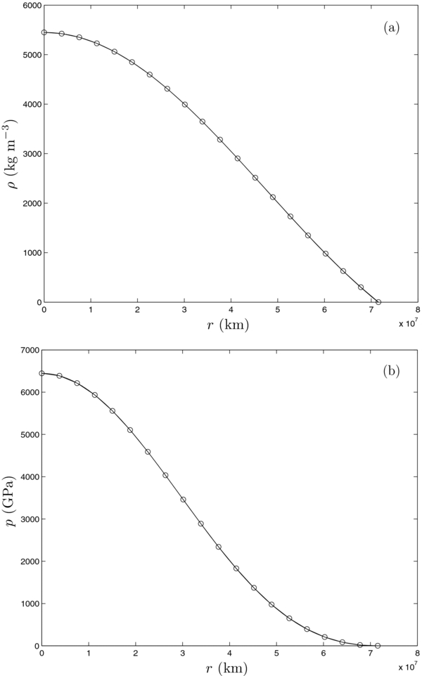
Figure 2. Validation of our numerical solution against the asymptotic solution given by Chandrasekhar (1933): (a) the dependence of ρ on r in the equatorial plane and (b) the dependence of p on r in the equatorial plane. The solid line represents the result of our numerical calculation while the open circles are computed from the analytical expression (34).
Download figure:
Standard image High-resolution image4. NUMERICAL MODELS FOR JUPITER AND α ERIDANI
4.1. Numerical Model for Jupiter
In modeling a rapidly rotating gaseous planet or star, some parameters will be regarded as being well determined by observations while other parameters have to be treated as unknown. In the case of Jupiter, we regard the equatorial and polar radii at the one-bar surface Re
and Rp
—which are Re
= 71, 492 km and Rp
= 66, 854 km (Seidelmann et al. 2007)—as the known parameters. They yield an eccentricity  for the shape of Jupiter. We also regard the rotational period TJ
of Jupiter, TJ
= 9.925 hr (Seidelmann et al. 2007), as a known parameter. This corresponds to the angular velocity ΩJ
= 1.7585 × 10⁻⁴ s−1 for the rotation of Jupiter. The two-dimensional distributions of the density ρ(ξ, η) and the pressure p(ξ, η) within Jupiter are regarded as unknown functions to be determined via our three-dimensional numerical calculation. In addition, the size of K in the EOS p = Kρ2 is also unknown.
for the shape of Jupiter. We also regard the rotational period TJ
of Jupiter, TJ
= 9.925 hr (Seidelmann et al. 2007), as a known parameter. This corresponds to the angular velocity ΩJ
= 1.7585 × 10⁻⁴ s−1 for the rotation of Jupiter. The two-dimensional distributions of the density ρ(ξ, η) and the pressure p(ξ, η) within Jupiter are regarded as unknown functions to be determined via our three-dimensional numerical calculation. In addition, the size of K in the EOS p = Kρ2 is also unknown.
The objective of our numerical calculation is, via a hybrid inverse method, to find the density ρ(ξ, η) and the pressure p(ξ, η) by matching K in the EOS p = Kρ2 with the observed shape  and the observed angular velocity ΩJ
. For a trial value K = KG
and a fixed ΩJ
, we calculate, through the three-stage iterative scheme, an equilibrium solution ρG
satisfying Equation (13) as well as Equations (15) and (16) at a particular value
and the observed angular velocity ΩJ
. For a trial value K = KG
and a fixed ΩJ
, we calculate, through the three-stage iterative scheme, an equilibrium solution ρG
satisfying Equation (13) as well as Equations (15) and (16) at a particular value  at the equilibrium. However,
  is generally inconsistent with the observed value
  for Jupiter. By repeating this process at many different values of KG
, i.e., through an iterative scheme with K, we are able to find a particular value KJ
= KG
such that the shape parameter
for Jupiter. By repeating this process at many different values of KG
, i.e., through an iterative scheme with K, we are able to find a particular value KJ
= KG
such that the shape parameter  is consistent with the observed value
  . In other words, a numerically expensive two-parameter (
 ) iterative process is required in determining the rotationally distorted internal structure of Jupiter.
A relationship between K and  at the equilibrium, resulting from the two-parameter (
 ) iterative process, is shown in Figure 3(a) where the star symbol denotes a particular numerical solution that matches the numerical model with the observed shape of Jupiter
  when K = KJ
= 200, 102 Pa m6 kg−2. In other words, for the fixed rate of rotation ΩJ
and a polytrope of unit index n = 1, the EOS for Jupiter must be of the form
when K = KJ
= 200, 102 Pa m6 kg−2. In other words, for the fixed rate of rotation ΩJ
and a polytrope of unit index n = 1, the EOS for Jupiter must be of the form
in order that its shape matches the observed value  . The detail of the three-stage iterative procedure at K = KJ
is depicted in Figure 3(b). It shows that the function || dVt
/ dη||2 at fixed K = KJ
decreases from || dVt
/ dη||2 = O(1) far away from the equilibrium to || dVt
/ dη||2 = O(10−3) at the equilibrium when reaching the minimum at
. The detail of the three-stage iterative procedure at K = KJ
is depicted in Figure 3(b). It shows that the function || dVt
/ dη||2 at fixed K = KJ
decreases from || dVt
/ dη||2 = O(1) far away from the equilibrium to || dVt
/ dη||2 = O(10−3) at the equilibrium when reaching the minimum at  . Each triangle in Figure 3(b) represents a three-dimensional solution at the fixed KJ
using different three-dimensional finite-element meshes. The particular solution at
. Each triangle in Figure 3(b) represents a three-dimensional solution at the fixed KJ
using different three-dimensional finite-element meshes. The particular solution at  and K = KJ
represents a numerical model for Jupiter with a polytrope of unit index n = 1. Figure 4 shows the density and pressure distribution of this numerical solution in the equatorial plane as well as the eccentricity of constant density surfaces while Figure 5 depicts the two-dimensional density distribution, ρ(η, ξ), in a meridional plane.
and K = KJ
represents a numerical model for Jupiter with a polytrope of unit index n = 1. Figure 4 shows the density and pressure distribution of this numerical solution in the equatorial plane as well as the eccentricity of constant density surfaces while Figure 5 depicts the two-dimensional density distribution, ρ(η, ξ), in a meridional plane.
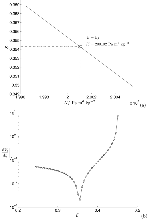
Figure 3. Hybrid inverse method involving a two-parameter ( ) iterative procedure for determining the shape and internal structure of Jupiter. (a) The solid line represents the relationship between K and
  at the equilibrium while the star symbol denotes a particular solution that matches the parameter with the shape of Jupiter at
  when K = KJ
= 200, 102 Pa m6 kg−2. (b) The detail of the three-stage iterative scheme for fixed K = KJ
= 200, 102 Pa m6 kg−2, showing that || dVt
/ dη||2 reaches the minimum at
when K = KJ
= 200, 102 Pa m6 kg−2. (b) The detail of the three-stage iterative scheme for fixed K = KJ
= 200, 102 Pa m6 kg−2, showing that || dVt
/ dη||2 reaches the minimum at  at the equilibrium, where each triangle represents a solution of the three-dimensional numerical simulation at given K = KJ
for different values of
at the equilibrium, where each triangle represents a solution of the three-dimensional numerical simulation at given K = KJ
for different values of  .
.
Download figure:
Standard image High-resolution image
Figure 4. Interior structure from the numerical model of Jupiter: (a) the density ρ, (b) the pressure p, and (c) the eccentricity of constant density surfaces as a function of the radius r in the equatorial plane.
Download figure:
Standard image High-resolution image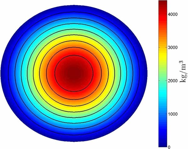
Figure 5. Interior structure from the numerical model of Jupiter: the two-dimensional density distribution ρ(ξ, η) in an oblate spheroid with eccentricity  .
.
Download figure:
Standard image High-resolution imageThe total mass MJ
of Jupiter is MJ
= 1.8986 × 1027 kg (Williams 2010), giving rise to the mean density  . It needs to be emphasized, however, that the Jupiter model with a polytrope of unit index n = 1 does not require an a priori value for the planet's mass. Rather, total mass is determined as part of the three-dimensional numerical solution. This provides a useful constraint on the model whose predicted mass can be compared with the observed mass of Jupiter MJ
. For the two-dimensional density distribution ρ(ξ, η) shown in Figure 5, we find the total mass of our Jupiter model is 100.4% of MJ
. This difference could be attributable to the inadequacy of the n = 1 polytrope to represent the real EOS of the Jovian interior. The zonal gravitational coefficients J2, J4, J6 predicted by the model using the expression (18) are listed in Table 1. Our model predictions of the zonal gravitational coefficients are in reasonably good agreement with observed values (Jacobson 2003) especially when considering that there is only one parameter in the model.
. It needs to be emphasized, however, that the Jupiter model with a polytrope of unit index n = 1 does not require an a priori value for the planet's mass. Rather, total mass is determined as part of the three-dimensional numerical solution. This provides a useful constraint on the model whose predicted mass can be compared with the observed mass of Jupiter MJ
. For the two-dimensional density distribution ρ(ξ, η) shown in Figure 5, we find the total mass of our Jupiter model is 100.4% of MJ
. This difference could be attributable to the inadequacy of the n = 1 polytrope to represent the real EOS of the Jovian interior. The zonal gravitational coefficients J2, J4, J6 predicted by the model using the expression (18) are listed in Table 1. Our model predictions of the zonal gravitational coefficients are in reasonably good agreement with observed values (Jacobson 2003) especially when considering that there is only one parameter in the model.
Table 1. Zonal Coefficients of Jupiter's Gravitational Field
| n | Jn × 106 | Jn × 106 | Jn × 106 |
|---|---|---|---|
| (Model) | (Observed) | (Theory of Figures) | |
| 2 | 14909.60 | 14696.43 ± 0.21 | 14001.53 |
| 4 | −559.07 | −587.14 ± 1.68 | −532.02 |
| 6 | 29.89 | 34.25 ± 5.22 | 31.94 |
Notes. The fourth column is obtained by an application of the Zharkov–Trubitsyn third-order theory of figures to Jupiter (Zharkov & Trubitsyn 1978). The second column is the prediction of our numerical model with 2 × 10⁶ tetrahedral elements and in the third column are observed values (Jacobson 2003).
Download table as: ASCIITypeset image
Our model, which assumes only the size and shape of Jupiter's surface and the planet's rotation rate together with an EOS of the form p = Kρ2, does a reasonable job of predicting the low-order gravitational coefficient J2 of Jupiter with a better than 2% accuracy and the planet's mass with about 4% accuracy. This opens the possibility of inferring the mass and gravitational coefficients of extra-solar bodies whose rotation rates, sizes, and shapes can be measured. Table 1 in the third column also gives values of the zonal gravitational coefficients J2, J4, J6 computed from the theory of figures. They were obtained by an application of the Zharkov–Trubitsyn third-order theory of figures to Jupiter (Zharkov & Trubitsyn 1978), with a polytropic density of index one, an equatorial radius of 71,492 km, and the IAU System III rotation rate of  .
.
The Appendix presents a simplified theory for estimating the value of the polytropic constant K. The theoretical estimate for K from Equation (A4) gives K = 200, 544 Pa m6 kg−2. This estimate is quite close to K = 200, 102 Pa m6 kg−2 obtained by our hybrid inverse method via three-dimensional numerical simulation.
4.2. Numerical Model for α Eridani(Achernar)
Our non-spherical model is particularly suitable for studying the fast rotating B-type star, α Eridani (Harmanec 1988; Perryman et al. 1997), which is strongly distorted by rotational effects. Since the internal pressure in α Eridani is likely radiation-field-dominated, its mean polytropic index n would be larger than unity. We still adopt the polytropic index n = 1 because our main objective is to illustrate a new method of determining the rotationally distorted shape and internal structure from the known or deduced physical parameters of the rapidly rotating star.
Harmanec (1988) estimated, from the luminosity–mass relation of main sequence stars, that the mass of α Eridani is MA
= 6.07 M☉(1.21 × 1031 kg). From spectral line broadening it is deduced that Achernar's rotational speed projected on its equator is Veqsin i = 225 km s−1 (Slettebak 1982), where i is the inclination angle between the rotational axis and the line of sight from the Earth which cannot be observed directly. According to model 4 of Carcifi et al. (2008), which best fits the interferometry observation, the equatorial radius of α Eridani is 10.2 R☉(Re
= 7.10 × 10⁶ km). Using this radius and taking i = 65° (Carcifi et al. 2008), we obtain an angular velocity ΩA
= 3.493 × 10⁻⁵ s−1. In our calculation for α Eridani, we regard its total mass MA
, its equatorial radius Re
, and its angular velocity ΩA
as the known parameters. The two-dimensional distributions of the density ρ(ξ, η) and the pressure p(ξ, η) within α Eridani are regarded as unknown functions to be determined via our three-dimensional numerical calculation. In addition, the shape parameter  and the size of K in the EOS p = Kρ2 are also unknown.
The objective of our numerical calculation for α Eridani is, via a hybrid inverse method, to find the shape parameter  , the density ρ(ξ, η), and the pressure p(ξ, η) by matching K in the EOS p = Kρ2 with the deduced mass MA
. For a trial value K = KG
and a fixed ΩA
, we calculate, through the three-stage iterative scheme, an equilibrium solution ρG
satisfying Equation (13) as well as Equations (15) and (16) at the equilibrium, which gives rise to a particular total mass MG
. However, this size of the mass MG
is generally inconsistent with the value MA
for α Eridani. By repeating this process at many different values of KG
, i.e., through an iterative scheme with K, we are able to find a particular value KA
= 1.8241 × 10⁹ Pa m6 kg−2 such that its total mass MG
is consistent with the value MA
. A relationship between K and M at the equilibrium, resulting from the two-parameter (K−M) iterative process, is shown in Figure 6(a) where the star symbol denotes a particular numerical solution that matches the numerical model with the observed mass of α Eridani MA
at K = KA
= 1.8241 × 10⁹ Pa m6 kg−2. In other words, for the fixed rate of rotation ΩA
= 3.493 × 10⁻⁵ s−1 and a polytrope of unit index n = 1, the EOS for α Eridani must be of the form
, the density ρ(ξ, η), and the pressure p(ξ, η) by matching K in the EOS p = Kρ2 with the deduced mass MA
. For a trial value K = KG
and a fixed ΩA
, we calculate, through the three-stage iterative scheme, an equilibrium solution ρG
satisfying Equation (13) as well as Equations (15) and (16) at the equilibrium, which gives rise to a particular total mass MG
. However, this size of the mass MG
is generally inconsistent with the value MA
for α Eridani. By repeating this process at many different values of KG
, i.e., through an iterative scheme with K, we are able to find a particular value KA
= 1.8241 × 10⁹ Pa m6 kg−2 such that its total mass MG
is consistent with the value MA
. A relationship between K and M at the equilibrium, resulting from the two-parameter (K−M) iterative process, is shown in Figure 6(a) where the star symbol denotes a particular numerical solution that matches the numerical model with the observed mass of α Eridani MA
at K = KA
= 1.8241 × 10⁹ Pa m6 kg−2. In other words, for the fixed rate of rotation ΩA
= 3.493 × 10⁻⁵ s−1 and a polytrope of unit index n = 1, the EOS for α Eridani must be of the form

in order that its mass matches the value MA
= 6.07 M☉(1.21 × 1031 kg). The detail of the three-stage iterative procedure at K = KA
= 1.8241 × 10⁹ Pa m6 kg−2 is depicted in Figure 6(b). It shows that the function || dVt
/ dη||2 at fixed K = KA
decreases from || dVt
/ dη||2 = O(10) far away from the equilibrium to || dVt
/ dη||2 = O(10−2) at the equilibrium when reaching the minimum at  . The particular solution obtained at
  and KA
= 1.8241 × 10⁹ Pa m6 kg−2 represents a numerical model for α Eridani with a polytrope of unit index n = 1. Figures 7(a) and (b) show the density and pressure distribution of this numerical solution in the equatorial plane while the eccentricity of constant density surfaces within α Eridani is shown in Figure 7(c). Figure 8 depicts the two-dimensional density distribution, ρ(η, ξ), in a meridional plane.
and KA
= 1.8241 × 10⁹ Pa m6 kg−2 represents a numerical model for α Eridani with a polytrope of unit index n = 1. Figures 7(a) and (b) show the density and pressure distribution of this numerical solution in the equatorial plane while the eccentricity of constant density surfaces within α Eridani is shown in Figure 7(c). Figure 8 depicts the two-dimensional density distribution, ρ(η, ξ), in a meridional plane.
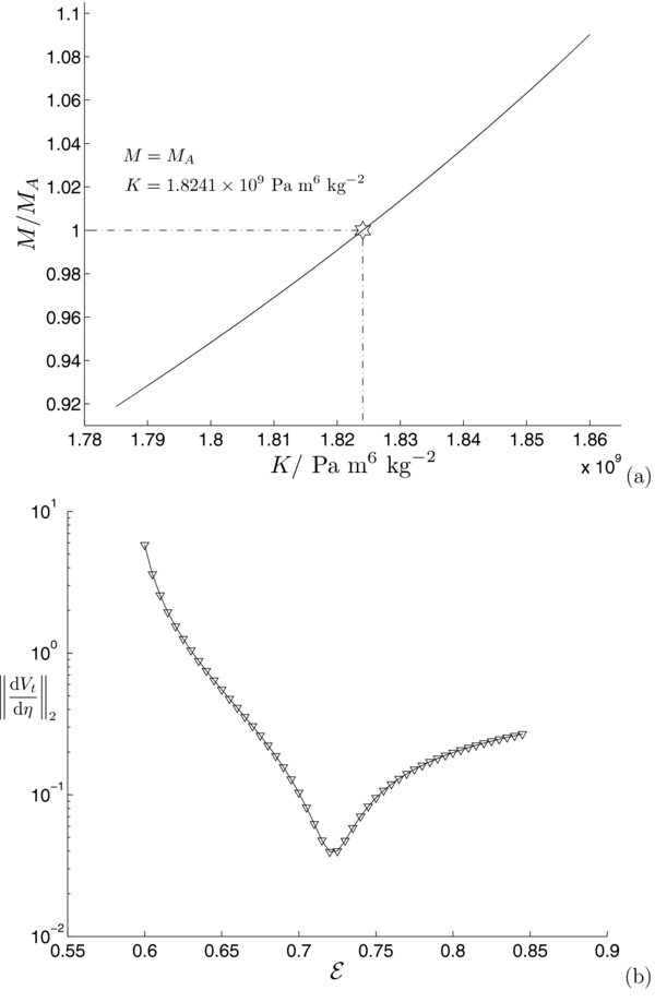
Figure 6. Hybrid inverse method involving a two-parameter (M−K) iterative procedure for determining the shape and internal structure of α Eridani. (a) The solid line represents the relationship between M and K at the equilibrium while the star symbol denotes a particular solution that matches the mass of α Eridani when K = KA
= 1.8241 × 10⁹ Pa m6 kg−2 and  . (b) The detail of the three-stage iterative scheme for fixed K = KA
= 1.8241 × 10⁹ Pa m6 kg−2, showing that || dVt
/ dη||2 reaches the minimum at
. (b) The detail of the three-stage iterative scheme for fixed K = KA
= 1.8241 × 10⁹ Pa m6 kg−2, showing that || dVt
/ dη||2 reaches the minimum at  at the equilibrium, where each triangle represents a solution of the three-dimensional numerical simulation at given K = KA
for different values of the total mass M/MA
.
at the equilibrium, where each triangle represents a solution of the three-dimensional numerical simulation at given K = KA
for different values of the total mass M/MA
.
Download figure:
Standard image High-resolution image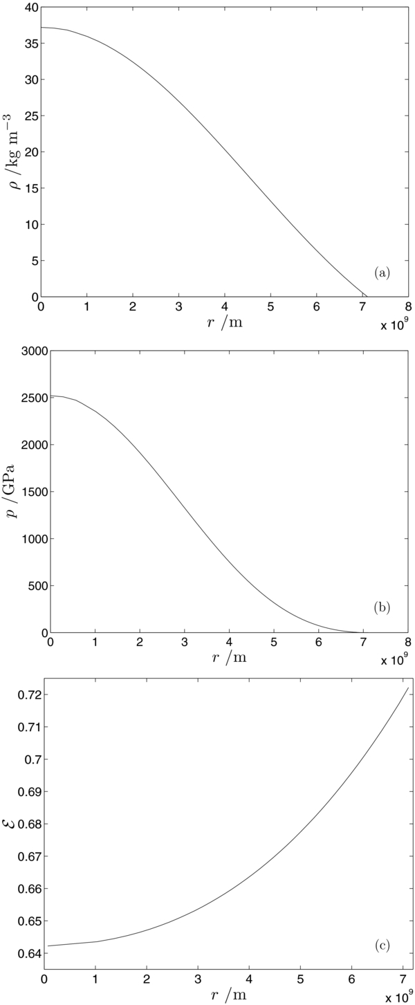
Figure 7. Interior structure from the numerical model of α Eridani: (a) the density ρ, (b) the pressure p, and (c) the eccentricity of constant density surfaces as a function of the radius r in the equatorial plane.
Download figure:
Standard image High-resolution image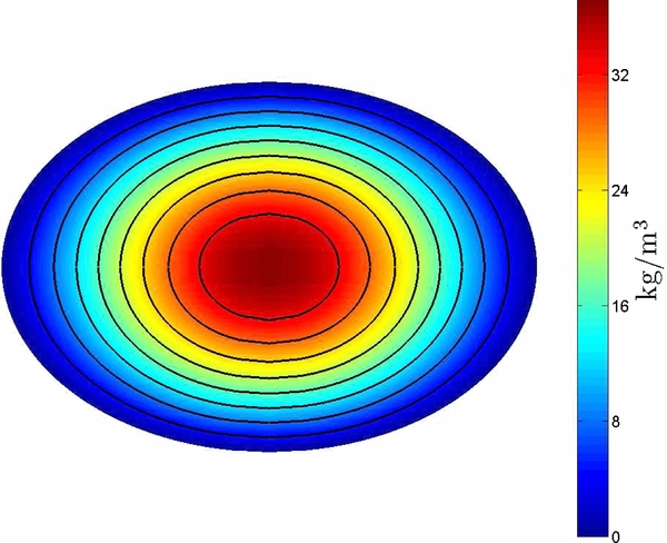
Figure 8. Interior structure from the numerical model of α Eridani: the density distribution ρ(ξ, η) inside α Eridani with the shape parameter  .
.
Download figure:
Standard image High-resolution image
It is found, via our model calculation, that α Eridani must be highly flattened with eccentricity  or Re
/Rp
= 1.45, which is slightly larger than the observational estimate Re
/Rp
= 1.4 (Carcifi et al. 2008). Evidently, perturbation theories based on an expansion using a small rotation parameter around spherical geometry based on
or Re
/Rp
= 1.45, which is slightly larger than the observational estimate Re
/Rp
= 1.4 (Carcifi et al. 2008). Evidently, perturbation theories based on an expansion using a small rotation parameter around spherical geometry based on  are inapplicable to the present problem with
  .
.
5. SUMMARY AND REMARKS
It was nearly 80 years ago that Chandrasekhar (1933) derived the first approximate solution for the internal structure of slowly rotating polytropic planets and stars. An analytical extension of Chandrasekhar's (1933) analysis to rapidly rotating planets and stars proves to be difficult and mathematically challenging. This study is the first attempt to construct a non-spherical numerical model, based on a three-dimensional finite-element method, for the rotationally distorted shape and internal structure of rapidly rotating gaseous bodies with a polytropic index of unity. Our three-dimensional numerical model, which is valid for rapidly rotating objects, is in excellent agreement with Chandrasekhar's (1933) asymptotic solution valid only for slowing rotating planets.
Although the governing mathematical equation of the problem is relatively simple, the numerical procedure for seeking a physically relevant solution to the equilibrium state is quite complicated, intricate, and expensive, involving a two-parameter ( ) iterative procedure for exoplanets or (K−M) iterative procedure for rapidly rotating stars, marked by constructing many different three-dimensional finite-element meshes and carrying out a large number of three-dimensional numerical calculations. This is because a solution to the inhomogeneous Helmholtz equation subject to the simple boundary condition ρ = 0 on the bounding surface
  , which is a priori unknown, is not sufficient. Additionally, the free-surface condition
must be also satisfied on the bounding surface  at the equilibrium. This feature perhaps represents not only the most significant difference between the perturbation theories (Chandrasekhar 1933; Zharkov & Trubitsyn 1978) and the present approach, but also the root of numerical difficulties in this study. It is noteworthy that there exists no simple analytical expression for
when ρ is non-uniform and rotational distortion is too large to be regarded as being a small perturbation (Kong et al. 2010). In other words, any analytical approach for the present problem is likely too complicated to be practically useful.
Evidently, our simple model of a polytrope with unity index n = 1 presented in this paper is not sufficient for the purpose of accurately modeling rotating planets like Jupiter within the tight error bars of the observational constraints. The next necessary step for application to Jupiter and other gaseous planets will include options for more parameters that can be used to adjust the observational constraints such as the total mass of Jupiter.
The method of this paper can be used together with a polytropic EOS with non-unity index or a physical EOS or an empirical EOS. Let us look at the pressure term which is involved in the EOS in the governing equation. First, consider a polytrope with non-unity index n ≠ 1. In this case, the pressure term can be written as
For example, with n = 2 we have
leading to a nonlinear equation for the density ρ which can be solved numerically by a standard iterative method. This is because, for a local method, all differential operators such as  are expressed in terms of local nodes. In the case of a general EOS p = f(ρ), we have
where the coefficient (∂f/∂ρ) can be provided by an EOS that is, for example, in the form of a numerical table between the pressure p and the density ρ. The resulting nonlinear equation can also be solved numerically by the standard iterative method. In other words, the proposed method can be used to deal with any form of the EOS without major mathematical or numerical difficulties.
Rapidly rotating giant planets like Jupiter are marked by the existence of strong zonal flow at the cloud level which may be capable of producing gravitational anomalies if it penetrates sufficiently deep. An extension of the present numerical model by including the effect of a deep zonal flow is underway and will be reported in a future paper.
D.K. is supported by an Exeter University Studentship, K.Z. is supported by UK NERC, STFC, and Leverhulme grants, and G.S. is supported by the National Science Foundation under grant NSF AST-0909206.
: APPENDIX
The hydrostatic equilibrium (HE) equation, which stabilizes internal pressure p(s) with gravitational and rotational forces, can be written (Zharkov & Trubitsyn 1978) as
where r is the mean radius. This equation is valid to the first order in Ω2, the square of the angular velocity of rotation. Higher order terms involve the shape of the surfaces of constant internal potential, the so-called level surfaces at r on the interval 0 ⩽ r ⩽ R, where R is the planet's mean radius at the surface. The internal pressure p is given in terms of the density ρ by an EOS of the form p = f(ρ). When the EOS is given by a polytrope of index one, such that p = Kρ2, with K a constant, the HE equation takes on the particularly simple form of
and the mass mr internal to r is given by the following continuity equation:
An exact solution exists to Equations (A2) and (A3). For a giant planet with polytropic interior, the density, and hence the pressure, are taken as zero at the surface where r = R. The mass at the surface is the total mass MJ . These two boundary conditions yield a unique first-order solution with a mass that is finite, but not necessarily zero at the origin. However, with the mass in the core set to zero, the approximate first-order value of K is unique and it is given by
Basically, the polytropic constant is dependent on the gravitational constant G and the mean radius of the planet R. The smallness parameter q is defined by
For this particular value of K, the density is finite at the center. For larger values of K the central density diverges to positive infinity, while for smaller values it diverges to minus infinity.
Both G and R contribute to the error budget for K. While GMJ
is well determined by spacecraft missions to Jupiter, G itself is relatively poorly determined by laboratory experiments. The recommended 2010 value of G by CODATA
5
is (6.67384 ± 0.00080) × 10−11 m3 kg−1 s−2. In addition to this fundamental physical constant, we adopt astrodynamic constants consistent with the space navigation group at JPL.
6
The equatorial radius of Jupiter at a one-bar level in its atmosphere is 71,492 ± 4 km; the value of GMJ
is 126, 686, 535 ± 2 km3 s−2; and the first two non-zero zonal gravitational coefficients in units of 10−6 are J2 = 14696.43 ± 0.21 and J4 = −587.14 ± 1.68. Using these values and a fifth-order geoid calculation, we obtain a polar radius of 66,854 km and a mean radius of 69,894 km, both uncertain by ± 4 km. The mean density ρ0 of Jupiter, based on its mean radius, is 1327.24 ± 0.26 kg m−3. With a rotation period TJ
of  , the parameter q is 0.083346 ± 0.000014, and the polytropic constant from Equation (A4) is 20,0544 ± 32 Pa m6 kg−2. A numerical integration of the system given by Equations (A2) and (A3) yields a more precise value for K of 200,570 Pa m6 kg−2.
Footnotes
- 5
P. J. Mohr, B. N. Taylor, and D. B. Newell (2011), "The 2010 CODATA Recommended Values of the Fundamental Physical Constants" (Web Version 6.0). This database was developed by J. Baker, M. Douma, and S. Kotochigova. Available at http://physics.nist.gov/constants [Friday, 22-Jul-2011 10:04:27 EDT]. National Institute of Standards and Technology, Gaithersburg, MD 20899, USA.
- 6
Web site http:ssd.jpl.nasa.gov.