A DECADE OF SOLAR TYPE III RADIO BURSTS OBSERVED BY THE NANÇAY RADIOHELIOGRAPH 1998–2008

Particle acceleration events in the quasi-collisionless plasma of the solar corona create supra-thermal electron beams that propagate along magnetic field lines, either away from the Sun into interplanetary space (on so-called open field lines) or downward into the chromosphere (toward the footpoints of magnetic loops). Higher-energy electrons race ahead of the lower energy ones, creating a bump-in-tail instability in the particle distribution. Landau resonance with the unstable electron beams creates Langmuir waves, which are believed to undergo nonlinear wave–wave interaction and produce electromagnetic emissions at the local plasma frequency or its harmonic. As the electron beam propagates to higher or lower altitudes (at speeds of ≈c/3 in the low corona to ≈c/10 at 1 AU; Poquérusse et al. 1996), and hence to lower or higher densities and plasma frequencies, there is a drift in the frequency of emitted radiation. This coherent plasma emission is generally called a type III radio burst. Type IIIs have been observed from frequencies as high as ≈1 GHz at the bottom of the corona to 30 kHz at ≈1 AU, and even lower further out. Taking only bursts drifting from high to low frequencies, Alvarez & Haddock (1973) have fitted bursts in the 74–550 MHz range by the relation (dν/dt) ≈ −0.01 ν^1.84 MHz s⁻¹.

Nita et al. (2002) have investigated the peak flux distributions of 40 years of spatially integrated solar radio burst data, from 0.1 GHz to 37 GHz. They have found that the peak flux density distribution of events, dN/ds_ν followed a power law with a negative index ≈1.8, similar to that found in many X-ray studies (for recent work on the topic, see, e.g., Hannah et al. 2008).

In this work, we have gathered the solar type III peak flux densities, source sizes, and positions at different frequencies, observed by the Nançay Radioheliograph (NRH) over the period 1998 January 1 to 2008 April 1, i.e., covering nearly a full solar cycle.

In Section 2, we describe the data selection process and some of its limitations. We describe the observations in Section 3 and discuss them in Section 4. Finally, in Section 5, we summarize our results and present some conclusions to this study.

We selected our events from the list of solar radio bursts published by the National Oceanographic and Atmospheric Administration's National Geophysical Data Center³ (NOAA/NGDC), from 1998 January 1 to 2008 April 1, covering almost a full solar cycle. We removed all bursts that were outside the observing times and spectral range (∼150–450 MHz) of the NRH (Kerdraon & Delouis 1997). We have not gone further than 2008 April because NRH started observing the Sun with a different set of frequencies, and we wanted a consistent set of frequencies for our statistical study. The NOAA list contains information on individual radio bursts, such as reporting station, start and end times and frequencies, as well as spectral type and intensity. This list is compiled from reports, often generated manually, by observers from various ground stations around Earth (Culgoora, Ismiran, Learmonth, Ondrejov, Palehua, Sagamore Hill, San Vito, Bleien, etc.), using spectrometers covering varying bands, from as low as ∼30 MHz to as high as a few GHz. Hence, certain characteristics such as start and end frequencies, as well as burst intensity, are somewhat subject to both individual spectrometer sensitivity and individual observer's perception. In cases where the same event was reported more than once (by different observatories), only the first such report was kept, and any extraneous ones were ignored. We kept only type III radio burst reports within the times (≈8:30 to 15:30 UT, varying during the year) and the spectral band (150–432 MHz) where the NRH was observing the Sun. Groups of decimetric type IIIs do not last much longer than a few minutes (individual ones last about 1 s). Different groups of type IIIs, even hours apart, are however sometimes bundled together in a single report. Moreover, certain reported time intervals are clearly erroneous, probably due to data entry error. We have therefore ignored all type III reports longer than 10 minutes (which constituted ∼14% of type III reports) and were left with 8931 type III burst reports from 1998 to 2008.

The NRH actually produces images at up to 1/8 s temporal resolution, but these are stored on magnetic tapes, and each individual day of data must be retrieved manually. The 10 s data are stored in a file system, and it is therefore much easier and faster to process. This is the reason why it is used in this study. This coarse temporal resolution leads to weak- and/or short-duration (such as second-long type IIIs) bursts being drowned in the solar background. Hence, we have decided to retain only well-determined type III bursts for this study: those which had peak brightness temperature of 10 MK or above, well above any quiet-Sun value.

This is the case for 91.4% of cases at 164 MHz, down to 26.2% of cases at 432 MHz. The difference is easily explained by the fact that type III bursts tend to have lower brightness temperatures at 432 than at 164 MHz (see also Section 3.3). A priori, the NGDC-reported burst spectral band is not necessarily a good indicator of the actual bandwidth of the type III burst (NRH, possessing ≈44 dishes, is much more sensitive than the single-dish spectrometers that typically report to NGDC). On the other hand, we have empirically observed that taking only bursts either at frequencies for which the peak brightness temperature in the map is above ≈10 MK or within the NOAA-reported spectral range leads to very similar data sets.

The 10 s data used in this study also lead to cases where several individual bursts are being bundled together into a single event. Hence, in this work, a "type III event" is often "a group of type IIIs within the same 10 s interval."

Frequencies 150.9, 164, 236.6, 327, 410.5, and 432 MHz (with a 3 dB bandwidth of 0.7 MHz) were used by NRH during our period of interest.

Figure 1 clearly shows a decrease in radioactivity as the solar cycle approaches minimum, and the dip in events from 2003 November 5 to 2004 January 25 is due to NRH being offline while anti-alias antennas were being added to the array. During our decade of interest, the 150.9 MHz frequency has gradually replaced the nearby 164 MHz, no longer reserved under French law. Hence the observations at 150.9 MHz have started later, with an overlap of a few years with the (now no longer used) 164 MHz. It can be noted that the occurrence rates match qualitatively that of Lobzin et al. (2011), including an almost ∼2 year periodicity, unexplained so far. Using NRH 10 s images, and a fixed 30'' pixel resolution at available frequencies (this standard coarse resolution, still well below the instrumental resolution at 432 MHz, was chosen for ease of data handling), the following were determined (among other things): time of peak flux density, location, and brightness temperature of brightest pixel in the source, and two-dimensional Gaussian fitting parameters to sources present in the image. From the latter, source fluxes can be deduced by computing the Gaussian volume. It is important to note that each frequency was treated mostly independently from each other; see Sections 2.1 and 2.2 for a discussion.

Zoom In Zoom Out Reset image size

Sections 2.1 to 2.6 detail some caveats in our selection and data analysis process.

2.1. Time Interval of Reports

2.2. Alias Ambiguity

2.3. Burst Fluxes

2.4. Astrophysical Sources

2.5. Refractive Effects

We have studied in detail the distribution in spatial sizes (Section 3.1), in positions (Section 3.2), in fluxes (Section 3.3), and the rank-order cross-correlations between several of the observables (Section 3.4).

3.1. Burst Spatial Size Distribution

Radio sources were fitted with two-dimensional elliptical Gaussians. These yield observed Gaussian sizes σ_{a, obs} and σ_{b, obs} (semimajor and semiminor e-folding lengths), and a tilt angle θ_obs of the semimajor axis with respect to the map x-axis (solar east–west). The FWHM values, s_{a, obs} and s_{b, obs}, are obtained by multiplication of σ_{a, obs} and σ_{b, obs} with $2\sqrt{2\ln 2} \approx 2.355$. In Figure 2, we plot a histogram of the rms averages $s_{{\rm rms},{\rm obs}}=\ssty\sqrt{s_{a,{\rm obs}}^2 + s_{b,{\rm obs}}^2}$. The rollover at low source sizes is due to the interferometer beamwidth, which is about 32–55 FWHM at 164 MHz, proportionally smaller at higher frequencies, and varying with the season and time of day.

Zoom In Zoom Out Reset image size

Assuming that the observed source, the interferometer beam, and the true (deconvolved) source were all elliptical Gaussians (with different tilt angles), we have recovered the true source size (see Appendix A for mathematical details), and plotted the results in Figure 3 and their averages in Table 1.

Zoom In Zoom Out Reset image size

Table 1. Mean and Standard Deviation of Observed and Deconvolved (or "True") Source Sizes

Frequency	Observed size	Deconvolved size
(MHz)	(')	(')
150.9	10.9 ± 4.1	5.3 ± 1.8
164	9.7 ± 3.6	4.5 ± 1.6
236.6	7.0 ± 2.7	3.4 ± 1.3
327	5.2 ± 1.9	2.5 ± 1.0
410.5	4.2 ± 1.6	2.1 ± 0.9
432	3.9 ± 1.6	1.9 ± 0.8

Download table as:  ASCIITypeset image

Note that some of the largest events (in size) are probably multiple sources, but it was not the purpose of this statistical work to discriminate between such.

As the spectral indices of the distributions for the bursts selected in Section 2 were very close (from 4.4 to 4.9) at all frequencies, we decided to plot the normalization constants A_ν as a function of frequency. But to remove any normalization issue stemming from the fact that not all frequencies were uniformly employed by NRH during the solar cycle (particularly, 150.9 MHz was used only after 2002 October 28), we have used a slightly smaller subset of our data to which we have fitted similar power laws: we have taken only those events that occurred when NRH was observing at all six frequencies simultaneously, and plotted in Figure 4 the normalization constants A_ν of these new power-law fits. Figure 4 suggests a power-law frequency dependence of the normalization constant A ≈ B ν^β, which has led us to infer that the distribution for true source FWHM size s could be of the form

$$\begin{equation} \frac{\it dN}{\it ds} = B \, \nu ^{\beta } \, s^{\alpha }. \end{equation} \tag{ 1 }$$

We have done two-dimensional fittings of our data, using Equation (1) as model. The fitting parameters (B, α, β) have been found to be moderately dependent on the choice of fitting intervals (and, to a lesser extend, the binning). We therefore prefer to give a range of values for which χ² near unity was obtained: (B, α, β) from (2.0,−3.0,−2.8) to (20.0,−5.0,−3.8), for an average of ≈(7,−4,−3.3) over the 2002–2008 period. The result is in arcmin⁻¹ day⁻¹ if ν is in GHz and s in arcminutes. To account for the factor ≈2 ratio between the 1998–2008 and the 2002–2008 average burst rates (Figure 1), the normalization constant should be changed from 7 to 14 to get a more proper solar-cycle average.

Zoom In Zoom Out Reset image size

When the Sun is low on the horizon during certain period of the year, the beam shape can be extremely asymmetric. To ensure that these extreme cases have not influenced our results, we have therefore run the same study, removing all events occurring in November, December, and January, as well as all events within two hours of sunset or sunrise during February and October. The differences with the above results were negligible.

A more thorough study of source shape and structure, which would address, e.g., cases where more than a single source is present (e.g., Pick et al. 1998, and references therein), is beyond the scope of this paper.

3.2. Radioburst Location

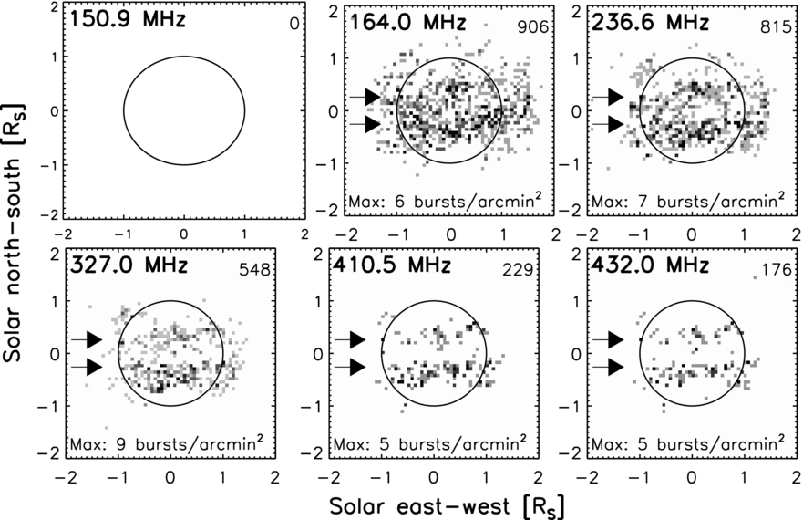
Figure 5 shows the distribution of radio bursts for our selected bursts, using the positions that are likeliest to be correct (as discussed in Section 2), while Figures 6–8 show the same for three different characteristic years in the solar cycle.

Zoom In Zoom Out Reset image size

Zoom In Zoom Out Reset image size

Zoom In Zoom Out Reset image size

Zoom In Zoom Out Reset image size

The most striking feature is, at high frequencies, the concentration of radio bursts in two distinct bands (around latitudes ±15 to ±30° for 432 MHz) during early solar maximum years (Figure 6), and at lower latitudes as the solar cycle advances. This is in remarkable agreement with observed active region and microflare positions and their solar-cycle dependence (e.g., Christe et al. 2008a). Later in the solar cycle, bursts are located mostly south of the solar equator, just as active regions were (Higgins et al. 2012).

The second most striking feature is the systematic shift of about 2' = 120'' westward of the mean position of all radio bursts (Figure 9). While a systematic shift of instrumental origin of up to 03 westward for all frequencies was expected (from comparison between Very Large Array and NRH positions of a radio spike—P. Grigis 2004, private communication), clearly it cannot account for all of the observed shift.

Zoom In Zoom Out Reset image size

3.3. Source Peak Brightness Temperatures and Fluxes

In this section, we investigate the distribution of "peak" (in terms of 10 s averages) brightness temperature T_B (in kelvin) and source fluxes S_ν (in sfu, where 1 sfu = 10⁻²² W m⁻² Hz⁻¹). Figures 10 and 11 show that the peak brightness temperatures and fluxes of our radio bursts follow a (dN/ds_ν)∝S^−1.7_ν law, very close to what Nita et al. (2002) found. Equivalently, the number of bursts above T_B or S_ν follow a power law with negative index one higher (see Figure 12 for S_ν). The rollover at low fluxes is most likely due to our selection criteria (see discussion in Section 2).

Zoom In Zoom Out Reset image size

Zoom In Zoom Out Reset image size

Zoom In Zoom Out Reset image size

Note that unresolved sources always have lower brightness temperature than their "real brightness" temperature, and that a source's "real" brightness temperature is always smaller or equal to its true temperature (opacity). For these reasons, the flux S_ν is probably a less misleading quantity to use than T_B, and we will concentrate on S_ν in the remainder of this section.

As the spectral indices in Figure 11 at different frequencies were very close, we decided to plot the normalization constants A_ν as a function of frequency (Figure 13). As with the source sizes in Section 3.1, we have taken a subset of our data, using only events occurring when NRH was observing with all six frequencies. Power-law fittings to these new distributions yield more meaningful normalization constants A_ν, plotted in Figure 13.

Zoom In Zoom Out Reset image size

Again, note that the coefficients A_ν appear to have a power-law dependence with frequency: A_ν ≈ B ν^β. We have therefore attempted to fit all our data with the following model:

$$\begin{equation} \frac{\it dN}{{\it ds}_{\nu }} = B \, \nu ^{\beta } \, S_{\nu }^{\alpha }. \end{equation} \tag{ 2 }$$

The best-fitting parameters for the 2002–2008 period were found to be (with ν expressed in GHz and S_ν in sfu) B = 0.17 ± 0.01 sfu⁻¹ day⁻¹, α = −1.7 ± 0.05, and β = −2.9 ± 0.1. These fitting parameters have proven to be very stable (and all with near unity χ²) even if changing fitting intervals, and hence much more robust than those found in Section 3.1 for size distributions. To account for the factor ≈2 ratio between the 1998–2008 and the 2002–2008 average burst rates (Figure 1), the normalization constant should be changed from 0.17 to 0.34 to get a proper solar-cycle average.

It is well known that more type III bursts are seen at low frequencies than at high frequencies, and the above relationship reflects this. In fact, Dulk et al. (2001) found the spectrum of a type III burst in the 3–50 MHz range to have a negative spectral index close to 3, in good agreement with our results.

3.4. Rank-order Cross-correlations

We cross-correlated most of the observables mined from our study. The results and method of correlation are described in Appendix E. The only noteworthy relationship that we have observed is the anti-correlation between the "radial elongation" (the ratio of the deconvolved source size in the radial direction over the deconvolved rms source size) of sources and the radial offset from Sun center (Figure 14). This anti-correlation means that sources tend to be circular near disk center, and elliptical near the limb, with minor axis along the radial direction. We will discuss the implications of this mild correlation in the next section.

Zoom In Zoom Out Reset image size

There is a noteworthy absence of strong correlation between the source flux S_ν and the source size s_true, which will also be discussed in Section 4.

Due to the longer path in the corona that emissions from sources near the limb have than those near disk center, it is expected that turbulent scattering would make them appear slightly larger on average than their on-disk brethren (Bastian 1994). There indeed appears to be a slight correlation (≈0.2) between deconvolved source size s_true and angular distance r from Sun center in our data (particularly at the lower frequencies).

Source sizes. The variation of source sizes with frequency relies on a convolution of different effects: the magnetic field structure opening as a function of height in the corona, the fact that we may have several different type IIIs at slightly different locations in the same 10 s time interval, the distribution of intrinsic spatial width of the electron beam (Bastian 1994, considered point sources in his work), and, of course, a host of (mostly refractive in origin) propagation effects (see, e.g., Poquérusse & McIntosh 1995; Dulk 2000, for recent overviews). For example, true source sizes could be 3.5 (harmonic) to 1.7 (fundamental) smaller than observed, according to Melrose (1989).

Average values of type III burst sizes have been measured at frequencies below 169 MHz in the 1970s–1980s (Bougeret et al. 1970; Stewart 1974; Dulk et al. 1979; Dulk & Suzuki 1980). They are found to increase with decreasing frequencies and, on the average, to be of the order of 5' at 169 MHz (values between 2' and 7'; see also Zlobec et al. 1992; Mercier et al. 2006), which compares well with the 45 ± 16 value in Table 1. The first spatially resolved observations of type III bursts at high time resolution with the NRH showed that type III bursts can be resolved into narrow components (Raoult & Pick 1980) (elementary size of the order of 2') with a typical size that increases with time during the burst, potentially reaching 5' to 7' at the end of the burst. What we have measured in the present paper, in which we do not use high time resolution data, will reflect more the total size of the whole type III burst group rather than the size of individual components. Systematic studies of burst sizes have been performed only at 164 MHz (Raoult & Pick 1980; Pick & Ji 1987). The distribution of east–west sizes showed that type III bursts may be resolved in a few cases in components with real sizes around 2', but that the distribution of sizes can reach 9'. The present study provides the first information on the sizes of type III bursts at frequencies above 169 MHz. It shows that type III bursts are smaller at high frequencies than at low frequencies and that the size decreases as ν^−3.3.

Theory (e.g., Bastian 1994, and references therein) predicts that scattering of the emission in the solar atmosphere would lead to a ν⁻² dependence of the source size. This has been confirmed by observations of cosmic sources through the solar corona (Erickson 1964; Coles & Harmon 1989). However, previous observations have showed a quasi-linear dependency of type III source sizes (from ≈0.1 to ≈1500 MHz) with wavelength (Steinberg et al. 1985; Dulk 2000). Our observations support neither.

Although he himself states his analysis becomes invalid for radio wavelengths longer than a few dm, Bastian (1994) predicts a sizable increase of source sizes near the limb. The fact that we seem to observe only a little of it might be an indication that there is a cutoff in the level of turbulence, i.e., that below a certain altitude, turbulence would no longer be proportional to the ambient density as it is for distances greater than 1.7 R_S.

Weak correlation between source sizes and fluxes. This is consistent with the interpretation that emission comes from a spatially small region and that propagation effects (see, e.g., Poquérusse & McIntosh 1995, for a short overview) are responsible for the lack of good correlation. Note, however, that the correlation coefficient gradually improves at higher frequencies (from 0.08 at 164 MHz to 0.35 at 432 MHz), suggesting that these (refractive) propagation effects become less important at higher frequencies.

Source anisotropy near the limb. The slight anisotropy observed as sources get nearer to the limb can be interpreted as being due to the fact that they are being observed more edge-on than when at Sun center, and that the emitting layer is thinner than the horizontal source size.

Source location. Type III emission at the local plasma frequency (fundamental) is expected to be radiated primarily in a dipolar pattern, perpendicular to the local magnetic field. For radiation at the harmonic, a quadrupolar pattern is expected. However, the propagation of radio waves is controlled both by large- and small-scale structures that can modify the primary directivity of the radio emission through respectively refraction (including ducting, Duncan 1979) and scattering processes. Particularly, emission at the fundamental tends to become aligned with the local density gradient. See, e.g., Zheleznyakov & Zaitsev (1970), Melrose (1986), Cairns (1987a, 1987b), and Robinson et al. (1994) for theoretical work; Poquérusse & McIntosh (1995) for a recent short overview; and Thejappa et al. (2012) for recent observational work.

The first investigation of the directivity of type III bursts was achieved by Caroubalos & Steinberg (1974) and Caroubalos et al. (1974) using stereoscopic measurements at 169 MHz obtained simultaneously with the STEREO-1 experiment and with the NRH. Some directivity was found for the type III bursts (especially for the fundamental emission). The directivity was however found to be less than for type I bursts. Stereoscopic measurements of the directivity have then been performed using ground-based measurements at 150 MHZ and measurements on Ulysses in the 1.25–940 kHz range (Poquérusse et al. 1996; Hoang et al. 1997). They found that the average pattern of the type III bursts at low frequencies is shifted 40° eastward of the radial direction. The shift and width is found to decrease with low frequencies. Bonnin et al. (2008) further investigated the directivity of type III bursts in the interplanetary medium using calibrated Wind–Ulysses observations in the same frequency range. They confirmed an eastward shift of 23° at 940–740 kHz and 55° at 55–104 kHz, i.e., increasing with wavelength. In all these papers, the shift is attributed to a transverse density gradient created by the fast wind (propagating along spiraled open field lines) overtaking the (mostly radial) slow wind. At meter wavelengths, an east–west asymmetry for noise storms was reported by Fokker (1960, 1963) and Le Squeren (1963; see Elgarøy 1977, pp. 111–115, and references within for a review). The asymmetry is about 0.1 Rs toward the west. One of the possible explanations that was proposed is that there is a tilt toward the east in the magnetic structures.

In the present study performed at decimetric/metric wavelengths, we do not observe a ∝λ behavior of the westward shift in our data set, but this could be due to the fact that NRH observes bursts at much higher frequencies and much closer to the Sun. On the other hand, combining the observed ≈2' westward shift with a simple geometric model (details in Appendix C), an average tilt angle between the direction of emission and the radial to Sun center can be derived, and has been found to be around 6°. (This result is consistent with a more elaborate model using a Monte Carlo approach, as detailed in Appendix D.) This is in the same order of magnitude as was found from noise storm asymmetries. If one assumes that the optimal direction of emission statistically corresponds to the direction of the local magnetic field, one hence concludes that the magnetic field is on average tilted eastward by ≈6° with respect to the radial direction, at altitudes of a few tenths of a solar radius, where emission at 150–432 MHz occurs.

Derivation of coronal density profile. In the following, we assume that emission is either at the fundamental or the harmonic of the local plasma frequency, though the latter is generally thought to be the dominant emission mechanism in the case of decimetric type III emission. Using position data after 2004 January 25 (the best position data, obtained after the installation of anti-alias antennas), it is possible to derive statistically the average height difference between emission at different frequencies. See Appendix A of Saint-Hilaire et al. (2010) for comprehensive details of the method. This method assumes that sources at different frequencies tend to be radially distributed at different heights. The effect of the small ≈6° tilt angle is neglected. In the first five panels of Figure 15, we have plotted all average R (plane-of-sky, or POS, distance from Sun center) versus ΔR (POS distance between centroid at two different frequencies) for emission at 150.9 MHz versus the other five frequencies. The fitted slopes are proportional to the average height difference (the nearer to disk center, the smaller the height difference, and the nearer to the limb, the larger the height difference). Note that the line must go through the origin, making the fittings much stronger than initially appears. The height differences are plotted in the last panel of Figure 15. We have fitted two simple density profiles to these data.

• 1.  
  A hydrostatic exponential atmospheric n = n₀e^−h/H model (where H is the scale height and h is the altitude above the photosphere), which, in order to be used on our data, is transformed into

  $$\begin{equation} \Delta h_{ij} = h_i-h_j = -2H \ln \frac{\nu _i}{\nu _j}, \end{equation} \tag{ 3 }$$

  where i,j refer to different frequencies of observations. Note that this model is not influenced by whether the emission is at the fundamental or harmonic of the local plasma frequency. Best fitting yields H = 31.5 Mm (the red curve in the bottom plot of Figure 15). This scale height corresponds to a ≈0.6 MK corona, lower than the more usual quiet-Sun values of 1–1.5 MK. This could be due to the fact that we are observing type IIIs near regions of open field lines, and/or the fact that we are near altitudes where solar wind-like conditions start to take over. David et al. (1998) indeed found very low temperatures at similar heights in polar coronal holes.
• 2.  
  A "solar wind-like" atmosphere n(h) = C(h/R_S)⁻² model (Cairns et al. 2009), which, in order to be used on our data, is transformed into

  $$\begin{equation} \Delta h_{ij} = h_i-h_j = 8980 \, m \, R_S \,\sqrt{C} \left(\frac{1}{\nu _i} - \frac{1}{\nu _j} \right), \end{equation} \tag{ 4 }$$

  where m = 1 or 2 for emission either at fundamental of harmonic. The normalization constant C can be viewed as the electron density at an altitude of 1 R_S. Fitting yields C = 5 × 10⁶ cm⁻³ (emission at fundamental) and C = 1.2 × 10⁶ cm⁻³ (emission at harmonic), and the blue curve in the bottom plot of Figure 15. The numbers for harmonic emission are comparatively low, while for fundamental emission, they are comparable to the Baumbach–Allen formula and other published work: e.g., see Newkirk (1961) and Mann et al. (1999) for theoretical models, and see Fainberg & Stone (1974) and Aschwanden & Acton (2001) for a recent compilation of observational work.

Zoom In Zoom Out Reset image size

Note that we have also used the pre-2004 data and have found there was very little difference with the "better" post-2004 data. Both fittings appear equally good (or equally bad), and this methodology cannot decisively choose which of these two models is the most appropriate.

Source intensities and fluxes. Maximum observed brightness temperature T_B in interplanetary type III bursts is reported to be ≈10¹⁵ K, and up to ≈10¹² K for coronal type III bursts (Melrose 1989). We observe a few events >10¹¹ K in our data set.

We have found a power-law dependence of the occurrence rate of type III bursts of peak flux S_ν with a negative spectral index of 1.7, very similar to Nita et al. (2002), and to what is found in X-rays for flare energies (Crosby et al. 1993; Hannah et al. 2008). Eastwood et al. (2010) have found a 2.1 index for interplanetary type III solar radio storm in the 0.125–16 MHz range. A 1.7 negative power-law index is also an oft-seen value in self-organized criticality (SOC) studies: Bak et al. (1988), Lu & Hamilton (1991), Vlahos et al. (1995), Georgoulis & Vlahos (1996), and Aschwanden (2012).

In their study of type I noise storms, Mercier & Trottet (1997) had found negative power-law spectral indices of about 3 to 3.5 for their (dN/ds_ν), and have attributed it to the predicted low-energy part of SOC theory (Vlahos et al. 1995). (Type I noise storm bursts are indeed less energetic but much more frequent than the decimetric type III bursts studied here.) Similarly, Morioka et al. (2007) found a −3.6 index for interplanetary (≈MHz) "micro-type-III" bursts.

Additionally, we find a ∝ν^β (with β ≈ 2.9) spectral dependence of (dN/ds_ν), reflecting the fact that type IIIs are more easily observable, or occur more often, at 164 MHz than at 432 MHz. This exponent could provide constraints to type III emission models such as in Robinson & Cairns (1998) and Melrose (1989).

Solar-cycle-averaged radiative output. To put things in perspective, we compared the global energy radiated by the type III bursts and the energy input of flares into the corona. We have plotted in Figure 16 the "Radio Burst Occurrence Rate" (RBOR) of our observed type IIIs and compared it to the energy input from EUV/X-ray events to the corona, derived in other studies (see, e.g., Hudson 1991, for a discussion on this topic). The RBOR can be estimated from the power-law fitting parameters by using the (dN/ds_ν) at 164 MHz (Figure 11), by assuming a burst bandwidth of Δν ≈ 300 MHz (Isliker & Benz 1994), taking Δt = 10 s (since all our numbers are 10 s averages), and computing the total energy radiated as observed from D = 1 AU. We have further normalized to the photospheric surface area, in order to compare to the "Flare Frequency" often used in coronal heating studies:

$$\begin{equation} {\rm RBOR} = \frac{1}{4\pi R_S^2} \frac{1}{4\pi D^2 \Delta \nu \Delta t}\frac{\it dN}{{\it ds}_{\nu }} \end{equation} \tag{ 5 }$$

(note that 4πD²ΔνΔtds_ν = dE is the radiated energy for one event). The RBOR is hence the occurrence rate of radiated energy distribution of type III events, per unit (photospheric) solar area.

Zoom In Zoom Out Reset image size

One notices that the radiated energy by decimetric type IIIs is about five to six orders of magnitude less than the energy input by EUV nanoflares in the corona (we loosely refer to flares observed in EUV only as "nanoflares," and those observed also in X-rays as "microflares" or "flares"), about the same ratio that exists between the non-thermal hard X-ray emission associated with X-ray flares and microflares, though the emission mechanism is believed to be vastly different (coherent plasma emission versus bremsstrahlung).

Ramesh et al. (2010) have estimated that a 40 sfu metric (77 MHz) interplanetary type III burst was produced by a ≈3 × 10²⁴ erg electron beam. Using the same assumptions on Δν, Δt, and D as before, this would imply an efficiency of non-thermal-radiated energy over beam energy of ≈10⁻⁵ (within an order of magnitude). It is interesting to note that this ratio is somewhat similar to the one between radiated non-thermal X-rays and the energy in thick-target (Brown 1971) accelerated electrons (see Appendix B). To our present knowledge, there is no obvious reason for the non-thermal bremsstrahlung efficiency (an incoherent process) and the efficiency of type III plasma emission (a collective process) to be similar, and it may be a coincidence. Clearly, more studies are needed to ascertain radiative efficiencies, but assuming that they are indeed similar, this has the consequence that nanoflare and possibly microflare electrons could be similar in number and energies to type III-producing escaping coronal electron beams! This is in contradiction with recent studies (Christe et al. 2008b; Saint-Hilaire et al. 2009), which have shown that there is probably a factor of ≈500 more flare electrons than escaping electrons. However, note that these studies were centered on one-to-one association of precipitating flare electron beams and escaping interplanetary electron beams (loosely assuming that interplanetary beams and their counterparts in the low corona have similar properties), while the present study is more global (and, for example, it allows for temporal displacement between the two phenomena and different rates of occurrence). One of the implications is that escaping electron beams carry energy away from the corona, partially or wholly negating coronal heating by nanoflares. We dare not speculate any further without a better handle on radiative efficiencies of type III-producing electron beams. The upcoming NuStar mission (Harrison et al. 2005), and perhaps also the FOXSI rocket flight (Krucker et al. 2009), should reveal how many electrons are in type III beams (via their X-ray emission), yielding the efficiency of type III radio emission.

We have studied solar type III radio bursts observed by NRH during 1998–2008, almost a full solar cycle. From this very rich data set, we have determined source sizes, locations, fluxes, and their frequency distributions.

The source size distribution dN/ds can be fitted with a double power law in ν and in s. The type III burst sizes are found to decrease as ν^−3.3, which could reflect a combination of the magnetic field opening as a function of height in the corona, and the distribution of the spatial widths of electron beams in the corona.

The source flux distribution follows a −1.7 power law at all frequencies. A two-dimensional power-law fitting yields (dN/ds_ν)∝ν^−2.9 S^−1.7_ν. These values offer additional constraints to theoretical models of type III emission.

Type III emission generally comes from active regions (just as flares), and we have observed an east–west asymmetry in their location, which could be explained by an eastward tilt of the magnetic field (compared to the local radial to Sun center) at the typical height where our metric/decimetric type III emission occurred. We have estimated that the tilt angle is ≈6° at altitudes ≈0.3–0.6 R_S.

A barometric fit to the data led to a ∼32 Mm scale height, and temperatures similar to what can be found in coronal holes, while fitting a solar-wind-like density profile yielded a density of (5 × 10⁶)/m² cm⁻³ (where m is the harmonic number) at an altitude of 1 R_S.

Furthermore, we speculated that the solar-cycle averaged radiated type III energy output could be similar to that of radiated non-thermal bremsstrahlung from accelerated nanoflare electrons.

We further suggest that escaping electron beams could be a viable mechanism for carrying energy away from the corona, in a quantity similar to the energy introduced into it through nanoflares, though this result depends heavily on as yet ill-known radio radiative efficiencies.

It is likely that statistical testing of the different theoretical models of the generation and propagation of type III bursts (e.g., Dulk et al. 1979; Duncan 1979; Robinson & Cairns 1998) could be performed, in particular, refractive effects on apparent source sizes, locations, and fluxes. Possible other future work includes the usage of sub-second or the full 128 ms resolution data, if it ever becomes easily usable (e.g., stored on a file system instead of on tapes). After the development of a good (and automated) type III burst detection and discrimination (e.g., Lobzin et al. 2009), this work could be repeated almost verbatim. In the meantime, it is envisaged to do a statistical comparison between the type III bursts in this work and the X-ray flare parameters found in the RHESSI flare or microflare lists, and to obtain observational constraints on radiative efficiencies by comparing them with in situ measurements of electron beams associated with the metric/decimetric type III emissions presented in this work.

We thank the referee for thoughtful comments on this manuscript. P.S.H. was supported by NASA Heliospheric Guest Investigator grant NN07AH74G and NASA Contract No. NAS 5-98033. The NRH is funded by the French Ministry of Education, the French program on Solar Terrestrial Physics (PNST), the Centre National d'Etudes Spatiales (CNES), and the Région Centre. M.V. and A.K. acknowledge support from the CNES and the PNST. Special thanks to Anne Bouteille, Gordon Hurford, Hugh Hudson, Säm Krucker, and Jim McTiernan for discussions pertaining to this and other related work.

Facility: NRHA - Nancay Radio Heliograph Array.

The convolution of a Gaussian elliptical source (semimajor axis a_true, semiminor axis b_true, and tilt angle θ_true) with a Gaussian elliptical beam (a_beam, b_beam, θ_beam) yields an observed source that is also an elliptical Gaussian (a_obs, b_obs, θ_obs). Through Fourier transformation, the following can be derived:

$$\begin{eqnarray} && \tan (2 \, \theta _{{\rm true}}) \nonumber\\ &&\quad = \frac{ \big(a_{{\rm obs}}^2 - b_{{\rm obs}}^2 \big) \, \sin (2 \, \theta _{{\rm obs}}) - \big(a_{{\rm beam}}^2 - b_{{\rm beam}}^2 \big) \, \sin (2 \, \theta _{{\rm beam}}) }{ \big(a_{{\rm obs}}^2 - b_{{\rm obs}}^2 \big) \, \cos (2 \, \theta _{{\rm obs}}) - \big(a_{{\rm beam}}^2 - b_{{\rm beam}}^2 \big) \, \cos (2 \, \theta _{{\rm beam}}) } \nonumber\\ \end{eqnarray} \tag{ A1 }$$

$$\begin{eqnarray} a_{{\rm true}} & = & \sqrt{ \frac{1}{2} \big(a_{{\rm obs}}^2 + b_{{\rm obs}}^2 - a_{{\rm beam}}^2 - b_{{\rm beam}}^2 + \Delta \big) } \end{eqnarray} \tag{ A2 }$$

$$\begin{eqnarray} b_{{\rm true}} & = & \sqrt{ \frac{1}{2} \big(a_{{\rm obs}}^2 + b_{{\rm obs}}^2 - a_{{\rm beam}}^2 - b_{{\rm beam}}^2 - \Delta \big) } \end{eqnarray} \tag{ A3 }$$

with

$$\begin{eqnarray} &&\Delta = \frac{ \big(a_{{\rm obs}}^2 - b_{{\rm obs}}^2 \big)\,\cos (2\,\theta _{{\rm obs}}) - \big(a_{{\rm beam}}^2 - b_{{\rm beam}}^2 \big)\,\cos (2\,\theta _{{\rm beam}}) }{ \cos (2\,\theta _{{\rm true}})} \nonumber\\ \end{eqnarray} \tag{ A4 }$$

$$\begin{eqnarray} &or&\; \Delta = \frac{ \big(a_{{\rm obs}}^2 - b_{{\rm obs}}^2 \big)\,\sin (2\,\theta _{{\rm obs}}) - \big(a_{{\rm beam}}^2 - b_{{\rm beam}}^2 \big)\,\sin (2\,\theta _{{\rm beam}}) }{ \sin (2\,\theta _{{\rm true}})} \nonumber\\ \end{eqnarray} \tag{ A5 }$$

(use whichever has a non-zero denominator).

Moreover, an important result, which can be derived by combining Equations (A2) and (A3), is

$$\begin{equation} s_{{\rm obs}}^2 = s_{{\rm true}}^2 + s_{{\rm beam}}^2, \end{equation} \tag{ A6 }$$

where s²_i = a_i² + b²_i, with i being obs, true, or beam, i.e., when dealing with the convolution of elliptical Gaussians, the rms size of the observed source is simply the quadratic mean of the rms size of the beam and of the true source, independent of any tilt angle between the true source and the beam.

For an injected electron spectrum with negative spectral index δ and low-energy cutoff E_c, and assuming non-relativistic cross-sections for bremsstrahlung (Bethe–Heitler) and energy losses, the ratio of total emitted X-ray energy over accelerated electron energy can be approximated by the following analytical expression, derived by considering the photon spectrum to be a power law above a low-energy cutoff E_c, and a flat spectrum below it:

$$\begin{equation} \eta \approx \frac{4}{3\pi }\frac{\alpha }{\Lambda } \overline{z^2} \frac{1}{m_ec^2} \frac{B(\delta /2,1/2)}{\delta -1} f^{-\delta +2} \left(1 + \frac{f E_c}{\delta -3} \right), \end{equation} \tag{ B1 }$$

where α is the fine structure constant (≈1/137), Λ is the Coulomb logarithm (≈20–30 for fully ionized coronal plasma), $\overline{z^2}$ is the average coronal atomic number-squared (≈1.44), m_ec² = 511 keV, B is the Beta function, δ is the electron flux power-law negative spectral index, E_c is the low-energy cutoff expressed in keV, and f is a slowly varying function that depends mostly on δ and is equal to about 0.3 for δ = 4. For example, for δ = 4 and E_c = 10 keV, one gets a bremsstrahlung emission efficiency of 8.5 × 10⁻⁶. We have found good (within a 10%–20%) correspondence with (exact) numerical computations.

From the observation that radio sources seem to be displaced westward by ∼2' on the average, we derive an average tilt angle of the magnetic field (or at least the direction of the main type III emission) with the local radial to Sun center.

For simplicity, we consider in the following the geometry to be wholly within the ecliptic plane, and the type III emission to have infinite directivity (zero beamwidth).

The "average" source is observed to be at a westward angle χ from Sun center (χ ≈ 2'), at an altitude R_S + h, where R_S is the solar radius. We call ϕ the angle between the Sun–Earth line and the radial to the source, and α the angle between the radial to the Sun and the direction in which the type III is emitted (Figure 17).

Zoom In Zoom Out Reset image size

Then, the following must be true for the emission from the "average" source (which is near the solar surface) to be observed at Earth:

$$\begin{equation} \alpha = \phi + \chi. \end{equation} \tag{ C1 }$$

A bit of trigonometry yields

$$\begin{equation} \sin (\phi) = \frac{ D - (R_S+h) \cos (\phi)}{R_S+h} \tan (\chi), \end{equation} \tag{ C2 }$$

where D is the Sun–Earth distance (≈215 R_S). This is a transcendental equation which can be iteratively solved for ϕ. α is then simply derived from Equation (C1). The following explicit formula, derived using simplified geometry,

$$\begin{equation} \alpha \approx \chi + \arcsin \left(\frac{\chi \cdot D}{R_S+h}\right) \end{equation} \tag{ C3 }$$

has accuracy better than 1% for h ⩽ 0.6R_S.

Using χ = 2', and for h between 0.1 and 0.5 R_S (approximate altitude up to which decimetric emission can be found, cf. Figure 9), one obtains α between 66 and 48. Say α = 6° ± 1°.

These results were derived from a very simple two-dimensional model, assuming that the type III emission had infinite directivity, but they are in good agreement with the Monte Carlo approach presented in Appendix D.

In addition to the simple geometrical approach described in Appendix C, we ran a simple three-dimensional simulation to estimate the effects of a tilt angle α of the radio emission with respect to the local radial, the half-width Δα of the cone of emission, and the source altitude h. One hundred thousand sources were uniformly distributed in longitude, but only within 15° and 30° in latitude (which reflects reality). For each source, if Earth (and the observer) was within the cone of emission, the apparent position of the source on the Sun was recorded. If not, it was omitted. In Figure 18, we display the variations in averaged source east–west position if one varies α, Δα, or h.

Zoom In Zoom Out Reset image size

Using canonical values of α = 6°, Δα = 30°, and h = 0.5 R_S, one obtains a westward displacement of 137'', i.e., very close to our reported observations. It can be said from Figure 18 that the result does not strongly depend on the exact value of h, i.e., a change of 0.1 R_S leads to a change of the average displacement by ≈10''. Reasonable (<80°) values of Δα lead to variations of up to ±25'' at the most.

We conclude that the 6° ± 1° tilt angle obtained in Appendix C is further validated by the simple three-dimensional model presented in this appendix.

Table 2 displays the Spearman Rank-order cross-correlation coefficients between burst parameters, for bursts observed at 164, 327, and 432 MHz. Spearman's Rank-order cross-correlation acts on the ranking of the values instead of on their actual values, as a regular cross-correlation (e.g., Pearson's) would. This has the huge advantage that even a nonlinear (polynomial, exponential, power law, etc.) relationship between parameter x and parameter y can achieve a cross-correlation coefficient near unity. The parameters are

• 1.  
  r is the angular distance to Sun center;
• 2.  
  T_{B, true} is the peak brightness temperature (averaged over 10 s) of the deconvolved Gaussian source (as described in Figure 10 and Section 3.1);
• 3.  
  S_ν is the burst flux (averaged over 10 s);
• 4.  
  s_true is the FWHM size of the source, deconvolved as explained in Section 3.1;
• 5.  
  θ_true is the orientation of the semimajor axis of the source, from the map x-axis;
• 6.  
  (a/b)_true is the ratio of the semimajor to semiminor axis of the source, an easier quantity to visualize than the eccentricity;
• 7.  
  s_{true, radial}/s_true is a measure of the source's radial elongation, normalized to source rms size;
• 8.  
  s_{true, azimuthal}/s_true is a measure of the source's azimuthal elongation, normalized to source rms size.

Table 2. 164, 327, and 432 MHz Rank-order Cross-correlations between Parameters

	r	TB, true	Sν	strue	θtrue	(a/b)true	$\frac{s_{{\rm true,rad}}}{s_{{\rm true}}}$	$\frac{s_{{\rm true,azim}}}{s_{{\rm true}}}$
164 MHz
r	1.00	−0.16	−0.07	0.28	0.00	0.18	−0.37	0.37
TB, true	−0.16	1.00	0.90	−0.16	−0.00	−0.01	0.13	−0.02
Sν	−0.07	0.90	1.00	0.08	0.02	0.01	0.01	−0.01
strue	0.28	−0.16	0.08	1.00	0.07	0.31	−0.13	0.24
θtrue	0.00	−0.00	0.02	0.07	1.00	0.06	0.01	−0.02
(a/b)true	0.18	−0.01	0.01	0.31	0.06	1.00	−0.34	0.45
strue, radial/strue	−0.37	0.13	0.01	−0.13	0.01	−0.34	1.00	−0.89
strue, azimuthal/strue	0.37	−0.02	−0.01	0.24	−0.02	0.45	−0.89	1.00
327 MHz
r	1.00	−0.06	0.07	0.21	0.01	0.05	−0.34	0.34
TB, true	−0.06	1.00	0.77	−0.21	−0.00	−0.06	0.11	0.00
Sν	0.07	0.77	1.00	0.29	0.04	0.01	−0.01	0.01
strue	0.21	−0.21	0.29	1.00	0.07	0.25	−0.05	0.16
θtrue	0.01	−0.00	0.04	0.07	1.00	−0.00	−0.01	−0.00
(a/b)true	0.05	−0.06	0.01	0.25	−0.00	1.00	−0.22	0.34
strue, radial/strue	−0.34	0.11	−0.01	−0.05	−0.01	−0.22	1.00	−0.89
strue, azimuthal/strue	0.34	0.00	0.01	0.16	−0.00	0.34	−0.89	1.00
432 MHz
r	1.00	−0.04	0.11	0.18	−0.02	0.05	−0.32	0.29
TB, true	−0.04	1.00	0.71	−0.19	−0.03	−0.07	0.17	−0.00
Sν	0.11	0.71	1.00	0.35	0.04	−0.03	0.03	−0.00
strue	0.18	−0.19	0.35	1.00	0.04	0.23	−0.03	0.20
θtrue	−0.02	−0.03	0.04	0.04	1.00	−0.01	−0.01	−0.02
(a/b)true	0.05	−0.07	−0.03	0.23	−0.01	1.00	−0.18	0.35
strue, radial/strue	−0.32	0.17	0.03	−0.03	−0.01	−0.18	1.00	−0.83
strue, azimuthal/strue	0.29	−0.00	−0.00	0.20	−0.02	0.35	−0.83	1.00

Download table as:  ASCIITypeset image