


ABSTRACT
The structure of non-force-free equilibrium magnetic flux ropes in an ambient medium of specified pressure pa is studied. A flux rope is a self-organized magnetized plasma structure consisting of a localized channel of electric current and the magnetic field arising from this current. An analytic method is developed to obtain one-dimensional equilibrium solutions satisfying c−1J × B − ∇p = 0 subject to the requirements that (1) all physical quantities be nonsingular and continuous, (2) pressure p(r) be physically admissible—real and non-negative, and (3) the magnetic field profile have "minimum complexity." The solutions are shown to be characterized by two parameters,  and B*p ≡ Bpa/(8πpa)1/2, where
  is the toroidal (axial) field averaged over the cross-sectional radius a and Bpa is the poloidal (azimuthal) field at the edge of the current channel (r = a). The physical constraint on pressure defines equilibrium boundaries in the B*t–B*p space beyond which no physical solutions exist. The method is illustrated with a number of families of solutions governed by distinct physical constraints. The force-free limit with pa ≠ 0 is investigated and is found to be characterized by plasma β = ∞. The local Alfvén speed VA and plasma β are computed. The results are scale-invariant.
Export citation and abstract BibTeX RIS
1. INTRODUCTION
Magnetic flux ropes are important building blocks of the solar corona and interplanetary medium. A flux rope is a self-organized magnetized plasma structure consisting of an electric current distribution J(x) and its magnetic field B(x) embedded in an ambient medium of pressure pa. The magnetic field enables a flux rope to maintain its structural identity separate from the ambient plasma. Remote solar observations show that well-defined loop-like density features are ubiquitous in the corona on a wide range of scales (e.g., Bray et al. 1991). Their underlying magnetic structure is thought to be that of flux ropes. Flux ropes likely exist in the convection zone (e.g., Parker 1979; Spruit 1981; Chou & Fisher 1988), and possible observational signatures of flux ropes rising through the photosphere have been reported (Tanaka 1991; Lites et al. 1995; Leka et al. 1996) and numerically simulated (Fan & Gibson 2003; Manchester 2007; Cheung et al. 2010). By implication, flux ropes are expected to play similar roles in stellar atmospheres (Haisch 1989). In interplanetary space, the characteristic magnetic features of flux ropes have been identified in in situ solar wind (SW) magnetic field and plasma data at various heliocentric distances extending to ∼5 AU (e.g., Burlaga et al. 1981; Marubashi 1986, 1997; Lepping et al. 1990; Bothmer & Schwenn 1994; Liu et al. 2005). Such SW structures, referred to as "magnetic clouds", or MCs (Burlaga et al. 1981), have been inferred to result from the ejecta of coronal mass ejections (CMEs) based on observations (Burlaga et al. 1981) and theory (Chen & Garren 1993; Chen 1996; Wu et al. 1999). Some observed MCs have been directly traced to specific CME eruptions (Kunkel & Chen 2010) using coordinated remote and in situ observations by the Solar Terrestrial Relations Observatory satellites, supporting the above observational and theoretical conclusions. It has long been known that large sporadic (i.e., nonrecurrent) geomagnetic storms are driven by strong and well-organized (i.e., long-duration) southward interplanetary magnetic fields (e.g., Rostoker & Fälthammar 1967; Russell et al. 1974; Perreault & Akasofu 1978; Gonzalez & Tsurutani 1987). Solar flux ropes provide the most important source of such magnetic fields. There is observational evidence that there are flux ropes in the magnetosphere (e.g., Linton & Moldwin 2009). In laboratory systems, various pinches such as the Bennet pinch (Bennett 1934) and tokamak plasmas (Shafranov 1966) constitute examples of laboratory flux ropes.
In natural plasma environments, flux ropes reside in background plasmas. They are generally curved, with the local geometry characterized by major radius R and minor radius a. The forces on the flux ropes are balanced by the ambient pressure. For R/a ≫ 1, the minor radial forces can be approximated by those acting on a straight cylinder (e.g., Shafranov 1966). Although this approximation incurs an error of  and becomes less accurate as R/a approaches unity, the simple configuration can capture the essential structure of flux ropes. As a result, a large body of literature exists dealing with the internal radial structure of flux ropes in one dimension (1D) (e.g., Gold & Hoyle 1960; van Hoven et al. 1977; Marubashi 1986; Burlaga 1988; Chen 1996).
Within the framework of magnetohydrodynamics (MHD), the internal structure of an equilibrium flux rope in the absence of gravity is determined by (1/c)J × B = ∇p, where J = (c/4π)∇ × B. A particular limiting case, the so-called force-free (FF) approximation defined by c−1J × B = ∇p = 0, has been extensively used because of its mathematical simplicity. For B = |B| ≠ 0, this approximation implies J∥B everywhere so that any field of the form J = α(x)B embedded in a p( x) = const medium can satisfy J × B = 0, where α(x) is a scalar function. A number of FF and piecewise FF solutions have been used to model solar flux ropes including the so-called Gold–Hoyle model (Gold & Hoyle 1960), and the constant-α Lundquist (1950) solution has been used to fit the field profiles of observed MCs (e.g., Burlaga 1988; Lepping et al. 1990; Bothmer & Schwenn 1994; Marubashi 1997). The Lundquist solution is a special case of the more general FF equilibria with non-constant α (e.g., Lüst & Schlüter 1954). These are highly constrained solutions in that J(x) and B(x) are required to satisfy a specific functional form and relationship at every spatial point.
The macroscopic constraint, α = const, can be justified in certain confined laboratory systems by conjecturing that local dissipation (via, reconnection) destroys the magnetic flux surfaces so that α(x) becomes independent of space (Taylor 1974). This assumption has led to a satisfactory explanation for the structure of reverse field pinches (RFPs) in the laboratory, a magnetically confined configuration maintained by an external coil producing a strong toroidal field and induced toroidal current. In general, however, plasma configurations need not relax to this so-called Taylor state (e.g., Zhu et al. 1995). Indeed, tokamak equilibria (Shafranov 1966), which exhibit ∇p ≠ 0, do not relax to an FF state because their magnetic surface properties are different from those of Taylor's RFP configuration. Furthermore, in an ideal MHD system or where dissipation is negligible on the dynamical time scale, a magnetized plasma structure need not relax to a constant-α Taylor configuration.
Previously, a number of non-force-free (NFF) configurations have been discussed in the solar and SW literature (e.g., van Hoven et al. 1977; Chen 1996; Hu & Sonnerup 2002; Hidalgo et al. 2002; Romashets & Vandas 2004; Petrie 2008). In van Hoven et al. (1977), magnetic field profiles in 1D flux ropes with prescribed pressure profiles, p(r), were calculated. In Chen (1996), an NFF magnetic field of a flux rope expanding past an observer was obtained to describe the essential characteristics of MCs. In this work, the expansion of the minor radius a(t) was derived from a dynamical model of flux-rope expansion, producing asymmetry in the field profile resembling that in the observed MCs, but the pressure profile was not calculated. Hidalgo et al. (2002) constructed an NFF configuration and compared it with the magnetic field profiles of a number of observed MCs. The flux rope was assumed to have a circular cross-section, and no expansion was included. Romashets & Vandas (2004) considered an NFF configuration in which the observed asymmetry in MC fields was modeled using non-concentric flux surfaces. Although all of these models used NFF magnetic fields, none of them included pressure or self-consistently calculated pressure profiles. One exception is the work of Hu & Sonnerup (2002) who treated MCs as straight cylinders with non-circular cross-sections and solved the Grad–Shafranov equation given a pressure profile of the form p(A), where A is the vector potential. Another exception is the work of Petrie (2008) who investigated both FF and NFF profiles in two dimensions using separable solutions of the Grad–Shafranov equation with azimuthal symmetry (∂/∂θ = 0, ∂/∂z ≠ 0). Numerical simulations of the structure and dynamics of NFF flux ropes in the solar (and stellar) convection zone have also been carried out (e.g., Moreno-Insertis & Emonet 1996; Fan 2001; Archontis et al. 2004; Arber et al. 2007).
In the present paper, we extend the previous 1D treatments of flux ropes to NFF equilibria and self-consistently and analytically solve c−1 J × B − ∇p = 0, calculating B(r) and p(r) for specified asymptotic ambient pressure pa, average toroidal field  , and poloidal field Bpa at the edge of the current channel (r = a). The ability to find equilibrium solutions to satisfy specified conditions is important because (1) in a dynamical environment, a flux rope evolves through an ambient medium that is determined by processes external to the flux rope and (2) an initial structure need not evolve into an FF flux rope. Furthermore, we impose requirements that (1) physical quantities be everywhere continuous and nonsingular, (2) pressure p(r) be real and non-negative (and smoothly converge to the ambient value pa), and (3) the magnetic field profile have "minimum complexity." No specific radial dependence of p(r) or B(r) is prescribed. It is shown that the solutions can be specified by two parameters,
  and B*p ≡ Bpa/(8πpa)1/2, where
  is the toroidal (locally axial) field averaged over the minor radius and Bpa is the poloidal (locally azimuthal) field at the edge of the current channel, r = a. Furthermore, the requirement of real and non-negative pressure defines equilibrium boundaries beyond which no physical equilibrium solutions exist. It is also shown that solutions can be obtained by imposing the additional conditions that physical quantities be not only continuous but differentiable and the average pressure inside the current channel be equal to a specified value. Each set of constraints leads to a distinct family of solutions. The non-negative pressure condition leads to a similar equilibrium boundary for the Gold–Hoyle solution. The MHD equilibrium properties discussed in the present paper are scale-invariant.
It is often stated that plasma β ≡ 8πp/B2 in the solar corona is so small that pressure may be regarded as negligible, allowing one to use the FF approximation, c−1J × B = ∇p = 0. Having no rigid confinement walls, however, a magnetized structure in the corona ultimately requires coronal plasma pressure for force balance. Thus, small β does not imply ∇p = 0. More to the point, β → 0 means p/B2 → 0, whereas "force free" means |∇p| = 0, which can be satisfied by any p( x) = const. This means that β is indeterminate for a truly FF structure ( J × B = 0 for all x). For any pa ≠ 0, both low-β and high-β NFF solutions are possible, with |dp/dx|max ranging from 0 to ∞. Analytic solutions will be presented to demonstrate these properties. Formally, for a flux rope restricted to a finite extent (r ⩽ a) in an ambient medium of pressure pa, it will be seen that the FF limit corresponds to β → ∞. These limiting properties arise because p( x) and B( x) must satisfy force balance with the ambient pressure. Under some physical conditions, no FF limit exists.
The organization of this paper is as follows. In Section 2, the basic equilibrium equation and the physical constraints on the system are discussed. Section 3 presents the general solutions and the equilibrium boundary for physical solutions. Three particular families of solutions subject to different constraints are discussed in Sections 3.1–3.3. The FF limit of the present solutions is examined and compared with the well-known Gold–Hoyle and Lundquist solutions in Section 4. The work is summarized in Section 5.
2. ONE-DIMENSIONAL NON-FORCE-FREE (NFF) FLUX ROPES
In equilibrium the applicable MHD equations are

where gravity is neglected. We use a cylindrical coordinate system with the axis of the flux rope aligned with the z (toroidal) direction, as illustrated in Figure 1. The radial coordinate measured from the axis of the cylinder is r, with the electric current J limited to r ⩽ a. The poloidal (locally azimuthal) angle is denoted by θ. The treatment is one dimensional, and we impose ∂/∂z = ∂/∂θ = 0. Pressure is p(r) with the ambient pressure pa ≠ 0 taken to be constant, consistent with the neglect of gravity.

Figure 1. Schematic of a flux rope in equilibrium with ambient pressure pa. The cylindrical coordinates θ and z are shown. The radial coordinate is measured from the axis at r = 0. The edge of the current channel is at r = a. Toroidal (poloidal) magnetic field component Bt (Bp) is shown. The "flux rope" consists of the current channel and the magnetic field produced by the current. The plasma β is typically much smaller inside than outside the flux rope.
Download figure:
Standard image High-resolution imageThe current density has components Jp(r) and Jt(r) in the poloidal and toroidal directions, producing toroidal Bt(r) and poloidal Bp(r) magnetic field components, respectively. Because of the assumed cylindrical symmetry, the magnetic field has the general structure B(r) = (0, Bp(r), Bt(r)) with J(r) = (0, Jp(r), Jt(r)), and ∇ · B = 0 is trivially satisfied. Inside the current channel (r ⩽ a), the magnetic field "lines" are helical. This is schematically illustrated in Figure 1 with one representative helical curve. Outside the current channel (r > a), we have J(r) = 0, Bp(r) = Bpa · (r/a)−1, and Bt(r) = 0 regardless of the profile of J(r) for r ⩽ a. Here, Bpa ≡ Bp(r = a). By flux rope, we refer to the entire system consisting of the current channel defined by J(r) ≠ 0 (r ⩽ a) and the magnetic field including that for r > a attributable to this J(r) according to Ampere's law. The flux rope is embedded in a plasma medium of density n and temperature T, with pressure p(r) = pi(r) + pe(r) = 2nkT, where we have assumed Ti = Te. Subscripts i and e refer to ions and electrons, respectively. In the present work, the ambient medium contains no magnetic field of its own.
In this cylindrical coordinate system, Equation (1) takes on the form
where B2(r) = B2p(r) + Bt2(r). The last term on the right-hand side is the r-component of magnetic tension force, B · ∇B. Now define the dimensionless variable x ≡ r/a and form functions bp(x) and bt(x) such that

Here, Bpa ≡ Bp(x = 1) and  is the toroidal field averaged over the cross-section,
These definitions lead to the general properties
and Ampere's law takes on the dimensionless form
with the dimensional current densities given by  , and Jt(x) = (c/4π)(Bpa/a)jt(x). Ampere's law leads to Bpa = 2It/ca, where It ≡ 2πa2∫10xJt(x)dx is the total toroidal current of the flux rope. This is equivalent to
which is in turn equivalent to bp(1) = 1. Localization of the current to x ⩽ 1 with no discontinuity at x = 1 requires

Finally, using Equation (10) in Ampere's law leads to bt(x) = 0 and bp(x)∝x−1 for x ⩾ 1. The continuity condition jt(x = 1) = 0 requires that bp(x) be differentiable at x = 1 with the value dbp/dx|x = 1 = −1.
With the above definitions, Equation (4) takes on the dimensionless form
where  and the normalized Lorentz force is given by

The normalization factor for forces is pa/a,
In analogy to the standard plasma β, the quantities B*p and B*t measure the characteristic magnetic energy density of the poloidal and toroidal components, respectively, relative to the thermal energy density (pa) of the ambient plasma.
The field of the flux rope is characterized by the magnetic pitch Γ(x)
The pitch angle ϕ(x) ≡ tan −1(Γ) is such that ϕ(0) = 0, increasing to ϕ = π/2 for x ⩾ 1.
2.1. Physical Constraint 1: Nonsingularity and Differentiability
In order to avoid singularities, both jp(x) and bp(x) must vanish at x = 0. If limx → 0jp(x) were nonzero, jp(x) would have infinite shear on the axis. With jp(0) = 0 we have dbt(0)/dx = 0 so that bt(x) is smooth across the axis at x = 0.
For bp(x), consider the expansion bp(x) = c0 + c1x1 +  for x ≪ 1, where c0, c1, and are real numbers. This gives jt(x) = c0x−1 + c1(2 + )x. Thus, jt(x) is non-singular as x → 0 provided c0 = 0 and ⩾ 0. That is, bp(x) must vanish linearly with ( = 0) or faster than x ( > 0) as x → 0. In general, c1 ≠ 0 and = 0 for jt(0) ≠ 0. We will set = 0.
With no singularities in J × B, integration of Equation (4) yields pressure p(x) that is continuous and differentiable for all x. The normalized pressure  inside the current channel (x ⩽ 1) is
where  . Outside the current channel
We see that  is manifestly constant for x > 1 regardless of bp(x), and we demand
  for all x ⩾ 1.
In deriving Equation (15), we have used the property bp(x) = x−1 for x > 1. This leads to the property that the two ∫x1 integrations of the B2p(x) terms in Equation (4) exactly cancel, yielding  for x ⩾ 1 by virtue of the boundary condition. The flux-rope magnetic field extends beyond the edge of the current channel. In relation to CMEs, which are observed as density features, it has been shown that flux-rope density should peak at x ≈ 2 (Krall & Chen 2005), providing theoretical support for the earlier empirical identification of the edge of a flux rope at x = 2 (Chen et al. 1997). We will adopt x = 2 as the outermost edge of the flux rope.
One important dimensionless plasma parameter is β(x) = 8πp(x)/B2(x), which is in general nonuniform. Substituting p(x), Bp(x), and Bt(x) into β(x), we find
Noting that β = (2vth/VA)2, a nonuniform β(x) suggests that a flux rope is not "monolithic" in its structural robustness against plasma motion as the system evolves in time. Here, vth = (kT/m)1/2 is the thermal speed. It is useful to average β(x) over the volume of the current channel (x ⩽ 1) and define
These quantities can be used to characterize the robustness of the current channel. Note that although the flux rope extends beyond the current channel, β typically increases for x > 1 because of the localization of current.
One more quantity of interest is the dimensionless pressure averaged over the current channel (x ⩽ 1), which is a measure of the internal plasma energy density:
Substituting Equation (14) into the integrand and obtaining  from Equation (15), we obtain
This is general for 1D flux ropes in equilibrium and results from the following equality:
which can be straightforwardly shown by expanding bp(x) in a Fourier series and carrying out the required integrations, keeping in mind that bp(x) ∼ x as x → 0. This shows that  is unaffected by the functional form of bp(x), implying that the value of
  constrains bt(x) but not bp(x).
2.2. Physical Constraint 2: Real and Non-negative Pressure
The second physical constraint is that the pressure be real and non-negative. Demanding  0 in Equation (14) yields a necessary condition for equilibrium with the asymptotic pressure
  :
:
Solutions not satisfying this condition have  and are unphysical. This means that for any 1D flux rope in equilibrium, the existence of solutions is determined by the parameters B*t and B*p. The equilibrium boundary in B*t–B*p parameter space is given by the curve
This curve intersects the B*t axis at B*t = 1/bt(0). For some families of solutions, the requirement of non-negative  is sufficient for
  to be real, while for others, it is not, in which case the condition of real pressure is a distinct requirement, manifested as an additional boundary in the B*t–B*p space. We will discuss both cases.
From the above discussion in the preceding sections, it is clear that the important parameters for this system are B*p, B*t, pa, and  . A flux rope may be transported from its initial position to another. As the flux rope evolves, its magnetic field and pressure also evolve. The resulting flux rope has new values of B*p, B*t, and
  determined by the equations of motion consistent with the new ambient pressure pa. Thus, a model of flux ropes must be able to produce solutions that can satisfy constraints imposed by external macroscopic processes. Note that the signs of B*p and B*t do not affect the equation of motion. With this understanding, we may choose B*p ⩾ 0 and B*t ⩾ 0 without loss of generality.
2.3. Physical Constraint 3: Minimum Complexity
Equation (4) with the above constraints 1 and 2 still admits an infinity of solutions. Thus, it must be further constrained. The final constraint we require is on the functional form of B(x). The most widely used solution is the constant-α Lundquist solution (Lundquist 1950), which requires J(x) and B(x) to satisfy the specific relationship J(x) = α B(x) at every point x. This may be justified in certain confined laboratory systems with closed magnetic surfaces by assuming that turbulent dissipation would render α constant in space while leaving the total magnetic helicity unchanged (Taylor 1974) or by assuming that the system is in the lowest magnetic energy state (Woltjer 1958). In the present work, we adopt an alternative hypothesis: we demand that a flux-rope "relax" to a state with "minimum complexity" subject to imposed conditions. The system need not be closed, and no dissipation is required. Physically, this is a conjecture motivated by the expectation that a plasma system evolves to minimize gradients in B(x) and p(x) everywhere while conforming to some external constraints imposed by the macroscopic system.
Mathematically, we construct minimum complexity solutions as follows. We assume that the cross-sectional radius is characterized by one length scale, a. We therefore expand bp(x) and bt(x) in terms of x = r/a and demand that the polynomial representation satisfy the required constraints with the smallest number of terms. This ensures that there are fewest extrema. Thus, we seek solutions of the form
and
and choose the smallest M and N according to the number of constraints. From Equation (8), we obtain
and
In this formulation, the minimum complexity hypothesis is a macroscopic constraint, not a condition imposed on each point x in space.
3. NON-FORCE-FREE EQUILIBRIUM SOLUTIONS
To obtain mathematical solutions satisfying a set of required conditions and input quantities, we need as many terms in the expansions as there are constraints. Imposing these conditions on Equations (23) and (24) one obtains a system of algebraic equations involving the coefficients dn and hm, which can be solved straightforwardly. We consider three distinct configurations that can be understood in a physically transparent way.
Note first that expressing bt(x) and bp(x) in finite series of x guarantees continuity and differentiability everywhere except possibly at x = 0 or x = 1, the outermost surface of the current channel. Thus, nonsingularity and differentiability conditions (constraint 1) are imposed at x = 0 and x = 1, leading to certain general properties applicable to any choice of M and N:
(C1) nonsingularity and continuity at x = 0: bp(0) = 0, jp(0) = 0, and djt(0)/dx = 0, yielding, respectively,

(C2) continuity at x = 1: bp(1) = 1, requiring
(C3) localization of the current channel: jp(1) = 0, jt(1) = 0, leading to
(C4) Ampere's law: bt(1) = 0, which gives
and
(C5)  ,
,  , whose series representations can be obtained from their definitions incorporating the above general properties.
Note that d1 = 0 (C1) implies dbt(x)/dx = 0 at x = 0 so that bt(x) has no spike on the axis of the flux rope. We do not use the relationship  because it is equivalent to bp(1) = 1 (constraint C2).
3.1. Particular Solution 1
We now consider a family of particular solutions (henceforth referred to as "Solution 1" or S1). Recall the general properties required of bt(x) and bp(x) discussed above: d1 = 0, h0 = 0, and h2 = 0. Given the number of constraints, we choose the first three nonzero terms n = 0, 2, 3 and m = 1, 3, 4. It is straightforward to show that the solution is
and
Equation (31) shows that bt(0) = 10/3 for this solution. From Ampere's law this profile corresponds to the current density distribution

inside the current channel (x ⩽ 1). For x > 1, we have jt(x) = 0 and jp(x) = 0.
The self-consistent equilibrium pressure profile for x ⩽ 1 can be obtained from Equation (14). Using Equation (32) in the integrand, we obtain the normalized pressure profile,

where
Outside the current channel,  , which leads to
where  is shown to indicate its relationship to other terms. Substituting this into Equation (18), the average internal pressure is found to be
Thus, all the equilibrium solutions for a given value of  lie on the curve given by
Here, B*p may be positive or negative, but all the results will be shown for the positive branch of B*p; the sign of B*p does not affect the force equation.
The functional forms of bt(x) and bp(x) have now been determined by the constraints and for S1, are independent of B*t and B*p. In the interval 0 ⩽ x ⩽ 1, Equation (31) shows that bt(x) is maximum at x = 0 and zero at x = 1 where dbt/dx = 0. For 0 < x < 1, we have dbt(x)/dx < 0. For bp(x), the only zero is at x = 0. The maximum value of bp(x) occurs at x* ≡ r*/a defined by dbp(x*)/dx = 0. For this family of solutions x* = 0.6376 independently of B*p and B*t. There is no other extremum in the closed interval [0, 1] for any choice of B*p and B*t. Pressure p(x), on the other hand, may have a maximum in (0, 1). For the electric current density, jt(x) is maximum at x = 0 and zero at x = 1, and jp(x) peaks at x = 1/2, with jp = 0 at x = 0 and x = 1. We see that the gradients in the field and current profiles are evenly distributed to the maximum extent. In this way, this class of solutions is of minimum complexity while satisfying all the constraints.
3.1.1. Equilibrium Boundary and Solutions
For this family of solutions, Equation (37) shows that  is manifestly real. The minimum of
  occurs at either x = 0 or x = 1. With
  ,
,  guarantees
  everywhere. From inequality (21), the necessary and sufficient condition for real and non-negative pressure is
where bt(0) = 10/3 and  have been used. This defines a boundary curve in the B*p–B*t space, which is shown in Figure 2 by the thick solid curve A. All the solutions on curve A have
  . The inequality corresponds to the parameter space above and to the left of this boundary curve. All mathematical solutions to the right of this curve have
  and are physically not allowed. Inequality (21) shows that the form function bp(r) affects the numerical factors on the right-hand side, but the existence of such a boundary given by inequality (40) is general to 1D flux ropes embedded in a background medium of pressure pa. The boundary intersects the B*p axis at B*t = 3/10. For 0 ⩽ B*t ⩽ 3/10, all values of B*p ⩾ 0 yield physically valid equilibrium solutions. Here, the mirror image of the map (i.e., B*p < 0) is not explicitly shown.
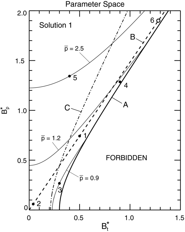
Figure 2. Parameter space for a subclass of non-force-free (NFF) 1D equilibria, Solution 1, in a background plasma of finite pressure pa. Six particular equilibrium configurations are shown by dots "1"–"5" and "6," referred to as solutions S1.1–S1.6, respectively. Thick solid curve A: the equilibrium boundary. Thick dashed line B: all solutions with  . Dash-dot curve C: all solutions with β(0) = 1. Thin solid curves are the constant-
 curves given by Equation (39) for the indicated
  values. Dash-dot curve C intersects the B*t axis at B*t = 0.21213. The solution at this point has
  .
.
Download figure:
Standard image High-resolution imageInequality (40) shows that curve A asymptotes to the straight line
which is shown by dashed line "B" in Figure 2. Equation (37) shows that all the solutions on this line have  . To the left of B they have
  .
.
Equation (38) shows that  defines curves in B*t–B*p space. All constant-
 isocurves asymptote to line B*p = (40/21)1/2Bt* and therefore do not intersect each other. The slope of this line is slightly shallower than that of line B so that all
  isocurves intersect curve A. The minimum value of
  occurs at the intersection of curve A with the B*t axis. Inserting B*p = 0 and B*t = 3/10 in Equation (38), we obtain
  . Thus, for any
  greater than this value, there is a range of possible B*p and B*t for which physical solutions exist. For example, the
  curve crosses A at B*t = 0.57559 and B*p = 0.72882. This family of solutions (S1) cannot describe flux ropes with
  .
.
From time to time, the present NFF solutions will be compared with the Lundquist (1950) solution restricted to x ⩽ 1, which has been widely used to model observed MCs (e.g., Burlaga 1988; Lepping et al. 1990). The untruncated Lundquist solution is given by

where J0 and J1 are the Bessel functions of zeroth and first order, respectively, and λk is the kth zero of J0, i.e., J0(λk) = 0, k = 1, 2, 3, .... The current density for this structure is Jt(x) = λkB0J0(λkx) and Jp(x) = λkB0J1(λkx). This solution is globally FF, i.e.,  for all x. In the usual applications, however, the first zero of J0 is identified, by fiat, as the boundary of the current channel at x = 1, and for x > 0, the field components are taken to be Bt(x) = 0 and Bp(x) = B0J1(λ1)x−1, where λ1 = 2.4048. This gives Jt(x) = Jp(x) = 0 for x > 0. Bessel functions truncated at other zeros of J0 have also been discussed (e.g., Rust & Kumar 1994). The Lundquist solution restricted to any zero of J0 develops a finite jump in the poloidal current jp(x) at x = 1 but no singularities. At x = 1, Jp(x) merely has a finite jump and Bp(x) remains differentiably continuous because J'1(λk) = −λ−1kJ1(λk). Nevertheless, the jump in jp(x) violates the continuity condition, and the Lundquist solution cannot be obtained as a limit of the present solution set. The unrestricted Lundquist solution, having electric current extending to infinity with both components Jt(x) and Jp(x) alternating in signs, is globally FF but is not physical. Note that choosing k > 1 simply means that jt(x) has (k − 1) zeros inside the current channel.
We now examine some representative NFF solutions in detail. They are referred to as S1.1–S1.6 and are shown in Figure 2 by dots "1"–"5" and open circle "6," respectively. Figure 3 shows solution S1.1, specified by B*t = 0.5 and B*p = (350/159)1/2Bt* = 0.741832, which is located on dashed line B. In panels (a) and (b), the solid curves show the components of the field and current, and the dashed curves show B(x) = (B2p + B2t)1/2 scaled to Bt0 = Bt(0) and J(x) = (J2p + J2t)1/2 scaled to Jt0 = Jt(0). Panel (c) shows the radial pressure profile  , exhibiting a small peak inside the current channel. This solution, being on the asymptote given by Equation (41), has
  . The maximum value is
  occurring at x = 0.4121, and the average pressure inside the current channel is
  . As a consistency check, we have also numerically integrated Equation (18) over 0 ⩽ x ⩽ 1 and found the same value. In the present paper, calculated values will be given to the fourth decimal place. Input parameters are given to all decimal places as specified.
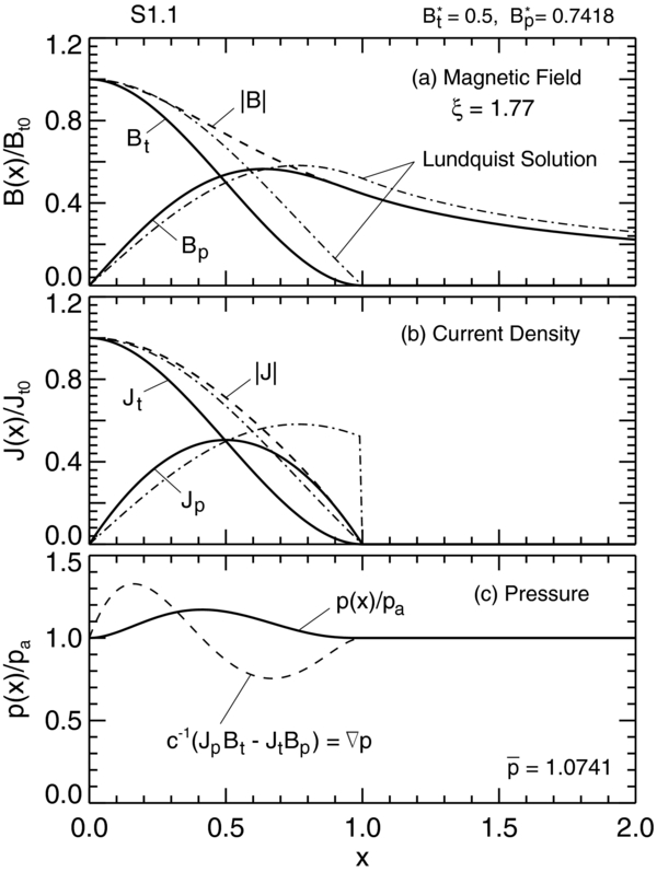
Figure 3. Particular solution S1.1 ("1" in Figure 2) given by B*t = 0.5 and B*p = 0.741832. (a) Bt(x) and Bp(x) are normalized to Bt(0). The dashed curve is B = (B2t + B2p)1/2. The restricted Lundquist solution is shown (dash-dot). (b) Current density components Jt(x) and Jp(x) normalized to Jt(0). The dashed curve is J = |J(x)|. Dash-dot curves: Lundquist solution. (c) Normalized pressure  .
.  and
and  . The Lorentz force FL(x) is overplotted (dashed curve), scaled to fit the plot. FL(0) = FL(1) = 0 is offset to unity.
  .
.
Download figure:
Standard image High-resolution imageIt is convenient to define a parameter
This parameter provides a characteristic measure of the relative magnitude of Bt and Bp. Solution S1.1 has ξ = 1.7690. For fixed value of B*p/Bt*, which defines a line through the origin of the B*t–B*p space (e.g., Figure 2), ξ has the same value for all solutions. Thus, all the solutions on line B have ξ = 1.7690 and the same magnetic field and current profiles.
In panel (c), we have also plotted the dimensionless (radial) Lorentz force (dashed curve) FL(x) defined by Equation (11), which is exactly balanced by the pressure gradient  in equilibrium. In this plot, FL(x) is scaled to fit the plot with FL(0) = FL(1) = 0 offset to unity on the vertical (pressure) axis; only the functional form relative to FL(0) is of significance. This flux rope is Bennet pinch-like in that the poloidal magnetic field confines higher average pressure inside the current channel.
It is useful to measure the overall strength of the forces acting on the flux rope. We define the dimensionless parameter
This quantity satisfies Dp ⩾ 0 and is the volume-averaged magnitude of pressure gradient, which is equal to the Lorentz force, in the current channel. It is straightforward to show that  if and only if
  for all x. This quantity increases as the pressure gradient or equivalently Lorentz force increases. The FF limit corresponds to Dp → 0, so that it can be used to measure the deviation from the FF state. Another useful and equivalent measure of force is
  : Dp = 0 if and only if
  . Solution S1 is characterized by
  . In physical units, the average gradient force is 1.4851 × 10⁻¹(pa/a). This is comparable to
  averaged over the minor radius, where
  .
.
The usual restricted Lundquist solution, Equation (42) applied to x ⩽ 1, is plotted using dash-dot curves in panels (a) and (b). In typical applications (e.g., Burlaga 1988), k = 1 is chosen, meaning that the edge of the current channel is identified with the first zero of J0. The magnetic field profile is similar to that of S1.1 and has ξL = 1.7187, but there is a discontinuity in jp(x) = −dbt/dx at x = 1 (panel b) as discussed above, a qualitative difference from S1.1.
Figure 4 shows the Alfvén speed VA(x) = B(x)/[4πmin(x)]1/2 (solid curve, left axis) scaled to the value on the flux-rope axis VA0 ≡ VA(x = 0) and plasma beta β(x) (dashed curve, right axis), with β = 1 indicated (thin horizontal dashed line). In calculating VA(x), we use mass density ρm = min(x) = mip(x)/2kT, where temperature T is assumed to be uniform in space and mi is the ion mass. Thus, VA(x)/VA0 = B(x)/B(0)[p(0)/p(x)]1/2. For this solution, plasma β at the axis is β0 = 0.3600, remaining less than unity for x ≲ 0.66 and increasing to β(1) = 1.8171 at the edge of the current channel. The average β across the current channel is  . Outside the current channel (1 ⩽ x ⩽ 2), a flux rope typically has β ≫ 1 and is dominated by fluid energy. Accordingly, the Alfvén speed VA(x) is peaked well inside the current channel. This means that if the magnetic field is changed from equilibrium at one end of the system, the resulting changes propagate relatively faster near the axis where the field strength is peaked than outside the current channel. Thus, the core of this flux rope would be better able to maintain its structural integrity.
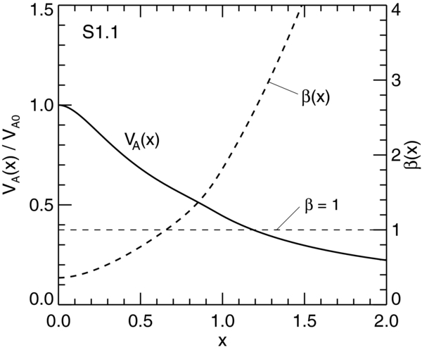
Figure 4. Alfvén speed VA(x) normalized to VA(0) (left axis, solid curve) and plasma β(x) (right axis, dashed curve) for equilibrium S1.1. VA(x) is peaked at x = 0, and β is less than unity for x ≡ r/a ≲ 0.66, indicating structural robustness at the core (x = 0) of the current channel. The outer layer of the current channel with β > 1 is fluid dominated. Equation (16) gives β(0) = βmin = 0.3600 and β(1) = 1.8171 with  . The plasma temperature T is assumed to be uniform in space.
Download figure:
Standard image High-resolution imageShown in Figure 5(a) is the pressure profile p(x) of solution S1.2, given by B*t = 0.04 and B*p = 0.059347 and indicated by "2" in Figure 2. The magnetic field and current density profiles and the value of ξ, being dependent only on B*p/Bt*, are identical to those of solution S1.1 and are not shown. Pressure  , given by Equation (35), does depend on B*p and B*t. Having
  everywhere, this solution is nearly FF. More specifically, it has
  and one maximum
  , with the average pressure
  . The average force magnitude is
  . Compared to the value for S1.1 (
 ), S1.2 is significantly more FF, although the field and current density profiles are identical. Figure 5(b) shows the Alfvén speed (left axis) and plasma β (right axis). As in the case of S1.1, Alfvén speed is peaked at x = 0 and β is minimum inside the current channel. This nearly FF flux rope has β(x) ≫ 1 for all x, having
  and β(0) = βmin = 56.2500.
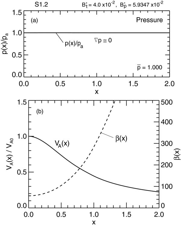
Figure 5. Solution S1.2 ("2" in Figure 2) given by B*t = 4 × 10⁻² and B*p = 5.9347 × 10⁻². The field and current density components are identical in functional forms to those of S1.1 (Figure 3). (a) A nearly force-free solution with |dp(x)/dx| = c−1(JpBt − JtBp) ≃ 0, β ≫ 1 and  . (b) Alfvén speed VA(x)/VA0 (left axis, solid curve) and plasma β(x) (right axis, dashed curve). The self-consistent values are
  and
and  ,
,  , and
, and  . β(0) = βmin = 56.2500.
Download figure:
Standard image High-resolution imageReferring to Figure 2, equilibria in the region bounded by curve A and line B have  . As an example, Figure 6 describes a solution, S1.3, which is denoted by "3" in Figure 2. This point is specified by B*t = 0.3 and B*p = 0.2673. Again, the restricted Lundquist field is shown in panel (a). This solution lies on the
  contour, and we find
  . There is a very small peak,
  , at x = 0.9050. The profile of the Lorentz force for this equilibrium is shown in panel (c) (dashed). For this configuration, Bt is dominant around the axis of the flux rope, and pressure is minimum at x = 0, where β(0) = 0.3606. Overall, however,
  , and β reaches β = 1 at x ≃ 0.32, increasing to β ≃ 14 at x = 1. The β ≪ 1 region is more narrowly localized to the axis of the current channel than for S1.1. Beyond x ≃ 0.3, this flux rope would become increasingly dominated by fluid energy. The average pressure gradient is
  . In this case,
  is somewhat less than the typical gradient because the actual variation in
  occurs within Δx ≃ 0.7. Per the general properties of the S1 family of solutions, bp(x) peaks at x = x* = 0.6376 and jp(x) peaks at x = 1/2. This profile has ξ = 2.9457, significantly different from S1.1.
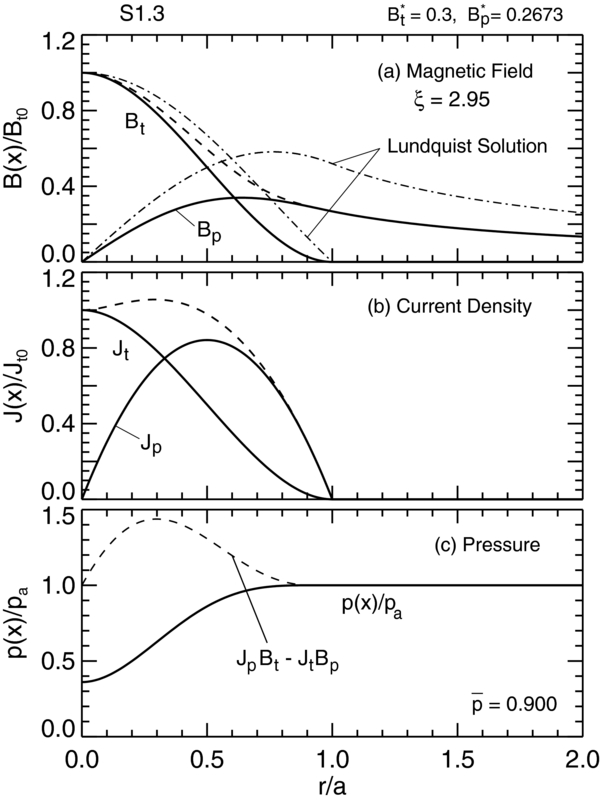
Figure 6. Particular solution S1.3, having  and lying on the
  curve (Figure 2). B*t = 0.3 and B*p = 0.2673. β0 = βmin = 0.3606 and
  . (a) Magnetic field profile is normalized to Bt(0) and is characterized by ξ = 2.9457. (b) Current density distributions, Jt and Jp, normalized to Jt(0). (c) Pressure.
  and
and  . The Lorentz force FL(x) = c−1(JpBt − JtBp) is shown (dashed curve, arbitrary units), with FL(0) = FL(1) = 0 offset to unity.
  .
.
Download figure:
Standard image High-resolution imageFigure 7 shows the pressure profile  for solution S1.4 (labeled "4" in Figure 2) as well as the radial Lorentz force FL(x). This configuration, given by B*t = 0.9 and B*p = 1.2860, is dominated by Bt near the axis with
  at x = 0 and
  at x = 0.5171. Here, we find
  . This is comparable to
  . The average pressure is
  . With ξ = 1.8368, the components of the magnetic field and current density (not shown) are similar to the corresponding quantities of solution S1.1. This flux rope has low β throughout the structure, with β(0) = 3.8637 × 10⁻² and monotonically increasing to unity at x ≃ 1.3. All solutions between curve A and line B have these general characteristics with
  and
and  occurring well inside x = 1. This is an NFF flux rope with β ≪ 1 and has
  . As B*p and B*t are increased, β(0) and
  decrease and
  increases.

Figure 7. Pressure profile of solution S1.4. A highly NFF equilibrium with B*t = 0.9, Bp* = 1.2860 and  . With ξ = 1.8368, the field and current density components are similar to those of S1.1 and S1.2. This solution has
  ,
,  at x = 0.52, and
  . β < 1 throughout 0 ⩽ x ⩽ 1, having β(0) = 3.8637 × 10⁻² increasing to β(1) = 0.6047, with
  . Lorentz force FL(x) (dashed) is scaled to fit the plot with FL(0) = FL(1) = 0 offset to unity.
  .
.
Download figure:
Standard image High-resolution imageShown in Figure 8 is an equilibrium far removed from line B. This solution, S1.5, is characterized by B*t = 0.4 and B*p = 1.34342 and is denoted by "5" in Figure 2. Because this point is to the left of dashed line B with B*p/Bt* ≫ 1, the Lorentz force is dominated by pinch force Jt(x)Bp(x), which is balanced by the significantly higher pressure in the current channel. Specifically, this solution lies on the curve  with the on-axis value of
  as can be calculated using Equation (37). The ratio B*p/Bt* is greater than those of solutions 1–4. Figure 8(a) shows that Bp is dominant for this equilibrium with ξ = 0.7815. As a result, the magnitude of the magnetic field B(x) is peaked away from the axis.

Figure 8. Equilibrium S1.5, given by B*t = 0.4 and B*p = 1.34342.  and
and  for this profile. A highly NFF structure dominated by the poloidal component (highly twisted). (a) Magnetic field components (solid) and magnitude (dashed). ξ = 0.7815. (b) Current density components (solid) and magnitude (dashed). (c) Pressure
  (solid curve). The Lorentz force
  (dashed, arbitrary units scaled to fit the axis) with FL(0) = 0 offset to unity.
  .
.
Download figure:
Standard image High-resolution imageFigure 9 shows the Alfvén speed (left axis, solid curve) and plasma β (right axis, dashed curve) for S1.5. The former has a peak at x = 0.8350, while the latter is highly peaked on the axis with the value β(0) = 4.6868. The minimum of β (βmin = 0.4455) occurs where VA is peaked inside the current channel, and β falls below unity (horizontal dashed line marked β = 1) at about x = 0.5. It remains less than unity to about x ≃ 1.35. The average in the current channel is  . The pronounced peak in β at x = 0 is due to the peak in pressure balanced by pinch force. This structure is much more NFF than the preceding examples and has
  . The fact that VA∝β−1/2 is sharply peaked at x = 0.8350 implies that in a dynamical situation, this flux rope will evolve highly nonuniformly, more rapidly and coherently near the outer edge of the current channel than elsewhere. Where β ≫ 1, the structure is more strongly influenced by fluid dynamics.

Figure 9. Normalized Alfvén speed (solid curve, left axis) and plasma β (dashed curve, right axis) for equilibrium S1.5.  leads to β0 ≫ 1. Equation (16) gives β(0) = 4.6868 and β(1) = 0.5541.
  and βmin = 0.4456 at x = 0.8350.
Download figure:
Standard image High-resolution imageThe parameter space for this family (S1) of solutions has been illustrated using discrete examples. It is straightforward to generalize the understanding to the entire parameter space. Equation (11) shows that B*t (B*p) contributes to the radially outward (inward) Lorentz force and that  and therefore
  scale with B*2t and B*2p. For a given value of B*t, increasing B*p leads to more dominant pinch force, requiring greater average internal pressure to balance the force. Conversely, if B*p is decreased or B*t is increased, magnetic pressure B2t is relatively greater, reducing the required
  and
and  for force balance until the equilibrium limit
  (curve A) is reached. As B*p is increased for given B*t or B*t is decreased for given B*p from dashed line B, the maximum pressure shifts toward the flux-rope axis. Recall that on any given line through the origin, all solutions have identical value of ξ and magnetic field profile, being dependent only on the slope of the line, B*p/Bt*. While the governing parameter is B*p/Bt* for the magnetic field,
  is separately affected by B*t or B*p. For given B*t, the limit of B*p → ∞ yields the Bennet-type pinch. For 0 < B*t < 1/bt(0), the limit B*p → 0 is a solenoidal pinch.
The self-consistent β(x) for the family of solutions can be mapped out in B*t–B*p space. Here, we will consider β(0). Setting β(0) = 1 and substituting Equation (37) in Equation (16) one obtains the thick dash-dot curve labeled C in Figure 2. To the left (right) of curve C, the solutions have β(0) > 1 (β(0) < 1). Solutions S1.1, S1.3, and S1.4 are to the right of curve C, and accordingly have β(0) < 1. Solutions 2 and 5, on the other hand, are to the left of curve C and have β(0) ≫ 1. Setting bt(x = 0) = 10/3 in Equation (16), we find that the β(0) = 1 curve intersects the B*t axis at B*t = (9/200)1/2 = 0.2121. For the solution at this intersection, the average internal pressure is  . Equation (16) shows that β(0) increases with decreasing B*t. Curve C asymptotes to the line given by B*p = (700/159)1/2Bt*.
Because  scales with B*2p and B*2t, one obtains
  as B*p → 0 and B*t → 0. It is illuminating to consider this limit along a line through the origin of the B*t–B*p space (i.e., B*p/Bt* = const). Along such a line, all the solutions have one unique value of ξ and identical magnetic field profiles, but the limit gives
  everywhere and therefore
  . This limit is FF subject to the specified boundary conditions and constraints. This limit also corresponds to
  , as suggested by Equation (16). Figure 5 (S1.2) has provided an example of a nearly FF structure with
  . The limit point itself has B = 0 and as such, is not a magnetic flux rope. As B*p and B*t are increased,
  decreases. Solution S1.6 on line B, given by B*t = 1.280613 and B*p = 1.9 and denoted by "6" (open circle) in Figure 2, is an example of solutions with large B*t and B*p values. For S1.6, β(0) = 5.4880 × 10⁻², increasing to β = 2.7701 × 10⁻¹ at x = 1, and reaching β = 1 at x ≃ 1.9. The β(x) profile of S1.6 is similar to that for S1.1 but is much smaller in value throughout, as indicated by
  . The magnetic field and current profiles (not shown) are identical to those of S1.1 (Figure 3), but the maximum pressure is
  . The average force is
  .
.
To illustrate the above limiting properties, we have computed  and
and  along line B (Figure 2). Figure 10 shows
  (thick solid curve; left axis), β(0) (thin solid curve), and β(1) (dash-dot curve) given by Equation (16), and
  (thick dashed curve; right axis). For these solutions, B*p/Bt* = (350/159)1/2 = 1.4837 and ξ = 1.7690, and the field and current profiles are identical to those of S1.2 (Figures 3 a and 3 b, respectively). It is evident that the limit B*p → 0 leads to
  and
and  , the FF limit. In the opposite limit (B*p → ∞), we find
  (highly NFF) with β(0) → 0 and β(1) → 0. The average β, however, asymptotes to
  , with βmax ≃ 0.1 at x ≃ 0.52. For B*p ≳ 5.0, the solutions yield βmax ≃ 0.1 at x ≃ 0.5 and VA(x)/VA0 ≪ 1 throughout the current channel, with sharp (but continuous) spikes at x = 0 and x ≃ 1. The thickness of the spike decreases with increasing B*p. The pressure profile has
  (e.g.,
  at x = 0.42). Recall that for all of these solutions, p(0) = p(1) = 1, as exemplified by Figure 3.

Figure 10. Limiting properties of Solution 1.  (thick solid), β(0) (thin solid), β(1) (dash-dot), and
  (thick dashed, right axis). The limiting sequence is on line B in Figure 2, satisfying B*p/Bt* = (350/159)1/2. All solutions have ξ = 1.7690. β ≡ 8πpa/〈B2(x)〉 is shown by the thin dotted curve, where 〈⋅⋅⋅〉 means the volume average over the current channel.
Download figure:
Standard image High-resolution imageAlong other lines through the origin, the qualitative properties are unchanged. In particular, for B*p → 0 with a fixed value of B*p/Bt*, one obtains  and
and  . For such lines to the left of dashed line B (i.e., B*p/Bt* > (350/159)1/2), the limit B*p → ∞ may be taken, yielding β(1) → 0 and
  . In contrast,
  asymptotes to a small but nonzero value, while β(0) generally asymptotes to a nonzero value but may vanish as in the present example. Along lines with B*p/Bt* < (350/159)1/2, i.e., those to the right of line B, the limit B*p → ∞ is not physically accessible because of the forbidden region: rather, we find
  , β(0) → 0, and β(1) → 0 as curve A (Figure 2) is approached, where
  and
and  as well as other physical quantities converge to finite values. Because no singularities
  are allowed,
  ,
,  , and other physical quantities are continuous functions of B*p and B*t, as can be inferred from Figure 10. A more extensive parameter study with a wider range of analytic solutions has been tabulated elsewhere (Chen 2012).
3.2. Particular Solution 2
For Solution 1, jp(x) = −dbt(x)/dx is continuous but not smooth at x = 1. We now discuss a distinct family of solutions, henceforth referred to as "Solution 2" or S2 for which we impose djp(x)/dx = 0 at x = 1. To accommodate the added condition, we include an additional term, d4, in bt(x). The general properties (C1)–(C5) discussed at the beginning of Section 3.1 remain unchanged. In particular, the condition  is unaffected, but the value of bt(0) = d0 is modified. Repeating the procedure illustrated in the preceding section and solving the resulting system of algebraic equations for the coefficients, we obtain
Accordingly,
The expressions for bp(x) and jt(x) remain unchanged from Equation (32). For this class of solutions, we have bt(0) = d0 = 5, and bt(x) and bp(x) are independent of B*t and B*p. The existence and the basic structure of the various boundaries and isocurves in B*t–B*p space are unchanged, but the specific curves are determined according to the new form function bt(x).
The self-consistent equilibrium pressure profile is calculated using Equation (14) with Equations (45) and (32). For this solution, the normalized pressure is given by

Because bp(x) is unchanged from that of Solution 1, G(x) is again given by Equation (36), and all the differences are in the expression of bt(x).
As in S1,  and
and  are dependent on B*2p and B*2t separately. For this configuration,
and
One representative solution, designated as S2.1, is shown in Figure 11 in the same format as before. This solution is specified by B*t = 0.4 and B*p = 1.34342, the same parameter values used for solution S1.5 shown in Figure 8. We see that jp(x) smoothly vanishes at x = 1. This requires the peak of jp(x) to be slightly narrower to minimize gradients. As a result, bt(x) is narrower than for S1.5, and bt(x) is maximum at x = 0, monotonically decreasing to the minimum (bt = 0) at x = 1. For this family of solutions, Equation (45) shows that jp(x) increases from zero to the maximum value at x = 1/3 and monotonically decreases to zero at x = 1. Figure 11(c) shows the pressure profile as well as the Lorentz force (normalized, with FL = 0 offset to unity). Equations (48) and (49) give  and
and  . The latter is slightly less than the value for solution S1.5 for which
  . Pressure is peaked off axis with
  at x = 0.0825. This flux rope has
  and
and  . Equations (16) give β(0) = 1.5275 and β(1) = 0.5541. Minimum β = 0.4499 occurs at x = 0.8450, and ξ = 1.1722.

Figure 11. Particular solution S2.1 (Section 3.2). B*t = 0.40 and B*p = 1.34342, the same values as solution S1.5. In addition to the conditions satisfied by Solution 1 (S1.1–S1.6), the requirement dJp(x)/dx = 0 at x = 1 is imposed. For this solution, ξ = 1.1722.  .
.  .
.
Download figure:
Standard image High-resolution imageThe different profile in bt(x) also modifies the equilibrium boundary. Demanding  , we find the equilibrium boundary for this class of solutions:

Compared with Equation (40) for solutions S1, we see that the equilibrium boundary has the same structure except that the numerical coefficient in front of B*2t is larger. This means that the asymptote, B*p = (525/106)1/2Bt*, has a steeper slope than for Solution 1. On this asymptote (the counterpart of line B in Figure 2) all solutions have the same profile and have ξ = 1.7690. The field and current profiles are similar to those of S1.1 and S1.2 except that djp(x)/dx = 0 at x = 1. The boundary curves in B*p–B*t space for S2 are similar to those for S1 (Figure 2). The parameter space map for S2 is given in Chen (2012).
Aside from the differentiability of jp(x) at x = 1, solutions S2 are similar to S1. As in the case of S1, all solutions on a given line through the origin have identical appearance and identical value of ξ. Along each line, B*p → 0 leads to the FF limit  with β → ∞. Other limiting properties can be qualitatively inferred from those of S1.
3.3. Particular Solution 3
For the above two families of solutions, the choice of B*t and B*p determines Bt(x) and Bp(x) and p(x) given pa. The average internal pressure,  , cannot be specified a priori. In reality, a magnetic flux rope may be governed by macroscopic processes that determine B*t,B*p, and
  relative to pa. It is, therefore, desirable to have the ability to separately specify
  . For the third family of solutions, referred to as S3, we specify
  . With this added constraint, we need an additional term in bt(x) or bp(x). Equation (19) shows that the form of bp(x) does not affect
  . We, therefore, increase the number of terms in bt(x) by one by adding d5 ≠ 0 in Equation (45). Imposing the constraints C1–C5 as before, we obtain
with bt(x) = 0 for x > 1. Accordingly,
with jp(x) = 0 for x > 1. Both bp(x) and jt(x) remain the same as in Equations (32) and (34). Thus, G(x) is unchanged from Equation (36). Substituting Equation (51) in equation (14) and averaging over the minor radius, we find
The additional requirement that the average pressure be equal to the specified value  is expressible as
  , which is quadratic in d5. Solving this equation for d5, we obtain
Using  and solving for
  , we obtain
The expression for  is not shown because it is simply a lengthy algebraic expression and provides no significant insight. In the present work, we will use the negative sign in d5.
Unlike S1 and S2, the functional form of bt(x) depends on B*p and B*t through d5, and each value of  determines a sub-family of solutions. This is because by specifying the average pressure,
  , B*t, and B*p become coupled, as can be seen in the expressions for
  . The S3 family of solutions have a relatively high-order term x5 and can exhibit more complex features. While solutions with similar properties and appearance to those of S1 and S2 exist, bt(x) need not be monotonic, which means that jp(x) may reverse signs. For the solutions in this family, p(x) may have a local minimum, which can be negative in the closed interval [0, 1]. Equation (54) further shows that d5 and therefore bt(x) and p(x) may have nonzero imaginary parts. From Equation (54), the condition for real physical quantities is given by

This condition is obviously not affected by the choice of the sign in Equation (54).
We now consider a sub-family of solutions, denoted by S3.0, defined by  . Figure 12 shows a particular solution, S3.01, specified by B*t = 0.34 and B*p = 0.290. Panel (a) shows that bp(x) peaks off axis as does the magnitude B(x) (dashed curve). Panel (b) shows that jp(x) is negative near the flux-rope axis, which is responsible for the reduction in the toroidal component bt(x) near the axis. The magnitude of the current density (dashed curve) is also peaked off the axis. Shown in panel (c) are the pressure
  (solid curve) and the Lorentz force FL(x) (dashed curve, arbitrary units). The self-consistent pressure profile for this solution possesses a minimum
  at x = 0.2275. This configuration is characterized by
  and
and  . For different choices of B*p and B*t,
  may be negative. Thus, the condition
  is only a necessary condition—no longer a necessary and sufficient condition—for physical pressure as discussed below.
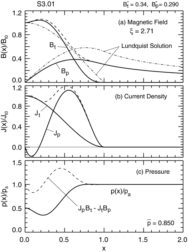
Figure 12. Solution S3.01 given by Equations (51) and (32). The average internal pressure  is specified to be
  . (Bt)max is no longer at x = 0, and Jp(x) is negative near the axis. p(x) can have a minimum inside the current channel. ξ = 2.7110.
  .
.  .
.
Download figure:
Standard image High-resolution imageThe B*t–B*p parameter space for  is shown in Figure 13. Here, the solid curve A is given by the condition
  . All solutions to the left of curve A have
  and are therefore physically inadmissible. As B*t increases away from this curve for given B*p,
  becomes more positive but can acquire a nonzero imaginary part as noted above. The dash-dot curve B in Figure 13 shows the boundary defined by Equation (56). Below curve B, Im(
 ) becomes nonzero, increasing in magnitude with B*t. Solution S3.01 shown in Figure 12 is indicated by "1" in this figure.

Figure 13. Parameter space for sub-family S3.0 of solutions, specified by  . The solution shown in Figure 12 is marked by "1." To the left of the solid curve, the solutions have
  and are forbidden. To the right of the dash-dot curve, the solutions have complex
  and are forbidden. At B*p = 1.00283, there exists one physical solution (open diamond, "a") with
  . Above this value of B*p, all solutions have
  . For B*p ⩽ 0.3350 (open diamond "b"), all solutions have real and non-negative p(x) and physically admissible.
Download figure:
Standard image High-resolution imageThe physically allowed solutions of this sub-family occupy an even smaller part of the space between the two curves. Solution 3.01 in Figure 12 shows a local minimum in  inside the current channel. This dip can become negative as the parameters are varied toward A or B before
  becomes negative or a nonzero imaginary part develops. The restriction becomes more severe as B*t and B*p are increased. Physically, as these parameter values are increased, the value of
  increases, necessitating a decrease in
  to maintain the prescribed average value of
  , ultimately turning
  negative. On the parameter space map, as B*p is increased, physically allowed solutions move away from these two curves. At B*p ≃ 1.002834, there is only one solution with non-negative minimum of
  , given by B*t ≃ 0.7616010 and indicated by the open diamond "a." This solution is not shown but can be easily visualized by taking solution S3.01 and raising the on-axis pressure to
  and lowering the dip to
  . The other differences are that compared to solution S3.01, the dimensional Bp(x) is greater than Bt(x) and Jp(x) is smaller than Jt(x). This configuration has ξ = 1.6983. For B*p > 1.002834, no physically allowed solutions exist. For B*p ⩽ 0.3350, all solutions between A and B are physically acceptable. This value is shown by an open square labeled "b." Thus, S3 is a much more restricted family of solutions than S1 and S2, a consequence of having to satisfy an additional constraint. For the entire S3 family of solutions, the smallest value of
  with real and non-negative pressure is
  , below which no physically admissible solutions are found for any choice of B*p and B*t. The above values of B*p and B*t corresponding to a and b have been determined numerically. For additional solutions for S3, see Chen (2012).
4. FORCE-FREE FLUX ROPES
The FF Lundquist solution has been discussed in Section 3.1.1. Consider now the well-known Gold–Hoyle model (Gold & Hoyle 1960) given by
where Q = const, Bt(x) = B0bt(x), Bp(x) = B0bp(x), and B0 ≡ Bt(0). The parameter Q has a simple geometrical interpretation in terms of the magnetic field pitch Γ(x) given by equation (13). For the above field profile, Γ(x) = Qx. Following a field line at x, one makes ν turns around the axis per unit length of traversal along the toroidal axis. This is expressed as Γ(x) = 2πxaν(x), giving Q = 2πνa. This means ν(x) = Q/2πa = const, i.e., all magnetic field lines have the same number of turns per unit length with no dependence on x.
This magnetic field satisfies Equation (4) with ∇p = 0 for all x. Gold & Hoyle (1960), however, sought to construct an "isolated" flux rope with the field and current restricted to x ⩽ 1. Accordingly, the field was "truncated" at x = 1 with B(x) = 0 for x > 1. This was accomplished by an ad hoc layer of NFF "shielding current" outside the current channel with its thickness determined by an effective resistivity. Here, this resistivity is taken to be zero, and the shielding current layer has zero thickness. The field is piecewise FF—not globally FF—and has a jump in pressure. The singular current layer provides the overall pressure balance at x = 1. The dimensionless current density is
where 1+ ≡ 1 + in the limit of → 0 and J(x) = 0 for all x > 1+. Here, ⩾ 0 is an arbitrarily small number. The normalization is such that J(x) = (c/4π)(B0/a)j(x). The delta functions arise from the discontinuity in magnetic field at x = 1.
Calculating the Lorentz force FL(x) using these components in Equation (11) and integrating Equation (4), one obtains  for x < 1 and
  for x > 1. Thus, it has
  at x = 1. Solving for
  and letting → 0, one obtains

where
Here, bt(1) = (1 + Q2)−1, B*0 ≡ B0/(8πpa)1/2, and  , provided pa ≠ 0. The normalized ambient pressure is
  . Equation (61) shows that
  for all B*0 and Q. The
  requirement leads to

This is analogous to the equilibrium condition (40). This curve is plotted for Q ⩾ 0 in Figure 14 (thick solid curve A). The asymptote of this curve is Q = B*0 (dashed line B). The solutions have  to the left and
  to the right of curve A. On curve A itself, all solutions have
  . On the asymptote B, the value of
  monotonically decreases from the maximum value of
  at B*0 = 0 to
  as B*0, |Q| → ∞. The mirror image of the boundary curves for Q < 0 is not shown, but the sign of Q does not affect the force.

Figure 14. Parameter space of the Gold & Hoyle (1960) equilibria for given pa at r = a. B*0 ≡ B0/(8πpa)1/2. All valid equilibria satisfying Equation (4) must lie above the equilibrium boundary curve A, given by Equation (62). The asymptote to A is shown as dashed line B. The mirror image (Q < 0) is not shown.
Download figure:
Standard image High-resolution imageNote that if the ambient pressure pa can be adjusted to satisfy Equation (61) as may be done in numerical simulations (e.g., Linton et al. 2001), the equilibrium boundary need not arise. It is the requirement that a magnetic field profile satisfy force balance with specified ambient pressure pa that leads to condition (62).
The usual rationale for using the FF simplification in the solar and SW context is that β = 8πp/B2 is so small that pressure force makes negligible contributions to the force balance. Small β, however, means p/B2 → 0, not ∇p → 0, while FF, by definition, means ∇p = c−1 J × B = 0; pressure and therefore β can have any value in a FF structure provided it is spatially uniform. Thus, plasma β is indeterminate for solutions of J × B = 0. Solution S1.2 (Figure 5) is a nearly FF flux rope (∇p = c−1 J × B ≃ 0) with β ≫ 1 while S1.6, with an identical field profile, illustrates a highly NFF ( ) flux rope with β ≪ 1. The FF condition has no bearing on the value of β and vice versa.
With pa ≠ 0, the limit B*p → 0 and B*t → 0 corresponds to solutions with  for all x, which is FF, as discussed earlier. The limit itself, i.e., B*p = 0 and B*t = 0, has | B| = 0 so that it is not a magnetic flux rope, but the solutions in an arbitrarily small neighborhood of the limit have | B| ≠ 0 with arbitrarily large
  and small
  (e.g., Figure 10). Physically, this means that it is not possible to have low-β FF flux ropes (B ≠ 0) satisfying the constraints of no discontinuities and singularities. This limit is distinct from the usual solutions of J × B = 0 without reference to the ambient pressure and boundary conditions. In the present work, dp(x)/dx and B(x) are self-consistently calculated. Indeed, the piecewise FF Gold–Hoyle field discussed here shares the same property as the present solutions: Equation (61) shows that
  if and only if B0 → 0 for fixed Q and therefore β → ∞. Note that the ambient medium may contain a magnetic field arising from a current distribution external to the flux rope (e.g., in the photosphere or below in the solar case). Such a field can certainly affect β of the flux rope (see a laboratory example below), but this does not remove the need to use self-consistent quantities in determining the typical β of the system. In general, a structure is NFF regardless of β values. The usual adage that low-β implies J × B = 0 is misleading.
In the above adage, plasma β in the solar corona is implicitly thought of as the ratio of pa and B'2 where pa is the ambient pressure and B' is the "typical" value of magnetic field of the region of interest. An anonymous referee has suggested that if formulated in terms of the effective β' = 8πpa/B'2, the usual adage might be valid. This approach assumes that B' is a specifiable quantity, but the magnetic field of a structure embedded in a natural plasma medium of given pressure pa is not specifiable. Rather, it is determined by the local force balance, either self-consistently calculated or measured. Accordingly, we have defined β' ≡ 8πpa/〈B2(x)〉, where B(x) is the magnitude of the calculated magnetic field and 〈⋅⋅⋅〉 is the volume average over the current channel. Thus, 〈B2(x)〉 is used to represent the "typical" value. This quantity has been plotted in Figure 10 (thin dotted curve). It diverges as B*p → 0 where  , and for B*p → ∞, β* → 0. The latter behavior differs from that of
  , but overall β' and
  exhibit no significant and qualitative differences with respect to the FF limit. Thus, the usual adage is no more valid in terms of β' than in terms of
  . The question of the specifiability of a proposed parameter in a physical model is a generic issue. The interested reader will find a discussion on specifiability of parameters in physical models in Finn & Chen (1990, Section IIb).
In the present work, the model flux ropes are embedded in a medium with no background magnetic field. The presence of an external applied field would modify the β of equilibrium structures. To include an external field, additional physics must be considered, which is beyond the scope of the work. Nevertheless, the fact that β is not a specifiable quantity and the conclusion that magnetic flux ropes are generally not FF are not altered.
For completeness' sake, the angle η(x) = sin −1(| J × B|/| J|| B|) is plotted in Figure 15 for solutions S1.1/S1.2 (dashed), S1.5 (dotted), S2.1 (dash-dot), and S3.01 (solid). For S1, η(x) → 0 as x → 1 while for S2.1 and S3.01, η(1) does not tend to zero. It is easy to show by substituting x = 1 − into the definition that sin η = −(B*p/Bt*) as → 0 for S1.1 and sin η = −B*p/(Bp*2 + 9B*2t)1/2 as → 0 for S2.1. Similarly, sin η tends to a finite value as → 0 for S3.01. The value and form of η(x) remain unchanged along any straight line through the origin. Quantities such as β, ξ, and η are indeterminate at the origin.

Figure 15. Angle subtended by J(x) and B(x) for solutions S1.1 (dashed), S2.1 (dash-dot), and S3.01 (solid). Solutions S1.1 and S1.2 have the identical η(x) profile because they are on line B (Figure 2) and have the same value of B*p/Bt*. η(1) = 0 for S1, but η(1) ≠ 0 for S2 and S3.
Download figure:
Standard image High-resolution image
It is noted that the Taylor state, which is an approximately constant-α configuration, has low β because it has a strong toroidal field produced by an external rigid metallic coil that can take up the stress exerted by the plasma. In effect, the magnetic field is "rigid." In a natural plasma environment, the boundary conditions are fundamentally different: the magnetic field is generated by plasma currents with the stresses balanced by the local plasma pressure, and β need not be small or uniform throughout the system, as illustrated by Figures 4, 5(b), and 9.
5. DISCUSSION AND SUMMARY
We have presented a class of equilibria for NFF 1D cylindrical flux ropes embedded in a background plasma of pressure pa. This class of flux ropes have the electric current distribution localized to the current channel of radius r = a, and the Lorentz force exerted by the flux rope is balanced by the background plasma pressure alone. The system satisfies Equation (4). The physical constraints are that (1) all physical quantities be continuous and nonsingular, (2) pressure be real and non-negative, smoothly converging to pa, and (3) a flux rope relax to a state of minimum complexity. Mathematically, the minimum complexity condition is expressed as the smallest number of lowest-order terms in the expansions of Bp(x) and Bt(x) using xn. The use of x ≡ r/a assumes that the cross-section has one governing length scale. The equilibrium solutions are characterized by two parameters B*p ≡ Bpa/(8πpa)1/2 and  . The field components Bp(x) and Bt(x) and pressure p(x) are self-consistently calculated. Alfvén speed VA(x) and plasma β(x) inside the current channel are shown to be highly nonuniform, implying that under dynamical conditions, a flux rope would evolve nonuniformly. As a self-organized structure, this nonuniformity in structural robustness is significant. The results are scale-invariant.
The results show that the system admits solutions encompassing the full range of values in the forces and plasma β: 0 < c1| J × B| = |∇p| < ∞ and 0 < β < ∞. Three families of analytic solutions, S1, S2, and S3, have been discussed that satisfy an increasing number of physical constraints: S1 satisfying the constraints listed above (Section 3.1), S2 satisfying an additional differentiability requirement for Jp(x) at x = 1 (Section 3.2), and S3 satisfying the added requirement that the average internal pressure  be equal to a specified value
  (Section 3.3). A novel result is that for each of the families of solutions, the B*t–B*p parameter space has a number of specific boundaries separating regions with distinct types of solutions. In particular, the requirement of real and non-negative pressure leads to boundaries in the parameter space beyond which no physical solution exists. A dimensionless parameter,
  , has been introduced to quantitatively measure the deviation from the FF state,
  . The results show that the FF limit
  corresponds to
  , where
  is the average plasma β in the current channel, while the highly NFF regime,
  , is characterized by
  . This provides a counterexample, based on self-consistent equilibrium solutions, to the prevailing notion that low-β justifies the FF approximation J × B = 0. Where
  is specified, FF solutions generally do not exist.
The main geometrical assumption is that the cross-section of the flux rope is circular with the current limited to within a radius of a. In natural settings, e.g., in the SW, the structure of a flux rope may be subjected to numerous influences that are beyond the simple ones discussed in the present paper. For example, the assumption that the cross-section is circular with one length scale a need not be true. Yet, studies of interplanetary MCs show that such simple magnetic field configurations do capture the basic features of the observed SW structures (e.g., Burlaga 1988). Currently, numerical simulation models (e.g., Riley et al. 2004) are being developed to model more complex flux ropes in the SW.
The present formulation does not exhaust all NFF solutions. For example, the expansion of bp(x) and bt(x) can be formulated differently; it has been noted that bp(x) and bt(x) may be expressed using the lowest even powers of x with only slight differences in the specific solutions. In addition, the minimum complexity hypothesis may be formulated in such a way that the average curvature of the magnetic field is minimized. Such differences are not expected to materially affect the essential physical properties of an NFF flux rope subject to the same physical constraints. As such, the treatment is general and is advantageous where small numbers of constraints are sufficient to characterize the system.
This work was supported by the Naval Research Laboratory Base Program.