


ABSTRACT
The magnetic energy and relative magnetic helicity in two emerging solar active regions, AR 11072 and AR 11158, are studied. They are computed by integrating over time the energy and relative helicity fluxes across the photosphere. The fluxes consist of two components: one from photospheric tangential flows that shear and braid field lines (shear term), the other from normal flows that advect magnetic flux into the corona (emergence term). For these active regions: (1) relative magnetic helicity in the active-region corona is mainly contributed by the shear term, (2) helicity fluxes from the emergence and the shear terms have the same sign, (3) magnetic energy in the corona (including both potential energy and free energy) is mainly contributed by the emergence term, and (4) energy fluxes from the emergence term and the shear term evolved consistently in phase during the entire flux emergence course. We also examine the apparent tangential velocity derived by tracking field-line footpoints using a simple tracking method. It is found that this velocity is more consistent with tangential plasma velocity than with the flux transport velocity, which agrees with the conclusion by Schuck.
Export citation and abstract BibTeX RIS
1. INTRODUCTION
Magnetic energy and helicity in solar active regions are two volume-integrated ideal MHD invariants that describe how energetic and complex an active region is. Computation of these quantities is challenging. Energy estimated from the modeled nonlinear force-free field computed from the observational vector magnetic field on the solar surface, for example, sometimes yields very unrealistic results (DeRosa et al. 2009). One reason is that the boundary data used are from the photosphere, where the field is not force-free (Metcalf et al. 1995). Measurement of vector magnetic field in the chromosphere, where the field is close to force free, is very rare. Another way to estimate magnetic energy is based on the virial theorem (Metcalf et al. 2006). However, it again requires that the vector field on the low boundary be force-free. Estimating magnetic helicity is also difficult. Magnetic helicity in a volume V is defined by  , where B is the magnetic field, and the vector potential A satisfies
  . Thus, estimating helicity requires not only information concerning the magnetic field, but also the vector potential in the volume. Helicity is physically meaningful (gauge invariant) only when no magnetic flux penetrates the surface of the volume V. For active regions in the solar atmosphere, this condition is obviously not satisfied because magnetic flux penetrates the photosphere. For this case, one can use a relative measure of helicity which is "topologically meaningful and gauge-invariant" (Berger & Field 1984). This relative magnetic helicity (for simplicity, hereafter we use magnetic helicity to refer to relative magnetic helicity) in a volume can be defined by subtracting the helicity of the potential field Bp in the volume that has the same vertical field on the photosphere. Computing this quantity has proved to be challenging (Klimchuk & Canfield 1994; Régnier & Canfield 2006). Alternatively, one can integrate over time the energy and helicity fluxes across the solar surface to estimate the energy and helicity stored in an active region. An accurate estimate of the coronal energy and helicity requires that the computation be done from the very beginning of the emergence of the active region.
The magnetic helicity flux across a surface S is expressed by (Berger 1984)

where Ap is the vector potential of the potential field Bp, Bt and Bn denote the tangential and normal magnetic fields, and V⊥t and V⊥n are the tangential and normal components of velocity V⊥, the velocity perpendicular to the magnetic field lines. The integral is done over the surface. When applied to the Sun, it indicates that the magnetic helicity in the corona comes from the twisted magnetic flux tubes emerging from the solar interior into the corona (first term; emergence term hereafter), and is generated by shearing and braiding the field lines by the tangential motions on the solar surface (second term; shear term hereafter; see, e.g., Berger 1984; Kusano et al. 2002; Nindos et al. 2003; Pevtsov et al. 2003; Pariat et al. 2005; Démoulin 2007). If the surface S is planar, then this equation can be rewritten as (Pariat et al. 2005)
where  and
and  represent two photospheric positions and
  is the surface normal pointing into the corona.
Similarly, the magnetic energy (Poynting) flux can be expressed by (Kusano et al. 2002)
Again, the energy flux across the solar surface comes from the emergence of twisted magnetic tubes from the solar interior (first term; emergence term) and is generated by shearing magnetic field lines due to tangential motions on the surface (second term; shear term).
When using Equations (1) and (3) to compute the magnetic helicity and energy in localized volumes of the corona, such as above a computational region in the photosphere, we need to additionally ensure or assume connectivity of the footpoints when the data are only available at the lower boundary, i.e., the photosphere—no field lines should leave through the sides of the localized volume in the corona and return to the surface of the Sun outside of the computational region in the photosphere. The data needed for this calculation are the vector magnetic and velocity fields on the photosphere. Measurements of the vector magnetic field on the photosphere have been made for many years, but, to the best of our knowledge, there are to date no direct measurements of the vector velocity field on the photosphere. Recently, great progress has been made toward inferring the vector velocity field in the photosphere using time-series vector magnetic field measurements (e.g., Kusano et al. 2002; Welsch et al. 2004; Longcope 2004; Georgoulis & LaBonte 2006; Schuck 2008). The input for these algorithms is the time-series vector magnetic field data on the solar surface (usually the photosphere). As the temporal derivatives of the magnetic field are involved in these methods, they require vector magnetic field data with continuous observation, high cadence, and consistency of quality. These requirements limit the use of these models to past observations, because most vector field data with a reasonable cadence were taken by ground-based magnetographs at various observatories where local night and bad weather led to substantial data gaps, and seeing and other conditions further caused inconsistent data quality and produced non-solar motions in the image sequence. Thus, only a few attempts have been made to use these equations to study the energy and helicity buildup in solar active regions using observational data (e.g., Kusano et al. 2002; Nindos et al. 2003; Yamamoto et al. 2005; Yamamoto & Sakurai 2009). For example, Kusano et al. (2002) broke down the helicity flux into the emergence term and the shear term, and studied their contributions to the helicity in the corona in an emerging active region. The data used were a combination of the line-of-sight magnetograms taken by the Michelson Doppler Imager (MDI; Scherrer et al. 1995) and the vector magnetic field data taken by the vector magnetograph at the National Astronomical Observatory of Japan (NAOJ). Yamamoto et al. (2005) and Yamamoto & Sakurai (2009) used the same method to analyze more active regions. Since the vector magnetic field data used in those studies were taken by a ground-based magnetograph, they possess the aforementioned caveats. A test with MHD data further showed that the method they used might not have been sensitive enough to capture the helicity flux (Welsch et al. 2007). Therefore, it is necessary to revisit this topic using better algorithms and better observational data. This is one purpose of this study.
There is another approach proposed to study helicity and energy fluxes across the photosphere. By introducing the flux transport velocity U ( ), Démoulin & Berger (2003) simplified Equations (1) and (3) to
and

They further argued geometrically that the apparent tangential velocity derived by tracking the footpoints of the normal magnetic field is in fact the flux transport velocity (DB03 hypothesis hereafter). This allows the helicity flux to be computed from line-of-sight magnetograms and the aforementioned tracking velocity on the surface. Thus, it suggested a feasible way to study magnetic helicity in active regions because high-quality line-of-sight magnetic field measurements with reasonable cadence have been made available for many years by, for example, the MDI and the Global Oscillation Network Group (GONG). In fact, many studies have been carried out since then (see Démoulin 2007; Démoulin & Pariat 2009 for reviews). For example, using this hypothesis, Zhang et al. (2012) broke down the helicity flux into the shear term and the emergence term, and discussed their contributions to the helicity accumulated in the corona. However, the validity of this hypothesis has been questioned (Schuck 2008; Ravindra et al. 2008). Examining this hypothesis is another purpose of this study.
Specifications of observational data taken by the Helioseismic and Magnetic Imager (HMI; Scherrer et al. 2012; Schou et al. 2012) on board the Solar Dynamics Observatory (SDO; Pesnell et al. 2012), i.e., a full disk field-of-view, continuous observation coverage, and consistent data quality, allow us to study magnetic energy and helicity injection into the active-region corona, especially their buildup and evolution during flux emergence, because full disk measurement provides data that catch the very beginning of the emergence of active regions. In this paper, using HMI vector magnetic field data, we break down the energy and helicity fluxes into the shear term and the emergence term and study the roles they play in energy and helicity buildup in the corona in emerging active regions. Also, we test the DB03 hypothesis with the observational data.
The paper is organized as follow. In Section 2, we briefly describe the HMI instrument, data, helicity flux computation, and the active regions chosen for this study. Analysis and results are presented in Section 3. Our test of the DB03 hypothesis is in Section 4. We conclude this work in Section 5.
2. HMI DATA, HELICITY FLUX, AND TWO EMERGING ACTIVE REGIONS
2.1. Data
We use vector magnetic field data taken by HMI. The HMI instrument is a filtergraph with a full disk coverage at 4096 × 4096 pixels. The spatial resolution is about 1'', with a 0 5 pixel size. The width of the filter profiles is 76 mÅ. The spectral line is the Fe i λ6173 absorption line formed in the photosphere (Norton et al. 2006). There are two CCD cameras in the instrument, the "front camera" and the "side camera." The front camera acquires the filtergrams at six wavelengths along the line Fe i λ6173 in two polarization states with 3.75 s between the images. It takes 45 s to acquire a set of 12 filtergrams. This set of data is used to derive the Dopplergrams and the line-of-sight magnetograms. The side camera is dedicated to measuring the vector magnetic field. It takes 135 s to obtain the filtergrams in six polarization states at six wavelength positions. The Stokes parameters (I, Q, U, V) are computed from those measurements, and are further inverted to retrieve the vector magnetic field. In order to suppress the p-modes and increase the signal-to-noise ratio, the Stokes parameters are usually derived from the filtergrams averaged over a certain time. Currently, the average is done with 720 s measurements. They are then inverted to produce the vector magnetic field using the inversion algorithm Very Fast Inversion of the Stokes Vector (VFISV). VFISV is a Milne–Eddington (ME) based approach developed at High Altitude Observatory (HAO; Borrero et al. 2011). The 180° ambiguity of the azimuth is resolved based on the "minimum energy" algorithm (Metcalf 1994; Metcalf et al. 2006; Leka et al. 2009). With significant improvements in the original algorithm, the disambiguation module for automatic use in the HMI-AIA Joint Science Operations Center (JSOC) is implemented by the NorthWest Research Associates (NWRA) at Boulder. The patches of the active regions are automatically identified and bounded by a feature recognition model (Turmon et al. 2010), and the disambiguated vector magnetic field data of the active regions are deprojected to the heliographic coordinates. Here, we use the Lambert (cylindrical equal area) projection method for the deprojection. For a small area such as a normal active region, the difference in the deprojected maps from different projection methods is very small (R. Bogart 2011, private communication). The vector velocity field in the photosphere is derived from the Differential Affine Velocity Estimator for Vector Magnetograms (DAVE4VM; Schuck 2008) which is applied to the time-series deprojected, registered vector magnetic field data. The window size used in DAVE4VM is 19 pixels, which is selected by examining slope, Pearson linear correlation coefficient, and Spearman rank order between
  and δBn/δt, where Vn and Vt are the normal and tangential velocities, and Bn and Bt are the normal and tangential magnetic fields, as suggested by Schuck (2008). This velocity is further corrected by removing the irrelevant field-aligned plasma flow using
where V⊥ is the velocity perpendicular to the magnetic field line and V is the velocity derived by DAVE4VM. The velocity V⊥ is used to compute energy and helicity fluxes in this paper. Detailed information on HMI vector field data processing can be found in Hoeksema et al. (2012) and Sun et al. (2012).
2.2. Helicity Flux
Two issues are related to the helicity flux: (1) how to compute helicity flux, and (2) how to interpret helicity fluxes that are associated with tangential and vertical flows.
2.2.1. Helicity Flux Computation
The magnetic helicity flux across the photosphere can be calculated from Equation (1) or (2). The integral was done over an area of interest (usually it encloses an active region). The vector potential Ap of the potential field on the photosphere is uniquely determined by the observed photospheric vertical magnetic field and Coulomb gauge by equations (Berger 1997; Berger & Ruzmaikin 2000):

Pariat et al. (2005) showed that the helicity flux density in Equation (1) has spurious signals. Theoretically, these false signals are canceled out completely when the total helicity flux is computed by integrating the flux density over the whole region. However, Pariat et al. (2006) found that the helicity flux computed from Equations (1) and (2) could yield up to a 15% difference, and they attributed it primarily to the fake signals that the flux density produces. They also suggested that the noise in the data makes some contribution. Actually, this difference is caused by the boundary condition chosen to compute the helicity flux density. They used a periodic Green's function via the fast Fourier transform (FFT) to compute the helicity flux via Equation (1) and a free-space Green's function via Equation (2). This difference vanishes completely when the boundary condition on the Green's function is consistently chosen (Liu & Schuck 2012). Given that the actual data set is a remapped cutout of the spherical Sun, it is not clear whether the FFT, free-space Green's function, or finite difference solution with Dirichlet boundary conditions (Schuck 2008) gives a more accurate estimate for the total helicity flux computation. A 15% difference is well within the error from the noise of the vector magnetic field data that is estimated in Section 3.1.1. Therefore, we use the FFT to compute the helicity flux in this paper.
2.2.2. Interpretation of Helicity Fluxes Related to Tangential and Normal Flows
As described in Section 1, the magnetic helicity in the corona comes from the twisted magnetic flux tubes emerging from the solar interior into the corona (the emergence term), and is generated by shearing and braiding of the field lines by the tangential motions on the solar surface (the shear term). The emergence term includes the helicity in the twisted magnetic flux tubes that emerge into the corona and the mutual helicity between the pre-existing magnetic field and this newly emerged field. Similarly, the shear term includes helicity generated by shearing the field lines and the mutual helicity between the shearing field and the background field due to the change of field geometry. Interpretation of the  term that is related to emergence and the
  term that is related to shear motion on the surface was explicitly stated in Berger (1984; see also Kusano et al. 2002; Démoulin & Berger 2003; Nindos et al. 2003; Pevtsov et al. 2003; Pariat et al. 2005; Démoulin 2007).3
2.3. Two Emerging Active Regions: AR 11072 and AR 11158
Two active regions, AR 11072 and AR 11158, are chosen for this study. AR 11072 is a simple active region with a bipolar structure of the magnetic field. It began to emerge on 2010 May 20 at the southern hemisphere (S15E48). No C-class or above flares occurred in this region during its disk passage. AR 11158, on the other hand, is an active region with complex magnetic field configuration. It started to emerge on 2011 February 10 at the southern hemisphere (S20E60), and produced several major flares during its disk passage. Its flare activity and magnetic evolution were described and analyzed in e.g., Sun et al. (2012), Wang et al. (2012), and Jing et al. (2012).
3. RESULTS
3.1. AR 11072
Figure 1 presents snapshots of the normal magnetic field in AR 11072, showing its emergence and evolution. The leading and following fields emerged and moved apart from each other, developing a typical bipolar active region: compact leading polarity (positive) and fragmented following polarity (negative). Figure 2 displays the vector magnetic field at 12:00 UT 2010 May 22. The velocity V⊥ is shown in Figure 3. The tangential velocity (left panel) successfully reproduces the evolutionary characteristics in this region as seen in a magnetic field movie: the leading and following fields separated from each other, and the leading polarity patch appeared to rotate counterclockwise. The normal velocity (right panel) reveals strong upflows at the middle of the active region where the flux emergence took place.

Figure 1. Evolution of the normal magnetic field of AR 11072. White and black in the images refer to the positive and the negative fields. All images are scaled to ±800.0 Mx cm−2.
Download figure:
Standard image High-resolution image
Figure 2. Vector magnetic field of AR 11072 at 12:00 UT 2010 May 22. The active region was at S16W00. The image is the normal field with the positive field in white and the negative in black. It is scaled to ±800.0 Mx cm−2. The arrows represent the tangential field. Blue (red) arrows indicate that the normal fields at those pixels are positive (negative).
Download figure:
Standard image High-resolution image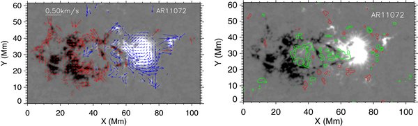
Figure 3. Velocity field V⊥ of AR 11072 at 12:00 UT 2010 May 22. The images are the normal magnetic field saturated at ±800.0 Mx cm−2. The arrows in the left panel refer to tangential velocity, and the contours in the right refer to the normal velocity, with upflows in green and downflows in red. Blue (red) arrows indicate that the normal magnetic fields in the pixels are positive (negative). Only the tangential velocity at the pixels where the normal field is greater than 40.0 Mx cm−2 is plotted. The contour levels are ±0.12, ±0.24, ±0.48 km s−1.
Download figure:
Standard image High-resolution imageEmergence and evolution of the active region are also illustrated in the top panel of Figure 4. The blue, red, and black curves are temporal profiles of positive, negative, and unsigned magnetic fluxes from 2010 May 20 to 26. The unsigned flux is defined to be the summation of the positive flux and the absolute value of the negative flux. We observed that the active region began to emerge at 07:00 UT 21 May, and lasted for 40 hr (from hours 15 to 55). Basically, the magnetic flux in this region was balanced during the course of emergence. The total flux reached 8×10²¹ Mx. The net flux was below 10% of the total unsigned flux in this six-day period. The net flux is the summation of the positive and the negative fluxes. Obviously, any flux imbalance is caused by either limitations in the field of view or measurement limitations and errors. Flux balance is a necessary but insufficient condition for connectivity of the footpoints, and matched footpoints in closed field regions is necessary for an accurate assessment of the Poynting and helicity fluxes through the photosphere into the near corona.

Figure 4. Top: temporal profiles of magnetic flux in AR 11072. Black, blue, and red curves refer to unsigned, positive, and absolute negative fluxes, respectively. The curves start at 16:00 UT 2010 May 20. Middle: temporal profiles of magnetic helicity of AR 11072. Red and blue curves represent helicity fluxes across the photosphere from shear and emergence terms, respectively. 1σ error is presented by the black and green error bars, which are plotted only at several representative times. Violet and light blue curves refer to accumulated helicities in the corona from shear and emergence terms. The black curve is the total accumulated helicity (summation of these two terms). Bottom: temporal profiles of helicity flux across the photosphere from the shear term (red), upflows (blue) and downflows (light blue).
Download figure:
Standard image High-resolution image3.1.1. Magnetic Helicity in AR 11072
Temporal profiles of helicity fluxes across the photosphere are plotted in the middle panel of Figure 4. Red and blue curves represent the helicity fluxes from V⊥t (shear-helicity flux hereafter) and from V⊥n (emergence-helicity flux hereafter), respectively. Recall that V⊥t and V⊥n are the tangential and normal components of V⊥. A 2 hr running average was applied in order to show their average temporal behavior. Violet and light blue curves refer to the accumulated helicities from the shear- and emergence-helicity fluxes, respectively. The accumulated helicity plotted here is the integral of the helicity flux over time, which is deemed to be the helicity stored in the corona. The black curve is the total helicity, i.e., the summation of both terms. Uncertainties in the shear- and emergence-helicity fluxes are also reported by the black and green error bars. They were estimated by conducting a Monte Carlo experiment. In this experiment, we randomly added noise to three components of the vector magnetic field, and repeated the vector velocity and helicity flux computations. The noise added has a Gaussian distribution, and the width (σ) of the Gaussian function is 100 G, which is roughly the noise level of the vector magnetic field (Hoeksema et al. 2012). This test was repeated 200 times. The original error, the root mean square (rms; σ) of these 200 experiments, was then adjusted by the two-hour running average, and finally plotted by error bars in Figure 4. Here, we only plot errors at several representative instants in order to better show the results. Averaging the five original errors of shear-helicity flux between hours 35 and 65, where the shear-helicity flux is significant, yields 23%, which is greater than the maximum difference (15%) of helicity fluxes computed via Equations (1) and (2) and reported in Pariat et al. (2006). The evolutionary characteristics of the fluxes are well above the errors. The shear-helicity flux was dominant. It was high during flux emergence and quickly approached zero after the emergence significantly reduced. Emergence-helicity flux, on the other hand, remained at a very low level for the entire six-day time period. Both helicities were negative. This is in opposition to the so-called hemisphere rule, which predicts that active regions in the southern hemisphere have positive helicity. The total helicity accumulated in the corona in this six-day period was −1.7×1042 Mx2; of this, 88% was contributed by the shear term. We further separated the emergence-helicity flux into two components: helicity flux from upflows (upflow-helicity flux) and from downflows (downflow-helicity flux). Their temporal profiles are shown in the bottom panel of Figure 4, together with the profile of the shear-helicity flux. The upflow- and downflow-helicity fluxes had different signs, while the upflow-helicity flux had the same sign as the shear-helicity flux. Both fluxes were very low. The upflow-helicity flux is from the twisted/sheared field emerging from the interior into the corona and the mutual helicity between this emerging field and the pre-existing field.
To better examine the relationship between magnetic flux emergence and helicity injection, in Figure 5 we plot the temporal profiles of the change rate of the total unsigned flux (black), −1 × shear-helicity flux (red) and −1 × emergence-helicity flux (blue). A four-hour running average was applied. The change rate of the total unsigned flux is normalized by its maximum value, while both helicity fluxes are normalized by the maximum of their summation. There were two quick emergence processes in the early 60 hr period, during hours 10–30 and hours 40–55. The emergence became much less significant thereafter. It also appeared to have a delay between flux emergence and helicity injection, which was reported previously in Tian & Alexander (2008). To determine this delay numerically, we shifted the shear-helicity flux and computed the correlation coefficient between the shifted helicity flux and the rate of change of magnetic flux. The range of the shift is ±20 hr with a step of 0.2 hr. This analysis was applied to the raw data without applying the two-hour running average. A 12.8 hr shift for the shear-helicity flux yields a maximum correlation coefficient, which is 0.32. This infers that there may be a phase lag of 12.8 hr between them. Besides this possible lag, the flux emergence and the shear-helicity flux are well correlated: the shear-helicity flux was significant during emergence, and quickly approached zero after about 70 hr, when the emergence significantly reduced. This indicates that the photospheric shear motion, which produced the most helicity in the corona, was closely related to flux emergence.
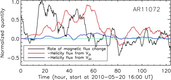
Figure 5. Six-day temporal profiles of the change rate of the photospheric unsigned magnetic flux (black), −1 × (helicity fluxes) from the shear term (red) and from the emergence term (blue), in the active region AR 11072. A four-hour running average is applied to the data. They are normalized by the maximum values of the flux change rate and total helicity flux in this time period, respectively.
Download figure:
Standard image High-resolution image3.1.2. Magnetic Energy in AR 11072
The magnetic energy in AR 11072 was also calculated using Equation (3). The black, blue, and red curves in the top panel of Figure 6 refer to the unsigned, positive, and negative fluxes, respectively. The bottom panel shows the energy fluxes from V⊥t (red; shear-energy flux hereafter) and V⊥n (blue; emergence-energy flux hereafter), respectively. A two-hour running average was applied. Violet and light blue curves refer to integrals of the energy fluxes over time, representing the magnetic energy accumulated in the corona. The black curve is the summation of the two. 1σ errors are plotted at several representative times for shear-energy flux (black) and for emergence-energy flux (green), respectively. Again, they were obtained by conducting a Monte Carlo experiment, the same as for the helicity fluxes. The total energy accumulated in the corona in the six-day period was about 2.8×1032 erg. The emergence-energy flux was dominant, contributing about 61% of the total energy, while the shear-energy flux contributed 39%. Both fluxes had two obvious increases in the first 60 hr, consistent with the timing of flux emergence. This correlation is clearly demonstrated in a phase-relationship plot in Figure 7, where the black curve represents the temporal profile of the change rate of the total unsigned flux, and the red and blue curves refer to the shear- and emergence-energy fluxes, respectively. The two increases coincided with the two significant flux emergence courses: one was from hours 10 to 30, and the other from hours 40 to 55. It also shows that both energy fluxes evolved consistently in phase, but the emergence-energy flux was higher than the shear-energy flux during the entire six-day period. We did a correlation analysis between the energy injection and flux emergence, similar to that between the helicity injection and flux emergence. A three-hour shift of the energy flux yields the maximum correlation coefficient, but it is very small, only 0.15. Another interesting feature in this figure is that after the emergence was significantly reduced, the normal flow still injected significant energy into the corona. This is illustrated by a high emergence-energy flux after hour 60. The source of this energy injection was the upflows that surrounded the leading sunspot, as demonstrated in Figure 8, where V⊥n (left panel) and the emergence-energy flux (right) are overplotted in contours on the normal magnetic field. The data plotted here were taken at 12:00 UT 2010 May 23, after the flux emergence was greatly reduced. Note that although V⊥n showed strong signals in some weak-field areas where magnetic field measurement is less reliable (left panel), the concentrations of the emergence-energy flux are actually in the strong-field areas (right panel). Thus, the strong V⊥n in the weak-field areas contributed much less emergence-energy flux. This is also shown by the small error bar at hour 68 in Figure 6, which was estimated by conducting a Monte Carlo experiment by randomly adding noise to the magnetic field.

Figure 6. Top: same as in the top panel of Figure 4. Bottom: temporal profiles of energy fluxes from the shear term (red) and emergence term (blue). The 1σ errors are shown by the black and green bars. Violet and light blue curves refer to the accumulated energy in the corona from the shear term and the emergence term. The black curve is the sum of the two. The accumulated energy here is the integral of the energy flux over time.
Download figure:
Standard image High-resolution image
Figure 7. Similar to Figure 5, but the red and blue curves refer to the temporal profiles of the energy fluxes from the shear and emergence terms, respectively.
Download figure:
Standard image High-resolution image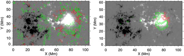
Figure 8. Left: the black-white image is the normal magnetic field of AR 11072 at 12:00 UT 2010 May 23, overplotted in contours by V⊥n. The contour levels are ±0.16, ±0.32, and ±0.64 km s−1, with upflows in green and downflows in red. The image is saturated at ±800 Mx cm−2 with the positive field in white and the negative field in black. Right: the image represents the normal magnetic field, overplotted in contours by the emergence-energy flux density. The green and red contours refer to the positive and negative energy fluxes. The contour levels are ±0.08×10¹⁰, 0.16×10¹⁰, and 0.24×10¹⁰ erg cm−2 s−1.
Download figure:
Standard image High-resolution image3.2. AR 11158
Figure 9 shows the evolution of the normal magnetic field in AR 11158 from 2011 February 12 to 15. It began to quickly emerge on 2011 February 12, and finally developed into a complex, multipolar active region. Figure 10 displays the vector magnetic field at 19:48 UT 2011 February 14. The magnetic field was highly sheared along the polarity inversion line at the middle of the region. The apparently twisted magnetic fields in the negative sunspots were probably caused by the fast spinning of the sunspots. V⊥t (arrows in the left panel of Figure 11) revealed various flow patterns that were consistent with what were shown in the time-series magnetic field data: a separation motion of the leading and following polarities, strong shear motions along the polarity inversion line, and the rotations in the sunspots. Similar to that in AR 11072, the V⊥n map (right panel of Figure 11) exhibits strong upflows surrounding the sunspots. The magnetic flux in this region was well balanced during its emergence, as shown in the top panel of Figure 12.

Figure 9. Evolution of the normal magnetic field of AR 11158 from 2011 February 12 to 15. The images are saturated at ±800 Mx cm−2 with the positive field in white and the negative field in black.
Download figure:
Standard image High-resolution image
Figure 10. Vector magnetic field in AR 11158 at 19:48 UT 2011 February 14 at S20W12. The image represents the normal magnetic field with the positive field in white and the negative field in black. It is scaled to ±800 Mx cm−2. The arrows refer to the tangential field. Blue (red) arrows indicate that the normal fields at those pixels are positive (negative).
Download figure:
Standard image High-resolution image
Figure 11. Same as Figure 3, but for AR 11158. The data were taken at 19:48 UT 2011 February 14, when the region was at S20W12. The images are the normal magnetic field saturated at ±800.0 Mx cm−2. The arrows in the left panel refer to the tangential velocity, and the contours in the right panel refer to the normal velocity with upflows in green and downflows in red. The contour levels are ±0.09, ±0.18, ±0.36 km s−1.
Download figure:
Standard image High-resolution image
Figure 12. Same as in Figure 4, but for AR 11158. The curves start at 00:00 UT 2011 February 12.
Download figure:
Standard image High-resolution image3.2.1. Magnetic Helicity in AR 11158
Temporal profiles of magnetic helicity in this region are plotted in the middle panel of Figure 12. The shear-helicity flux dominated in this five-day period, while the emergence-helicity flux was moderately low. The helicities in the corona injected by both fluxes were positive, which followed the "hemispheric rule." The total helicity accumulated in the corona in this five-day period reached 1.8×1043 Mx2, of which the shear-term contributed about 66% and the emergence-term about 34%. Similar to AR 11072, uncertainties of the shear- and emergence-helicity fluxes were obtained by conducting a Monte Carlo experiment. We also separated the emergence-helicity flux into upflow- and downflow-helicity fluxes. They are plotted in the bottom panel, together with the shear-helicity flux. Upflows and downflows injected helicity of opposite signs into the corona, while the helicity from upflows had the same sign as that from the tangential velocity. The helicity flux from upflows was moderate, but still lower than that from the shear-term.
Figure 13 shows the relationship between the flux emergence and helicity flux. The shear-helicity flux was dominant. Both the shear- and emergence-helicity fluxes were low during the main flux emergence between hours 15 and 40, and the shear-helicity flux significantly increased afterward. A 4.8 hr shift for the shear-helicity flux yielded a maximum correlation coefficient between this flux and the rate of magnetic flux change, but the coefficient was only 0.30.

Figure 13. Same as in Figure 5, but for AR 11158.
Download figure:
Standard image High-resolution image3.2.2. Magnetic Energy in AR 11158
Figure 14 shows temporal profiles of energy fluxes. The uncertainties of shear- and emergence-energy fluxes were obtained by conducting a Monte Carlo test. The emergence-energy flux was again dominant, contributing 62% of the total energy, while the shear-energy flux contributed about 38%. The total energy accumulated in the corona reached 1.3×1033 erg in the five-day period. Both fluxes evolved consistently in phase in the entire flux emergence course, as demonstrated in Figure 15. No phase shift was found between the energy injection and the magnetic flux emergence.

Figure 14. Same as in Figure 6, but for AR 11158. The curves start at 00:00 UT 2011 February 12.
Download figure:
Standard image High-resolution image
Figure 15. Same as in Figure 7, but for AR 11158.
Download figure:
Standard image High-resolution image3.3. Summary and Discussion
We summarize our analysis for the two emerging active regions as follows. Magnetic energy (including both potential energy and free energy) in the corona is contributed mainly by the emergence term. It contributes 61% of the total energy for AR 11072, and 62% for AR 11158. The emergence- and shear-energy fluxes evolve consistently in phase during the entire flux emergence course. Magnetic helicity in the corona, on the other hand, is contributed mainly by the shear term. It contributes 88% of the total helicity for AR 11072, and 66% for AR 11158. Both the shear- and emergence-helicity fluxes have the same sign. If the emergence-helicity flux is separated into the upflow-helicity flux (helicity flux from upflows) and the downflow-helicity flux (helicity flux from downflows), then the upflow-helicity flux was very low in AR 11072 during its entire emergence course, and was low in AR 11158 during its main flux emergence phase during hours 20–50.
As described in Section 1, magnetic helicity in the corona comes from normal flows that advect the twisted magnetic flux into the corona, and is generated by surface flows that shear and braid magnetic fields (e.g., Berger 1984; Kusano et al. 2002; Nindos et al. 2003; Pevtsov et al. 2003; Pariat et al. 2005; Démoulin 2007). With this interpretation, the helicity flux from upflows is deemed to be the helicity that is injected into the corona purely by flux emergence. The result that the shear-term outweighs the upflows in injecting helicity into the corona during the flux emergence suggests a two-stage scenario for the buildup of helicity in the corona: at the beginning, the magnetic field with low helicity emerges into the corona (the first stage); it is then sheared and twisted by surface shearing flows (the second stage), which builds up most of the helicity in the corona. When the field is nonlinear force-free, the relative helicity is found to have "a statistically robust, monotonic correlation" with the free magnetic energy in a sample of 42 active regions (Tziotziou et al. 2012). Thus, the aforementioned scenario implies that the emerged field in these two active regions studied initially contained less free energy. Much more free energy was built up later by the surface shearing flows. The surface flows are probably caused by the flux emergence, which will be discussed in the next paragraph.
Longcope & Welsch (2000) proposed a dynamical model which suggests that only a fraction of the current carried by a twisted flux tube will pass into the corona. This leads to torsional Alfvén waves that propagate along the flux tube, transporting magnetic twist from the highly twisted portion of the flux tube under the photosphere to the less twisted portion of the flux tube that emerges and expands in the corona. This process is manifested in the photosphere with rotational motions of sunspots that are often observed in active regions during their emergence. Pevtsov et al. (2003) tested this model with six emerging active regions. They found reasonable agreement between the model prediction and observation. MHD simulations successfully reproduced the processes that the model predicts (e.g., Magara & Longcope 2003; Fan 2009). More generally, a common feature from simulations of the emergence of a highly twisted flux tube is that it is difficult for the flux tube to rise bodily into the corona entirely. Instead, only the upper parts of the helical field lines of the twisted tube expand into the corona, and this emergence also causes surface flows (e.g., Fan & Gibson 2003; Magara & Longcope 2003; Manchester et al. 2004; Fan 2009; Cheung et al. 2010).
From the helicity-injection point of view, this model predicts that a small amount of helicity is injected by the emergence term due to the emergence of less twisted flux tubes. Much of the helicity is injected by the surface flows that twist and braid the emerged field lines afterward. Thus, the shear-helicity flux is dominant during the flux emergence. Indeed, the MHD simulations from Magara & Longcope (2003) and Fan (2009) have demonstrated that the shear term contributes most of the helicity in the corona during flux emergence. This is consistent with the observational results shown in this study. A significant difference between the MHD simulations and our observational results is that in the MHD simulations, there is a very short impulsive helicity injection from the emergence term at the beginning of the flux emergence, which the observation did not have. The initial twist in the flux tube in these simulations is set to be fairly high. Although the emerged part of the flux tube only has a fraction of the initial twist, it still contains a certain amount of electric current. The emergence of this current-carrying flux tube into the corona certainly injects a great amount of helicity that is reflected in the emergence term, which leads to that short impulsive injection from the emergence term. In the two active regions analyzed here, only low helicity injection, without that impulsive injection, is measured from the emergence term during their emergence. This may indicate that the emerged flux tubes are much less twisted at the beginning. Much of the twist is built up later by the shearing flows.
Another interesting result of this study is that the coronal energy (including both potential energy and free energy) in the active regions is mainly contributed by the emergence term during flux emergence. This agrees partly with what MHD simulations have predicted, that the emergence term contributes substantial energy to the corona (Fan & Gibson 2003; Magara & Longcope 2003; Manchester et al. 2004; Wu et al. 2006; Cheung et al. 2010). However, the MHD simulations predicted that this emergence-term energy injection only takes place in the early phase of flux emergence. In contrast, we found in AR 11072 that this energy injection lasted through the entire course of emergence, and remained fairly high even after the emergence was reduced significantly. The source of this energy injection was the areas surrounding the leading sunspot where strong upflows and tangential magnetic fields are found (see Figures 8).
Breaking down the helicity flux into the emergence term and the shear term in emerging active regions has been studied before, e.g., by Kusano et al. (2002), Yamamoto et al. (2005), Yamamoto & Sakurai (2009), and Zhang et al. (2012). Zhang et al. (2012) made use of the DB03 hypothesis, which is demonstrated in the next section to be incorrect. Kusano et al. (2002) combined the line-of-sight magnetograms taken by MDI and the vector magnetic field data taken by the vector magnetograph at NAOJ to study the magnetic helicity and Poynting fluxes across the photosphere in an emerging active region, AR 8100. They applied a local correlation tracking (LCT) technique to the MDI magnetograms to derive the tangential velocity, and then determined the normal velocity by solving the normal component of the induction equation with the vector magnetic field data and the aforementioned tangential velocity. They found that the photospheric shear motion and the flux emergence process contributed equally to the helicity injection and supplied magnetic helicity of opposite signs into the active region, and the energy flux from the emergence term was dominant in the active region. Using the same method, Yamamoto et al. (2005) and Yamamoto & Sakurai (2009) analyzed more active regions. They found in another emerging active region, AR 8011, that the helicity flux from the shear term first had the sign opposite to that from the emergence term, and later changed sign. The fluxes from both terms were comparable. These results are the opposite of what we found in this study. Besides the limitation on the method they used and the caveats to the data used as mentioned in Section 1, such as outstanding data gaps and the inconsistency of data quality due to seeing and other conditions, there are several other factors that may cause this discrepancy. For example, data from different instruments might need careful cross-calibration, which is not trivial (Leka & Barnes 2012; Liu et al. 2012). The active regions analyzed in their studies and ours are obviously different, and may have different properties during their emergence. Further study is needed.
4. TEST OF THE DB03 HYPOTHESIS
Démoulin & Berger (2003) conjectured that the geometry of the magnetic field in the photosphere implies that the velocity derived by tracking magnetic footpoints (U hereafter) is in fact the flux transport velocity. In this way, the total helicity and energy fluxes across the photosphere can be computed by Equations (4) and (5). This hypothesis has been examined using MHD simulation data (Schuck 2008). The conclusion is reached that "line-of-sight tracking methods capture the shearing motion of magnetic footpoints but are insensitive to flux emergence—the velocities determined from line-of-sight methods are more consistent with tangential plasma velocities than with flux transport velocities." Here, we test this hypothesis using observational data from HMI.
We use a tracking algorithm, the differential affine velocity estimator (DAVE; Schuck 2006), to derive U strictly from the evolution of Bn. The data used are the time-series normal magnetic field for AR 11072 and AR 11158 described in Section 2. The helicity and energy fluxes are then computed using Equations (4) and (5) (DAVE-helicity flux and DAVE-energy flux, hereafter). The DB03 hypothesis predicts that the DAVE-helicity flux should be equal to the summation of the DAVE4VM shear- and emergence-helicity fluxes, and the DAVE-energy flux should be equal to the summation of the DAVE4VM shear- and emergence-energy fluxes. Plotted in the top panels of Figures 16 and 17 are temporal profiles of the shear- (red), emergence- (blue), and DAVE-helicity fluxes (light blue). The black curve represents the total helicity flux, which is the summation of the shear- and emergence-helicity fluxes. The bottom panels are the same as in the top, but for the energy fluxes. The shear- and emergence-helicity and energy fluxes are calculated using the velocity V⊥, i.e., the DAVE4VM-derived velocity with field-aligned plasma flows removed. In both cases, the DAVE-helicity and energy fluxes do not equal the total helicity and energy fluxes estimated from DAVE4VM; admittedly, however, the DAVE-helicity tracks the total helicity fairly well. The DAVE-helicity flux is fairly close to the total helicity flux. It caught about 76% of the total helicity accumulated in the corona in that six-day period for AR 11072, and 83% for AR 11158 in that five-day period. The DAVE-energy flux, on the other hand, is significantly different from the total energy flux. The DAVE-energy flux estimates captured only 3% of the total energy (estimated from DAVE4VM) for AR 11072, and 39% for AR 11158. The combined helicity and energy flux results disagree with the predictions of the DB03 hypothesis.

Figure 16. Top: the shear-helicity flux (red), the emergence-helicity flux (blue), the total of shear- and emergence-helicity fluxes (black), and the DAVE-helicity flux (light blue) for AR 11072. Bottom: same as in the top panel, but for the energy flux.
Download figure:
Standard image High-resolution image
Figure 17. Same as Figure 16, but for AR 11158.
Download figure:
Standard image High-resolution imageWhat is particularly interesting here is that for the DAVE4VM results, the helicity flux is largely determined by the shearing term
whereas for the energy flux, both terms are contributors while the emerging term dominates:
Noting that V⊥n is non-zero over much of the active region, Equation (8) implies that  . Figure 18 shows the distribution of the angle between Ap and Bt. On the left is a histogram of the angle for AR 11072, using the vector magnetic field data taken at 12:00 UT 2010 May 22. On the right is the same for AR 11158 at 19:48 UT 2011 February 14. Only pixels with a tangential field greater than 100 G, roughly the noise level of the HMI vector field data (Hoeksema et al. 2012), are counted here. The median of the angle is 95° for AR 11072, and 75° for AR 11158. In both cases, the peaks of the distributions are close to 90°, implying
  .
.

Figure 18. Distribution of the angle between Ap and Bt. Left: histogram of the angle for AR 11072. The angle is computed using the vector magnetic field data taken at 12:00 UT 2010 May 22. Right: histogram of the angle for AR 11158. The data used were taken at 19:48 UT 2011 February 14. Only pixels with Bt greater than 100 G are counted.
Download figure:
Standard image High-resolution imageAs another test, we directly used the total vector velocity derived by DAVE4VM, without removing the field-aligned plasma flows, to calculate the individual energy- and helicity-flux terms (this is technically incorrect for computing the individual terms). Plotted in the top panels of Figures 19 and 20 are temporal profiles of the Vt-term (red),Vn-term (blue), and DAVE-helicity fluxes (light blue). The black curve represents the total helicity flux, which is summation of the Vt-term and Vn-term helicity fluxes. The bottom panels are the same as in the top, but for energy fluxes. Vt and Vn are the tangential and normal components of velocity derived by DAVE4VM. Again, in both cases, the DAVE-helicity and energy fluxes do not equal the total helicity and energy fluxes (which are identical to the total fluxes in Figures 16 and 17). Instead, the DAVE-helicity and energy fluxes agree very well with the Vt-term helicity and energy fluxes. To be more quantitative, in another test, we calculated Pearson linear correlation coefficients between Vt and U(DAVE), and between U(DAVE4VM) and U(DAVE) for each active region. Here, U(DAVE) denotes the tangential velocity inferred by DAVE, and U(DAVE4VM) is the flux transport velocity computed by  , where
  and V⊥n are the tangential and normal components of velocity V⊥, derived by DAVE4VM with the field-aligned plasma flows removed.
  and Bn are the tangential and normal fields. We also calculated the vector correlation coefficient and the Cauchy–Schwarz inequality (Schrijver et al. 2006). The vector correlation coefficient is defined as
where Vi and Ui are the velocities at pixel i. The Cauchy–Schwarz inequality is defined as
where M is the total number of pixels in the region studied. Here, we only use two components of the vector velocity field, i.e., the tangential velocity, to compute Cvec and Ccs. The data used were taken at 12:00 UT 2010 May 22 for AR 11072, and at 19:48 UT 2011 February 14 for AR 11158. Only the pixels with the tangential and normal fields greater than 100 G were selected for those computations. The result is shown in Table 1, where CC refers to the Pearson linear correlation coefficient, Cvec denotes the vector correlation coefficient defined by Equation (10), and Ccs is the Cauchy–Schwarz inequality defined by Equation (11). It is shown that the coefficients between the  and
and  (DAVE) are much higher than those between
  (DAVE4VM) and
  (DAVE) in all measures. These further confirm the conclusion in Schuck (2008) that the velocities determined from tracking methods are more consistent with tangential plasma velocities than with flux transport velocities. These tangential plasma velocities contain the field-aligned plasma flows. Without vector magnetic field data, these flows cannot be removed to accurately compute the individual shearing and emergence contributions. Thus, the line-of-sight magnetograms cannot even be used to calculate the shear term reliably.

Figure 19. Top: Vt-term helicity flux (red), Vn-term helicity flux (blue), total of Vt-term and Vn-term helicity fluxes (black), and DAVE-helicity flux (light blue) for AR 11072. Bottom: same as in the top panel, but for the energy flux.
Download figure:
Standard image High-resolution image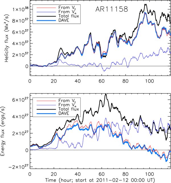
Figure 20. Same as Figure 19, but for AR11158.
Download figure:
Standard image High-resolution image
Table 1. Comparison of Different Velocities
| Active Region | Comparison | CC [Vx] | CC [Vy] | Cvec | Ccs |
|---|---|---|---|---|---|
| AR11072 |  vs. vs.  (DAVE) (DAVE) |
0.98 | 0.96 | 0.97 | 0.95 |
| AR11072 |  (DAVE4VM) vs. (DAVE4VM) vs.  (DAVE) (DAVE) |
0.78 | 0.77 | 0.79 | 0.87 |
| AR11158 |  vs. vs.  (DAVE) (DAVE) |
0.98 | 0.98 | 0.98 | 0.95 |
| AR11158 |  (DAVE4VM) vs. (DAVE4VM) vs.  (DAVE) (DAVE) |
0.76 | 0.70 | 0.73 | 0.81 |
Notes.  and
and  in the second column denote the tangential and normal velocities derived by DAVE4VM.
  (DAVE) is the tangential velocity derived by DAVE.
  (DAVE4VM) is the flux transport velocity computed by
  , where
  and V⊥n are the tangential and the normal components of velocity V⊥, derived by DAVE4VM with the field-aligned plasma flows removed.
  and Bn are the tangential and normal fields. CC represents the Pearson linear correlation coefficients between different velocities in the x-axis (third column) and the y-axis (fourth column). Cvec and Ccs in columns 5 and 6 refer to the vector correlation coefficient and the Cauchy–Schwarz inequality, respectively.
Download table as: ASCIITypeset image
5. CONCLUSIONS
Using HMI vector magnetic field data, we study magnetic helicity and energy in the corona in two emerging active regions, AR 11072 and AR 11158. The magnetic helicity and energy in the corona are calculated by integrating over time the helicity and energy fluxes across the photosphere. These fluxes consist of two components. One is from the photospheric shear motion (shear term), and the other from emergence (emergence term). The vector velocity field on the photosphere is derived by applying DAVE4VM to the time-series vector magnetic field data, and is further corrected by removing the irrelevant field-aligned plasma flow. It is found that the magnetic energy (including both the potential energy and free energy) in the corona is contributed mainly by the emergence term: for AR 11072, the emergence term contributes 61% of the total energy; for AR 11158, it is 62%. During the entire emergence course, the emergence-energy flux is higher than the shear-energy flux, and both fluxes evolve consistently in phase. In AR 11072, the emergence-energy flux remains fairly high after the flux emergence becomes much less significant. The source of this energy injection is the areas surrounding the leading sunspot, where strong upflows and the tangential magnetic field are observed.
Magnetic helicity in the corona is mainly contributed by the shear term. For AR 11072, it contributes about 88% of the total helicity; for AR 11158, it is 66%. Both the shear- and emergence-helicity fluxes have the same sign. The helicity flux from upflows is very low in AR 11072 during its entire emergence, and low in AR 11158 during its main flux emergence phase. This implies that the emerged field initially contained low helicity. Much more helicity was built up afterward by the photospheric shearing flows that twisted and braided the field lines, which is supported by the result that the shear term contributes most of the helicity in the corona. When the magnetic field is force-free, it is found that there is a monotonic correlation between the magnetic helicity and free energy (Tziotziou et al. 2012). Thus, the aforementioned results imply that the free magnetic energy is initially low in the emerged magnetic field, and much of the free energy is built up later by the shearing flows.
Using HMI data, we also examine Démoulin & Berger's (2003) hypothesis. The test shows that the helicity and energy fluxes calculated from the apparent tangential velocity derived by tracking the footpoints of the magnetic field are consistent with those from the tangential plasma velocity, but do not equal the total fluxes as predicted by the hypothesis. This further confirms the conclusion in Schuck (2008) that the velocities determined from simple tracking methods such as LCT and DAVE are more consistent with tangential plasma velocities than with flux transport velocities. In the two emerging active regions studied here, the helicity in the corona was mainly contributed by the tangential flows. Therefore, the helicity computed from the tracking velocity is considered to be a fairly good approximation of the total helicity. The energy is significantly different, however.
We thank the team members who have made great contributions to this SDO mission for their hard work. We also thank the anonymous referees for their critical comments which helped improve the paper. This work was supported by NASA Contract NAS5-02139 (HMI) to Stanford University. The data have been used courtesy of NASA/SDO and the HMI science team.