


ABSTRACT
This paper presents the first potential connections made between two local features in velocity space found in a survey of M giant stars and stellar spatial inhomogeneities on global scales. Comparison to cosmological, chemodynamical stellar halo models confirms that the M giant population is particularly sensitive to rare, recent and massive accretion events. These events can give rise to locally observed velocity sequences—each made from a small fraction of debris from a massive progenitor, passing at high velocity through the survey volume, near the pericenter of the eccentric orbit of the system. The majority of the debris is found in much larger structures, whose morphologies are more cloud-like than stream-like and which lie at the orbital apocenters. Adopting this interpretation, the full-space motions represented by the observed M giant velocity features are derived under the assumption that the members within each sequence share a common space velocity. Orbit integrations are then used to trace the past and future trajectories of these stars across the sky revealing plausible associations with large, previously discovered, cloud-like structures. The connections made between nearby velocity structures and these distant clouds represent preliminary steps toward developing coherent maps of such giant debris systems. These maps promise to provide new insights into the origin of debris clouds, new probes of Galactic history and structure, and new constraints on the high-velocity tails of the local dark matter distribution that are essential for interpreting direct dark matter particle detection experiments.
Export citation and abstract BibTeX RIS
1. INTRODUCTION
There is a long history of using individual stars to map Galactic structure. Studies have gradually evolved from understanding the gross structure of the Galaxy and our place within it (e.g., Herschel 1817; Kapteyn 1922; Shapley 1928), to clarifying the number and character of major structural components—for example, debating the existence of distinct thin and thick disk components (see, e.g., Gilmore et al. 1989; Majewski 1993; Bovy et al. 2012) and the nature and shape of the Galactic bulge (e.g., Weinberg 1992), with its putative X-like structure (McWilliam & Zoccali 2010; Saito et al. 2011) and perhaps multiple bars (Nishiyama et al. 2005). The last two decades have seen vast increases in the sizes of stellar photometric catalogs, which have allowed this field to grow to include the study of substructure within the Galaxy. Stars selected from large-scale photometric surveys have revealed a wealth of spatially coherent overdensities in the stellar halo beyond the disk of our Galaxy—for example using the Sloan Digital Sky Survey (SDSS; Newberg et al. 2002; Belokurov et al. 2006a) and the Two Micron All Sky Survey (2MASS; Majewski et al. 2003; Rocha-Pinto et al. 2003, 2004, 2006). The substructure is dominated by the tidal streams from the ongoing destruction of the Sagittarius dwarf galaxy, which arc dramatically over the Galactic poles (Ibata et al. 2001; Majewski et al. 2003; Belokurov et al. 2006a). There are also numerous smaller streams from both long-dead satellites (e.g., the Orphan Stream— Belokurov et al. 2006a) and globular clusters (e.g., Odenkirchen et al. 2003; Grillmair & Johnson 2006). Less-well studied, but also ubiquitous in these photometric surveys are amorphous clouds of debris—the most prominent being the Triangulum–Andromeda and the Hercules-Aquila Clouds (TriAnd and HerAq; see Majewski et al. 2004; Rocha-Pinto et al. 2004; Belokurov et al. 2007) and the Virgo and Pisces Overdensities (VOD and POD; see Jurić et al. 2008; Sharma et al. 2010).
Substructure has also been found in other dimensions—indeed VOD and POD were seen as groupings in velocity space along limited lines of sight (Newberg et al. 2002; Watkins et al. 2009; Kollmeier et al. 2009) before their full extent was subsequently revealed with photometric maps. The discovery of similar moving groups in the disk (e.g., Eggen 1977) predates the modern studies (see summary in Majewski et al. 1994), and the origin of these disk substructures has been interpreted as either relic associations from their common birth places in ancestral star clusters or due to stars trapped in resonances with disk and spiral arms (Dehnen 2000; Bovy & Hogg 2010). In the halo, moving groups are thought to be the signature of the disruption of accreted objects. Such associations have been found locally in full-space motions (e.g., Eggen & Sandage 1959; Majewski et al. 1994, 1996; Helmi et al. 1999; Kepley et al. 2007; Morrison et al. 2009) and on larger scales using line-of-sight velocities alone (e.g., Ibata et al. 1995; Newberg et al. 2002; Klement et al. 2009; Schlaufman et al. 2009; Williams et al. 2011). In many cases, the significance of tentative associations has been bolstered by similarities in the chemical abundances of member stars (e.g., Majewski et al. 1996; Chou et al. 2007, 2011), or clear stellar-population sequences in color–magnitude diagrams (e.g., Williams et al. 2011).
This plethora of discoveries has inspired concurrent theoretical work to combine our understanding of debris dynamics, hierarchical structure formation, and the evolution of stellar populations. This combination allows us to use observations of substructures around the Milky Way in a variety of ways.5
- 1.
- 2.Confirming our expectations for the level of substructure from hierarchical models of structure formation (Bullock et al. 2001; Bullock & Johnston 2005; Cooper et al. 2010; Rashkov et al. 2012) in space (Bell et al. 2008; Sharma et al. 2010), velocities (Harding et al. 2001; Xue et al. 2011; Helmi et al. 2011), and stellar populations (Font et al. 2006, 2008; Bell et al. 2010).
- 3.
- 4.
This paper builds on the understanding of stellar halo substructure developed over the last two decades, bringing together the underlying themes of discovery, connection, and interpretation. This work is inspired by the combined implications of three distinct studies. The first study explores the morphologies and origin of substructure in a model of a stellar halo built by superposing simulations of individual accretion events (Bullock & Johnston 2005). Debris structures with both stream-like and cloud-like morphologies are apparent. In some cases, there are two or even three distinct clouds associated with a single disruption event—the analogs of "shells" seen around other galaxies (Malin & Carter 1983; Quinn 1984) but viewed from an internal rather than external perspective. The clouds represent debris slowly turning around at the apocenters of orbits that are typically more eccentric than those of the debris streams (Johnston et al. 2008). The implication of this work is that there must be low-density stellar streams moving between these apocentric clouds and passing through the inner Galaxy at high speed near the pericenters of these eccentric orbits—we will hereafter refer to streams of this type as a pericentric streams to distinguish them from tidal streams that are apparent in spatial maps at much higher density.
In the second study, Sharma et al. (2010) apply a group finder to an M giant catalog derived from 2MASS covering large scales (10 < Ks, corresponding to distances d in the range ∼10–100 kpc). The group finder recovers many of the already known substructures, including Sagittarius, provides the first spatial map of POD that revealed its cloud-like morphology, and identifies several other amorphous overdensities, whose nature has yet to be confirmed.
The third study (Sheffield et al. 2012, hereafter referred to as Paper I) is a survey of 1799 line-of-sight velocities (radial velocities, RVs) of relatively nearby (Ks < 9, with distances within ∼10 kpc), moderate Galactic latitude (30° < |b| < 60°) M giant stars selected from the 2MASS catalog. As anticipated, the survey is dominated by thick disk stars, but also shows suggestive velocity–longitude sequences in a smaller population of "RV outliers" (i.e., those with high velocities relative to the Sun). Follow-up high-resolution spectroscopy of samples of these RV outliers reveals that many have abundance patterns consistent with an accreted population and inconsistent with one formed in situ early on in the Galactic halo or disk; this common chemistry lends some support to the proposal of a real physical association between stars in the suggestive sequences.
In this paper, we look at an intriguing question raised by these studies: whether the sequences of M giant RV outliers identified in the inner Galaxy in Paper I actually represent pericentric streams between the apocentric clouds of M giants identified in the outer Galaxy by the group finder in Sharma et al. (2010). While neither the inner-Galactic velocity sequences nor the outer-Galactic spatial overdensities may be entirely convincing as real physical associations in themselves, exploring possible connections between the two at least allows us to make predictions of observable properties these tentative structures must fulfill if they are related, and these predictions can be tested with future surveys.
Any successful attempt at making these connections—from pericentric streams to apocentric clouds or even from clouds to clouds—could have far broader implications. In both observations and models of stellar halos, debris clouds occur with a similar frequency to streams, yet the former have received far less attention. The proposed connections would provide the first comprehensive maps of systems creating cloud-like debris. Indeed, they would be among the first maps of any debris system to explore the full range of orbital phases, from pericenter to apocenter: of all the substructures around our Galaxy, only the streams from Sgr have been followed for more than one radial orbit. The great extent of Sgr's debris has allowed a particularly detailed view of its history, as well as constraints on the depth and triaxiality of the Milky Way's potential (e.g., Johnston et al. 1999a, 2005; Ibata et al. 2001; Helmi 2004; Law et al. 2009; Law & Majewski 2010). Extensive maps of debris clouds could provide similar constraints on their individual histories, on the Galaxy's accretion history and on the Galaxy's mass distribution. Moreover, conclusive evidence for, and measurements of, the velocity of streams of stellar debris passing at high speed through the solar vicinity between these clouds could be used to help predict and interpret signatures of the associated dark matter in direct detection experiments, contributing to what we can say about the nature of dark matter (see, e.g., Kuhlen et al. 2012).
In Section 2, we review the observational and model data utilized in the paper. In Section 3, we "observe" our model stellar halos to understand the strengths and limitations of our observational survey, and develop and test our interpretation methods. In Section 4, we apply the methods developed in Section 3 to the stellar sequences in our survey and compare our predictions to observed data sets. We summarize our conclusion in Section 5.
2. DATA SETS
2.1. The M Giant Survey
The M giant survey described in Paper I has two goals: (1) to study the bulk characteristics of the thick disk and (2) to study the nearby halo, in particular the accreted component. Following Majewski et al. (2003), M giant candidates were selected from the 2MASS on the basis of their color: 96% have (J − Ks)0 > 0.85. To isolate mainly thick disk and nearby halo stars, cuts in Galactic latitude of 30° < |b| < 60° and apparent magnitude were imposed. The range in KS, 0 spans 4.3 <KS, 0 <12.0, with a mean of 7.5 and a standard deviation of 1.3. Spectra of the candidates were taken using the medium-resolution FOBOS spectrograph on the 1 m telescope at the Fan Mountain Observatory (Crane et al. 2005) and the Cassegrain spectrograph on the 1.5 m telescope at Cerro Tololo Inter-American Observatory and the results for the first 1799 stars are presented in Paper I. The RVs have an estimated error of 5–10 km s−1, based on repeat observations and also on comparisons with follow-up high-resolution spectra.
Figure 1 summarizes the data by plotting the line-of-sight velocity (RV) in the Galactic standard of rest (vGSR) frame as a function of Galactic longitude l. The velocities are divided by cos (b) (where b is Galactic latitude) to project disk stars moving at similar velocities in the disk plane into a tighter distribution. Many RV outliers are apparent outside the disk distribution, some making suggestive sequences in this plane. Follow-up, high-resolution spectroscopy of 34 of these RV outliers in Paper I showed that many had abundance patterns consistent with a recently accreted population with low metallicity and α-element abundances reminiscent of those seen in surviving Milky Way satellite galaxies. The abundance results lend some support to the interpretation of the sequences as the signature of real physical associations related to satellite accretion and motivate the work in this paper. The high-resolution spectra also enable a more accurate estimate for the distances of these stars because the improvement in the measurement of the spectroscopic line widths allows a better determination of both metallicities and surface gravity. Two particular sequences (referred to as Groups D and E) that are analyzed in detail in this paper are highlighted in black in the lower panel of Figure 1, with those with high-resolution spectra outlined by circles.

Figure 1. Radial velocity distribution of our M giant survey. Both panels show the line-of-sight velocities projected to the disk plane by a cos b normalization, in the Galactic longitude range −20° < l < 160°. The black symbols in the lower panel correspond to stars selected to be part of the two groups chosen for detailed study here. Those points enclosed in circles represent stars having high-resolution spectra and abundance measurements.
Download figure:
Standard image High-resolution image2.2. The Simulated Survey
We compare the M giant data to the 11 stellar halo models described in Bullock & Johnston (2005). The models were built entirely from accretion events drawn from histories representing random realizations of the formation of a Milky Way type galaxy in a ΛCDM universe. Each accretion event was followed with an individual N-body simulation of a dwarf galaxy disrupting around a host galaxy represented by an analytical potential whose properties smoothly evolved to reflect the full accretion history. The particles in each of these simulated dwarf galaxies had equal dark matter masses and were given (varying) associated stellar masses in such a way that the luminous material reproduced the structural scaling relations observed for Local Group dwarfs (e.g., Mateo 1998). Star formation histories were assigned to the star particles within each accreted dwarf using a simple leaky-accreting-box model of star formation and chemical enrichment that was abruptly truncated upon accretion (Robertson et al. 2005; Font et al. 2006). Once all of the simulations had been run, the phase-space structure of the full stellar halo was constructed by superposing the final positions and velocities of particles from all the individual accretion events contributing to the parent galaxy.
We created simulated surveys of our model halos using the Galaxia code (Sharma et al. 2011a), which can generate a mock observational survey from a given N-body model. The code takes the star formation and chemical evolution histories of the satellites in the models and uses Padova isochrones (Bertelli et al. 1994; Girardi et al. 2000; Marigo & Girardi 2007; Marigo et al. 2008), to generate the observable properties of these stellar populations. A mock M giant survey was created by applying the same cuts to the models as to the 2MASS catalog in Paper I, namely, selecting stars: in the latitude range 30° < |b| < 60°, with (J − Ks) > 0.85 and 0.22 < (J − H) − 0.561(J − Ks) < 0.36, and apparent magnitudes Ks < 9.
We caution that our simulated surveys are not expected to provide accurate predictions of the structure of stellar halos in local volumes around the Sun for several reasons: (1) there is no component of stars formed either in situ in the main halo or kicked out from the Galactic disk, both of which could be a significant contributor in this region (see Abadi et al. 2006; Zolotov et al. 2009, 2010; Purcell et al. 2010; Font et al. 2011; Tissera et al. 2012, for discussions of these formation mechanisms for halo stars); (2) the parent galaxy is represented by analytical functions in the N-body simulations, so there is no mixing of stars due to violent relaxation during significant mergers; (3) the models were constructed before the discovery of the ultrafaint satellites (e.g., Willman et al. 2005; Belokurov et al. 2006b), so they only contain contributions from more luminous satellites; and (4) due to limited numerical resolution of the N-body models, Galaxia has to oversample the N-body particles when generating stars. The oversampled stars need to be dispersed in phase space, which degrades the sharpness of velocity structures (in the generated mock data the ratio of the number of stars to the number of N-body particles is about 2).
Nevertheless, while a direct comparison of (say) the ubiquity or mass spectrum of substructure in the data and the models is not relevant to our goals here, these models are useful for developing some intuition on the meaning of our observational results. In particular, in Section 3 we use them to illustrate how our selection of stellar populations could change our view of the local halo: e.g., what specific substructures in our data might represent and what these substructures could be telling us about the formation and global structure of the stellar halo. We then use this understanding in Section 4 to interpret the nature of the observed M giant structures.
3. RESULTS I: EXAMINATION OF THE SYNTHETIC SURVEYS
The left-hand panel of Figure 2 shows three examples of our simulated surveys projected onto the same plane as the observations in Figure 1. Note that there is no disk component in our synthetic surveys, and only 1 in 10 of our simulated M giants are displayed to mimic the approximate number of RV outliers present in the data taken in the real survey. All panels illustrate the general result of these surveys: stars are mostly distributed randomly in the plane, but with some distinct groups and sequences across spans of tens of degrees in Galactic longitude l. In particular, the top and bottom panels contain examples of distinct linear sequences (highlighted in red and purple, respectively, in the right-hand panels, hereafter referred to as Groups 1 and 2 and described more fully below), reminiscent of the structure of some of the groups selected from the M giant observations. Moreover, like the observed groups, these simulated groups have abundances distinct from the bulk of the stellar halo from which they are drawn: 72% of the stars in Group 1 and 53% in Group 2 have [α/Fe] <0.1, while their parent stellar halo populations both have 30% of their populations with [α/Fe] <0.1.

Figure 2. Same as Figure 1 but for our synthetic surveys M giants for three example simulated halos (left-hand panels). Only 1 in 10 of the synthetic M giants were plotted to show a number of RV outliers comparable to those seen in Figure 1. In the right-hand panels, only particles from satellites contributing more than 10% of the stars to each synthetic survey are plotted, color coded by satellite progenitor. Note the prominent velocity sequences features in red in the top panel ("Group 1") and purple in the bottom panel ("Group 2").
Download figure:
Standard image High-resolution image3.1. Biases Inherent in our Group Selections
Before looking more closely at the properties of the Groups 1 and 2 in our synthetic surveys, it is useful to consider how the nature of the survey itself could bias our view of the stellar halo. M giants are relatively rare in the stellar halo because their progenitors have to be fairly metal rich to evolve into such late type stars. This is in part why debris from the relatively metal-rich Sagittarius dwarf galaxy is so obvious in M giants—this tracer in particular enhances the contrast of Sgr members against the (generally more metal poor) background (Majewski et al. 2003). The top panel in Figure 6 of Sharma et al. (2011b) provides a graphic illustration of how the M giant populations in our model stellar halos are dominated by luminous events with moderately recent accretion epochs. Only satellites accreted more recently than ∼10 Gyr ago, with luminosities greater than ∼108 L☉ can each contribute more than 1% to the entire M giant population in a given stellar halo.
Note that the same selections that bias the samples from our models toward moderately recent, more massive accretion events would bias the real data set away from the same components that are actually missing from our models. First, the ultrafaint dwarfs are simply too low luminosity and metallicity to contain significant numbers of M giants. In addition, our groups were chosen because they stood out as coherent structures in velocity, distinct from the dominant disk population. Therefore, by construction these stars must be on eccentric orbits with apocenters well outside the solar circle, which imposes a bias against the stars originally formed in situ in the main halo or in the Galactic disk—stellar populations that are also missing from the models. Indeed, in Sheffield et al. (2012) we found only six of our 34 RV-outlying stars had properties that indicated they might have been born in the disk, while 16 clearly resembled our expectations for an accreted population. Hence, despite their simplicity, our models may in fact provide a fair representation of this particular data set.
Finally, requiring a sufficient density of M giants in the volume to detect a sequence imposes further constraints: while stellar streams do get dynamically colder over time, they also get more diffuse (i.e., to conserve overall phase-space density; e.g., Helmi et al. 1999), which places a limit on how ancient an event these detectable groups can come from.
In summary, we conclude that we expect the groups of halo stars identified in our M giant sample to come predominantly from a few relatively high-luminosity, moderately recent disruptions of satellites along eccentric orbits. Our sample selection biases against stars: (1) formed in situ, (2) accreted from ancient events or low-luminosity progenitors, and (3) on only mildly eccentric orbits.
3.2. Nature of Velocity Structures
The expectations from Section 3.1 are confirmed with a further dissection of our synthetic samples. The right-hand panels of Figure 2 repeat the left-hand panels, but with the points color coded according to the satellite from which they came (only satellites contributing more than 10% of stars in the survey volume are plotted). These panels reinforce the validity of the suggestion in Paper I that many structures picked out by eye from the data could correspond to real physical associations. A wide variety of morphologies of the distribution of stars from a single progenitor in this plane can be seen: note in particular that Groups 1 and 2 indeed correspond to single satellites (e.g., in red/purple in top/bottom right-hand panels); but also that other groups and sequences with a variety of morphologies also correspond to real associations (e.g., clumps of blue particles in upper panel).
As expected, the satellite progenitors of Groups 1 and 2 were both fairly luminous and accreted relatively recently—with stellar luminosities and accretion (i.e., first infall) times of (2.3 × 10⁸ L☉, 4.6 Gyr) and (1.2 × 10⁷ L☉, 6.5 Gyr), respectively. Given the lower luminosity of its progenitor, the high density of Group 2 in the observational plane is particularly striking: it contributes ∼20% of the total number of M giants to its synthetic survey, while Group 1 contributes only ∼10%. This difference can be explained by looking at the satellite disruption histories. The progenitor of Group 1 was entirely disrupted more than 0.63 Gyr ago, presumably on the previous pericentric passage. In contrast, 70% of the stars in the progenitor of Group 2 became unbound less than 0.1 Gyr ago, and most of those stars overlap our survey volume. This suggests that, while Group 1 is likely composed of free-streaming stars largely unaffected by self-gravity, Group 2 is observed during the final stages of disruption on the current pericentric passage and at a time when self-gravity may still be important (i.e., similar to the Sgr dwarf). Moreover, the fraction of stars in our synthetic survey that are members of Group 2 (20%) is much higher than the fraction of RV outliers in the observed groups (less than 5% of the RV outliers are in either Group D or E). Overall, we conclude that Group 2—recently unbound and still spatially coherent—is unlikely to provide a good model for our observed velocity sequences.
The remainder of this section concentrates on Group 1 as the closest analog in our synthetic surveys to the groups observed in the M giant data set. Figure 3 explores how the stars in Group 1 are related to the full phase-space distribution of debris for its progenitor satellite. The left/right panels show the position/velocity distribution of all particles in gray, with those that fell in our sample volume highlighted in black. The stars in the survey tend to be sitting near the pericenters of their orbits and traveling at high velocities. The linear feature arises from a single stream of stars in the vicinity of the Sun moving with a small spread around a single velocity vector. (There are actually two sets of particles present from two different pericentric passages within the survey volume, but one is clearly dominant.)

Figure 3. Position (left-hand panels) and velocity (right-hand panels) space projections of the entire stellar population associated with Group 1 in the simulations (gray points), with those that fell in the survey volume highlighted in black. The (x, y, z) directions point from the Sun to the Galactic center, in the direction of Galactic rotation and toward the North Galactic Pole, respectively. In Galactocentric coordinates, the Sun sits at (x, y, z) = (− 8, 0, 0) kpc.
Download figure:
Standard image High-resolution imagePerhaps most striking about Figure 3 is how the debris morphology contrasts with the classical stellar streams that have been detected in photometric surveys (e.g., the view of Sagittarius and the Orphan Stream provided by SDSS; see Belokurov et al. 2006a)—likely a consequence of our selection of clear RV outlier stars, which biases our chosen groups toward debris on eccentric orbits. The fraction of stars from the entire progenitor actually contributing to the pericentric velocity stream is tiny—it would be too diffuse to be detected in space alone. Indeed, the majority of the associated debris is not in stream-like structures at all, but is instead lying in large clouds of debris around the apocenters of the orbit: more than 85% of the stars are at distances greater than 45 kpc from the center of the Milky Way. These clouds are also very diffuse since they subtend large angles as seen from the Milky Way's center, but, in contrast to the pericenter stream, they are in a very low-density region of the Galaxy.
The following sections explore the intriguing possibility of using the few stars observed in our pericentric streams to search for the rest of the disrupted satellite, and in particular, in apocentric clouds of debris.
3.3. Derivation of Full-space Motion from Line-of-sight Trends
Suppose the observed groups indeed correspond to pericentric streams of stars moving with a single velocity  through our heliocentric survey volume, where the (x, y, z) directions are toward the Galactic center, in the direction of Galactic rotation and toward the North Galactic Pole, respectively. (Note, many observational groups report their results in a coordinate system (U, V, W) = (− vx, vy, vz) and we reserve these symbols (U, V, W) to refer to this alternative convention when comparing with their work later in the paper.) A star in the group at Galactic longitude l and latitude b would have line-of-sight velocity

Some of the sequences in the (l, vr/cos (b)) plane in our real and synthetic surveys could represent part of the sinusoid in l derived from this equation, whose phase and amplitude are determined by the values of Vx and Vy. For a perfectly cold stream, any deviation from the mean trend with l would be due to the (Vzsin (b))/cos (b) term—hence it would be possible to deduce the three unknowns,  , with RV measurements of just three stars in a group spread over a variety of directions in the sky. This approach of using projected motions from several lines of sight to determine a full-space motion is equivalent to using perspective rotation to determine the proper motion of extended objects (Feast et al. 1961), a technique that has been applied to nearby objects (Merritt et al. 1997), M31 (van der Marel & Guhathakurta 2008), and even clusters of galaxies (Hamden et al. 2010).
In reality, our ability to recover the full-space motion could be compromised by (1) incomplete sky coverage, (2) small numbers of stars, (3) intrinsic stream dispersion, and (4) the presence of velocity gradients in the stream within our survey volume. The last of these effects becomes important once the expected change in velocity

is significant given the number of stars and stream dispersion. Here, vcirc is the speed of a closed orbit at the solar circle R☉ and (d, Ψ, vstream) are the distance, angular extent, and speed of stars along the stream, respectively. Our observed data groupings have n* < 15 members, spanning ranges of <30° on the sky, at distances of 3–8 kpc from the Sun and with line-of-sight speeds of order several hundred km s−1. Hence, rescaling parameters, we find that

While our measurement errors on individual velocities are typically smaller than Δv ∼ 45 km s−1, we nevertheless expect our overall random uncertainty (e.g., due to stream dispersion) to be greater than this for our small data sets. In future work, either local accelerations (i.e., ar ∼ v2circ/R☉) could be used to account for velocity gradients across the survey volume analytically, or the velocity parameters could be used as initial conditions for a full orbit integration in some assumed Galactic potential.
The effects of the remaining three limitations mentioned above were assessed by applying a Monte Carlo Markov Chain (MCMC) algorithm to synthetic observations of idealized streams, which were constructed (via random draws from analytical functions) to conform strictly to our assumptions of no velocity gradient in the survey volume and an isotropic stream dispersion. The MCMC algorithm followed the steps outlined in Verde et al. (2003) assuming a likelihood

of the parameters (average velocity  and isotropic stream dispersion σ) given the data ((vr, l, b) for n⋆ stars). The chains typically took ∼5000 steps to burn-in (move away from the initial guesses) and the algorithm was allowed to run a minimum of 20,000 steps to fully explore parameter space. The chains were terminated when they jointly satisfied the convergence criteria outlined in Verde et al. (2003). Figure 4 shows projections of the probability density functions (PDFs) of recovered parameters derived from the distribution of points in the MCMC chains following the burn-in phase. Each row represents PDFs of a different set of observations of stars in the idealized streams whose true motions are indicated by the crosses. The sets differed in sky coverage, number of stars, and intrinsic stream dispersion (as labeled in the right panel in each row). As might be expected, the contour spacing increases (and the uncertainty in the parameters goes up) as the number of stars goes down (e.g., comparing the second and third rows) or the dispersion in the stream goes up (comparing the second and fourth row). The shape of the contours depends on the sky coverage of the data points.

Figure 4. Projections of the PDF for recovered full-space motion from applying the MCMC method to our "ideal" samples, moving with a single mean velocity (indicated by the cross in each panel) through the survey volume. The velocities are scattered about the mean by drawing at random from a Gaussian distribution of dispersion σ in each direction. The crosses indicate the true average motion of the sample. The different rows contrast varying sky coverage, number of stars, and dispersion (labeled in the right-hand panels).
Download figure:
Standard image High-resolution imageFigure 5 shows the result of applying the same MCMC analysis to synthetic observations of our simulated data sets for "Group 1" as indicated in Figure 2 (with number of data points indicated in the middle panel). These data sets are not guaranteed to be composed of stars distributed with isotropic velocity dispersion about a single mean velocity within the survey volume. Nevertheless, the MCMC approach recovers the mean motion of all our synthetic samples within its indicated uncertainties.

Figure 5. Same as Figure 4 but for samples drawn from Group 1 "observations" of our simulated satellite debris, which is not guaranteed to move with a single velocity within the survey volume.
Download figure:
Standard image High-resolution image3.4. Predictions of Other Associated Debris: Connecting to the Clouds
Once a mean motion is derived, it is possible through orbit integration to explore whether an observed group might be associated with other phase-space structures elsewhere in the Galaxy. It might be expected that these predictions could have limited use, given the large uncertainty (>100 km s−1 in Figures 4 and 5) in the motions derived from our small data sets. This concern is assessed in this section by comparing the known distribution of debris in our simulations of the progenitor of Group 1 with the simple orbit integrations from the derived motions.
Predictions for debris locations were produced by performing integrations for npredict = 10 orbits at each of the angular positions of the n* = 15 stars in the "observed" Group 1 data set (i.e., for a total of npredict × n* orbits). The full initial conditions for each npredict orbits associated with each star are assigned by (1) choosing a distance from the Sun at the star's observed angular position by drawing a random value from a Gaussian distribution whose standard deviation matches the uncertainties (assumed to be 20%, as estimated in Paper I), (2) choosing a velocity from the PDF defined by the MCMC chains, (3) projecting the chosen velocity along the line of sight, (4) deciding whether to adopt the chosen velocity by using an acceptance/rejection technique so that the final npredict line-of-sight motions follow the average and error (assumed to be 10 km s−1) estimated for the star, and (5) returning to step (2) if the velocity is rejected or step (1) if it is accepted until all initial conditions for a given star are generated.
The orbits are integrated in the potential in which the simulation was actually run (described in Bullock & Johnston 2005), which includes smoothly evolving bulge, disk and halo components. (For the integration, the potential parameters were frozen at the values used in the final time step of the simulation.) In reality, of course, we will not know the potential this accurately. Repetition of the integrations in other potentials (e.g., the triaxial-halo model of Law & Majewski 2010) produced broadly similar results, suggesting that the current uncertainties in the orbits themselves, not the potential, are the dominant factor limiting the accuracy of the predictions. However, there were systematic differences in the details of the predictions in the various potentials (e.g., the location of apocenters on the sky) that could become interesting once we have more certain estimates of initial conditions.
Figure 6 illustrates the results of this process by comparing all-sky projections of the true distance and line-of-sight velocities in our simulated debris for the progenitor satellite of Group 1 (top panels) with those predicted from integrations of the full-space motion from the application of the MCMC to our "observations" (middle and bottom panels). The middle panels show the results for integrations starting from the selected stars (shown as black symbols) into the future ("leading" orbits) and the lower panels are for integrations into the past ("trailing" orbits). The top panels show localized overdensities at large distances (in yellow, orange, and red in top left-hand panel) corresponding to the apocenters labeled in Figure 3. Note that there is a systematic trend in the distances to the apocenters in this simulated debris that reflects the trend in orbital energy increasing from the leading (apocenter +1: green and yellow points) to trailing (apocenter −1: orange points; apocenter −2: red points) debris (see Johnston 1998, for full explanation). Diffuse "pericentric streams" connect these apocenters at closer distances (blue points in top left-hand panel) where the stars are moving quickly past the Galactic center. In the top right-hand panels, the "apocentric clouds" exhibit strong velocity gradients (as also seen in Johnston et al. 2008).

Figure 6. Aitoff projections of observed properties of our simulations (top panels) and for leading/trailing (middle/lower rows) test-particle orbits color coded by distance (left-hand panels) and line-of-sight speed (right-hand panels). For the simulations, a random set of equally weighted debris particles are plotted. The black symbols show the position of the particles that are each used to generate 10 test-particle orbits. The orbits are plotted at equal time intervals far enough into the past and future to encompass the same number of apocenters seen in the simulations.
Download figure:
Standard image High-resolution imageThere are some striking similarities and also striking differences between the top and two lower sets of panels. The orbital integrations are remarkably successful at outlining the general location of the pericentric streams and apocentric clouds on the sky, the sense of velocity and distance gradients and the magnitude of the velocities. However, the exact angular positions of the apocenters are not accurately pinpointed (particularly in the trailing debris) and the predictions overall are not as well collimated as the simulations. Lastly, the distance to the apocenters is systematically too high in the leading orbits because there is no gradient in the orbital properties in our predictions, unlike for real debris from a disruption event.
Overall we conclude that, even with large uncertainties on our derivation of the space motion of local debris we can make useful predictions for where further members of a debris structure might be found—in particular for the regions of the sky to search for apocentric clouds.
4. RESULTS II: APPLICATION TO OBSERVATIONS
The results in the previous section demonstrated that the linear features seen in the (vlos/cos b)–l plane in our simulated surveys correspond to pericentric streams from moderately massive and recent accretion events. In this section, we explore the implications of adopting this interpretation for actual features found in our observed M giant data set.
4.1. Summary of Known Structures
There are two categories of structures that might be compared to analyses of our data using the tools developed in Sections 3.3 and 3.4: nearby phase-space clumps and distant spatial overdensities.
Specifically, once we have derived the full-space motion for the postulated pericentric streams as implied by our velocity sequences, we can ask whether there is a match of that stream to any groups found in other surveys that may have full-space motion estimates. Figure 7 summarizes the locations of groups whose members have been identified on the basis of similar orbits, either because of their similar motion (left-hand and middle panels) or because of similar angular momentum (right-hand panel). (As noted above, many of these previous observational studies adopted a coordinate system with U = −vx in the direction of the Galactic anticenter so we present our results in that frame in this and all subsequent plots—see Kepley et al. 2007). Three of the studies are similar in the sense that they all select metal-poor stars within 1–2 kpc of the Sun (i.e., to find a halo sample), but each uses a different tracer: Helmi et al. (1999, referred to as H99 in Figure 7) use a sample of red giant and RR Lyrae stars within 1 kpc of the Sun; Kepley et al. (2007, referred to as K07) use a combination of red giants, RR Lyraes and red horizontal branch stars within 2.5 kpc of the Sun; and Klement et al. (2009) use a sample metal-poor main-sequence stars selected from SDSS. The remaining two studies found groups at slightly larger distances (a few to 10 kpc): the Majewski et al. (1996) groups are from a survey to B ∼ 22.5 at the North Galactic Pole that reached to distances of >5 kpc; and Williams et al. (2011, referred to as W11) find stars in the Radial Velocity Experiment (RAVE) data set out to 10 kpc.

Figure 7. Left and middle panels show the (U, V, W) (=(− vx, vy, vz)) motions of groupings of stars in the heliocentric frame found in the SDSS survey within ∼2.5 kpc of the Sun (colored points; see Klement et al. 2009), as well as the regions of groupings found in motion and metallicity by Majewski et al. (1996; in solid, dashed, and dotted lines). The right panel shows the locations of four distinct groups in angular momentum found by Helmi et al. (1999), Kepley et al. (2007), and Williams et al. (2011).
Download figure:
Standard image High-resolution imageFigure 8 shows a summary of the locations of known clouds far beyond these nearby moving groups.
- 1.The TriAnd Cloud was discovered as an overdensity in the 2MASS M giant catalog 16–25 kpc away subtending an area of at least 50° × 60° in the constellations of Triangulum and Andromeda (Rocha-Pinto et al. 2004), and subsequently also detected in main-sequence turnoff stars (Majewski et al. 2004; Martin et al. 2007). Rocha-Pinto et al. (2004) observed 36 TriAnd M giant candidates with the Bok 2.3 m to derive a metallicity of the structure ([Fe/H] ∼ −1.2) and to map its RV structure. The velocity distribution of these stars is reminiscent of models of debris clouds, with a strong gradient in velocity across the cloud going from positive to negative velocities (Johnston et al. 2008). Chemical tagging through echelle spectroscopy of six M giant members of this cloud confirmed that TriAnd has dSph-like [α/Fe] and s-process patterns similar to, though still distinct from, those seen in Sgr and Monoceros stream M giants (Chou et al. 2011)—a result supporting an origin for TriAnd that is different from either of these two other halo substructures (in contradiction to the hypothesis of Peñarrubia et al. 2005, that the TriAnd Cloud is an apogalacticon piece of the more nearby Monoceros Stream).
- 2.The VOD was first mapped extensively by Jurić et al. (2008), who found a density enhancement in the SDSS stellar catalog centered at (l, b) = (300°, 65°) and covering more than 1000 deg2. The cloud crosses the locations of some prior detections of spatial substructure in RR Lyraes and main-sequence turnoff stars (Vivas et al. 2001; Newberg et al. 2002), with which it may be associated. Stars in SDSS in the VOD are spread out in the range of 6 < Z < 20 kpc above the plane, with density actually increasing toward the Galactic plane at the inner boundary (6 kpc) of the survey volume. Jurić et al. (2008) also found a suggestive overdensity of M giant stars selected from the 2MASS catalog coincident with this region. While there has been no systematic kinematical survey covering the face of the clouds, several targeted RV studies have picked up groups of stars in the direction of Virgo that may be part of the VOD or may be the signature of other streams crossing this region of the sky (Duffau et al. 2006; Newberg et al. 2007; Vivas et al. 2008; Prior et al. 2009). For example, in a spectroscopic study of F stars in the direction of Virgo, Newberg et al. (2007) find peaks at vGSR = 130 km s−1, −76 km s−1, and −168 km s−1; and Vivas et al. (2008) isolate RR Lyraes in the direction of the VOD with three distinct peaks in RV at vGSR = 215, −49, and −171 km s−1.
- 3.The HerAq Cloud was discovered by Belokurov et al. (2007) as a stellar overdensity using SDSS photometry found to stretch from 30° < l < 60°, with detections both above and below the Galactic plane at distances of 10–20 kpc. When these authors examined the RV distribution in the region 20° < b < 55° and 20° < l < 75° they found the peak of the RVs to lie at vGSR = 180 km s−1, distinct from those of the Galactic disk or halo. Subsequently, Watkins et al. (2009) looked at the distribution of RR Lyraes in "Stripe 82" of SDSS (which was repeatedly observed, and hence allowed the detection of variable stars), and found that almost 60% of these lay in the stripe at locations where it crossed the HerAq cloud. These stars had distances in range 5–60 kpc, and metallicities in range [Fe/H] ∼ −1 to −2., with an average [Fe/H] = −1.42 ± 0.24.
- 4.The POD was initially discovered as a knot of RR Lyrae stars in SDSS "Stripe 82" at a distance of ∼90 kpc (Sesar et al. 2007; Watkins et al. 2009). When Sharma et al. (2010) applied a specialized group finder (Sharma & Johnston 2009) to the 2MASS M giant catalog they identified an amorphous cloud of stars covering hundreds of square degrees at distances of 80–100 kpc from us and crossing SDSS "Stripe 82" at a location coincident with the RR Lyrae clump. The M giant cloud plausibly provides a much more extensive view of the same structure. Although prior work interpreted the RR Lyrae clump as a low-surface-brightness dwarf or star stream (Kollmeier et al. 2009; Sesar et al. 2010), the M giant cloud points toward POD's origin as a massive, recent accretion event (because its stellar populations include M giant stars—see Sharma et al. 2011b) that was disrupted along a very eccentric orbit (because of the debris morphology—see Johnston et al. 2008).
Figure 8 also indicates the locations of five more groups (labeled A11–A15) identified as local overdensities in M giants from the 2MASS catalog by Sharma et al. (2010). The reality of these structures is less certain than the clouds listed above because they do not have confirmed associations with other velocity or metallicity groups. Nevertheless, we include them to investigate whether there are possible associations with our own local velocity groups.
In addition, the location of the Virgo Stellar Stream (VSS) is plotted (Newberg et al. 2002; Vivas & Zinn 2003; Duffau et al. 2006); the VSS is a debris structure overlapping the VOD on the sky, but with rather different morphology and tighter velocity dispersion. Casetti-Dinescu et al. (2009) report on proper motions for stars in a field 7° west of the density peak, and find one star that is consistent in RV and metallicity with the VSS. Orbit integrations suggest an orbital pericenter of ∼11 kpc and an apocenter of ∼90 kpc.
Other well-known structures are not included in this figure because their orbits are not expected to pass within our survey volume, and hence we do not expect to find nearby counterparts of those distant debris structures in our RV data. This includes all of the known morphologically extended streams, such as Sagittarius (Majewski et al. 2003), the Orphan Stream (Belokurov et al. 2006a), and the globular cluster streams (Grillmair & Johnson 2006).
4.2. Group D
The stars used in our next analyses are highlighted with black symbols in the lower panel of Figure 1, with circles indicating the ones that had additional high-resolution spectroscopic data. The chosen stars were required to (1) to stand out from the bulk of the disk stars in the survey by having either distinct VGSR/cos (b) at their longitude l or (in the case of indistinct RV) much lower metallicity ([Fe/H] <−0.6) and (2) fall on the trend of velocity outlined by other stars in the group. For Group D, a total of 11 stars in our medium-resolution spectroscopic survey fulfilled these combined constraints and nine of those had high-resolution spectra.
4.2.1. Derivation of Full-space Motion
Figure 9 shows the results of running the MCMC analysis (see Section 3.3) on the line-of-sight velocity data for Group D in the heliocentric rest frame. The boundary of possible values for (U, V, W) returned by the MCMC algorithm was set at the local escape speed (∼600 km s−1, as found in RAVE— Smith et al. 2007). If the boundary on acceptable velocities is dropped, the error contours become even more extended in the U-dimension, with a preferred value slightly greater than the escape speed. Note that the small number of stars means that the uncertainty on the mean motion is very large.

Figure 8. Aitoff projection showing sky positions of significant cloud detections (see the text for references and discussion of individual features). The gray stars indicate the locations of other overdense groups of M giants found in Sharma et al. (2010) whose nature has yet to be determined. The black-dashed line indicates the location of "Stripe 82" of SDSS. The gray dashed line indicates the path of Sgr debris at low longitudes. (Adapted from Figure 1 of Rocha-Pinto 2010.)
Download figure:
Standard image High-resolution image
Figure 9. Left and middle panels show projections of the PDF for the full-space motion of Group D from the MCMC analysis in the (U, V, W) = (− vx, vy, vz) coordinate system. Right panel shows the angular momenta of the 90 particles generated from the PDF for the nine stars with distances derived from high-resolution spectra. Gray symbols and boxes in all panels outline the observed groups shown in Figure 7.
Download figure:
Standard image High-resolution imageThe PDF for (U, V, W) from Figure 9 was used to generate initial conditions for our orbit integrations (as outlined in Section 3.4). The motions were translated to a Galactocentric frame assuming values (vx, ☉, vy, ☉, vz, ☉) = (11.10, 12.24, 7.25) km s−1 for the Sun's motion relative to the local standard of rest (i.e., of a closed orbit at the Sun's distance from the Galactic center), and Θ0 = 236 km s−1 for the motion of the LSR itself (Bovy et al. 2009; Schönrich et al. 2010). Initial conditions were generated for npredict = 10 particles scattered about the mean distance and line-of-sight velocities for each of the n* = 9 stars in Group D (i.e., those that had high-resolution spectra, and hence more accurate distance estimates—see Section 2.1). The positions in the Galactic frame were calculated assuming a distance of R☉ = 8 kpc for the Sun from the Galactic center. The right panel of Figure 9 shows the angular momentum of these particles with their wide spread giving some idea of the uncertainty in the motion of this group.
A comparison of Figure 9 with Figure 7 (the observed group data repeated in gray in Figure 9) demonstrates that there are no clear associations between Group D and any of the prior known groups derived from other nearby velocity surveys. This could be due to several factors: (1) the debris from Group D may be too low in density to have been seen before, (2) the debris may simply not cross the smaller volume explored by several of these surveys, or (3) the group identification procedure in other the surveys may focus on stars of too low metallicity to contain a significant fraction of M giants. Some of our particles are within the region in angular momentum of the H99 group (right-hand panel), but the H99 stars were found to be on orbits with apocenters less than 20 kpc, and the orbits for our particles have much larger apocenters (see next section). Overall, our derived motion is much higher than for the prior known groups, and this motion reinforces the idea that debris associated with Group D reaches far out into the Galaxy, which emphasizes the plausibility of an association with clouds.
4.2.2. Predictions for and Possible Associations with Clouds
The npredict × n* orbits were integrated in the potential outlined in Law & Majewski (2010):


where Mdisk = 1.0 × 10¹¹ M☉, Msphere = 3.4 × 10¹⁰ M☉, a = 6.5 kpc, b = 0.26 kpc, c = 0.7 kpc, and rhalo = 12 kpc. The normalization of the dark halo mass via the scale parameter vhalo is specified (for a given choice of q1, q2, and ϕ) by the requirement that the speed of the local standard of rest be vLSR = 220 km s−1. Note that this is a different value for vLSR than used in our transformations, but this difference was not found to affect our results, presumably because of the large uncertainties in predicted motions. R/r are cylindrical/spherical radii, respectively, and the various constants C1, C2, and C3 are given by


This form for the dark halo potential describes an ellipsoid rotated by an angle ϕ about the Galactic Z-axis, in which q1 and q2 are the axial flattenings along the equatorial axes, qz is the axial flattening perpendicular to the Galactic disk, and ϕ = 0° corresponds to q1/q2 (coincident with the Galactic X/Y-axes, respectively), and increases in the direction of positive Galactic longitude.
The calculations were repeated several times in this potential: (1) with a spherical halo (i.e., q1 = q2 = qz = 1), (2) with a triaxial halo (q1 = 1.38, q2 = 1.0, qz = 1.36, and ϕ = 1.69) where the axis ratios and orientation had been adjusted to best match the phase-space structure of the debris associated with the Sagittarius dwarf galaxy (as derived by Law & Majewski 2010), and (3) for cases (1) and (2) but with initial conditions generated from the PDFs from MCMC runs where the velocities were allowed to exceed the local escape speed.
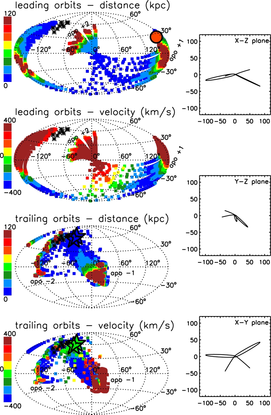
Figure 10 presents the results for the integrations of initial conditions within the Galactic escape speed run in the spherical version of the potential through two (future/past) apocenters leading/trailing the observed stars. The apocenters in the leading (upper pair of panels) and trailing (lower pair of panels) orbits stand out clearly in red when color coded by distance from the Galactic center (top in each pair of panels). As found in Section 3.4, although these distances can be substantially overestimated for the leading debris (and possibly underestimated for the trailing debris), we expect the angular locations of the apocenters—in particular the ones closest in orbital phase to the observed stars (indicated by +1 and −1)—to provide useful indications of the locations of associated apocentric clouds. Indeed the locations of the closest apocenters was similar (i.e., to within tens of degrees) for our test cases in both spherical and triaxial potentials. Moreover, any unbound orbits were predicted to leave the Galaxy in the same portion of the sky as these first apocenters. In contrast, the morphology and location of the apocenters further apart in orbital phase from the observed data (i.e., +2 and −2) were found to vary more substantially (in some case by up to 100°in angular separation) across our test cases. While this calls into question the utility of our current predictions for searching for debris at such large separations in orbital phase, it does emphasize the power that any future associations that can be made across more than a single oscillation in radial phase would have on constraining the potential (as also noted by Varghese et al. 2011).

Figure 10. Sample orbit (right panels) and Aitoff projections (left panels) for the leading (top pair of left panels) and trailing (bottom pair of left panels) orbits calculated from initial conditions generated from the PDF shown in Figure 9. The right panels follow the integrations for ±1.5 Gyr, and the left panels show debris for two leading/trailing apocenters. The Aitoff projections on the left are color coded for distance (upper of each pair of panels) and velocity (lower of each pair of panels). Black points indicate the positions of stars in Group D. Colored stars are detections of velocity groups, with the colors showing distance and velocity estimates from Newberg et al. (2007) and Vivas et al. (2008). The circle indicates the location and distance of group A11 from Sharma et al. (2010).
Download figure:
Standard image High-resolution imageIt is apparent from a comparison of the paths of leading and trailing orbits in Aitoff projections in Figure 10 with Figure 8 that none of the predicted apocenters exactly match the locations of well-known clouds. The predicted apocenters are at too great distances and low latitudes for most of the surveys. However, one of the possible groups found by Sharma et al. (2010; named "A11") is only slightly offset in angular position from the predicted location of the first apocenter along the leading orbits (around (l, b) = (164°, 25°)), and at a distance slightly less than that predicted (consistent with expectations for leading debris)—as indicated by the orange circle in the top panel of the figure. Moreover, our predicted apocentric location is actually slightly beyond the edge of Sharma et al.'s (2010) survey boundary (dictated by the Galactic Midplane Zone of Avoidance), plausibly explaining the perceived angular offset. We conclude that, while Sharma et al. (2010) felt that the proximity of A11 to both the disk and the edge of their chosen survey area called into question A11's authenticity as a real structure, our own tentative connection to local debris provides motivation for a follow-up spectroscopic survey. If such a survey revealed a strong velocity gradient across the structure going from positive to negative vGSR both the validity of the A11 group, and its possible connection to our own Group D could be confirmed.
Another plausible connection that can be made is to one of the velocity structures seen in the direction of the VOD and VSS—though not to those specific overdensities themselves. The colored stars in the lower pair of panels indicate the locations, distances, and line-of-sight speeds for one of these velocity peaks derived from spectroscopic surveys in the direction of the VSS (Newberg et al. 2007; Vivas et al. 2008; Brink et al. 2010) that best matches our predictions. The coincidence between our predictions and the distances and velocities of this observed feature is striking.
It is also interesting to note that, while we do not match the RV of the VSS in this region, the orbital properties derived using proper motion measurements for the VSS itself by Casetti-Dinescu et al. (2009) are remarkably similar (apocenter of ∼90 kpc, pericenter of ∼11 kpc, and an orbital inclination of 58°) to the one illustrated in the top panels of Figure 10. This agreement is somewhat circumstantial, because there is a wide range of orbital properties among the predicted orbits more generally. Nevertheless, if we could indeed connect the model and observations as representing two separate pericentric passages, we would have an even greater chance of knowing where to look for related clouds.
4.3. Group E
As for Group D, the stars used in our analyses for Group E were chosen to stand out from the disk in either motion or abundances or both, and to be part of the distinct sequence picked out by eye in the vGSR/cos b versus l plane. They are highlighted with black symbols in the lower panel of Figure 1, with circles indicating those particular stars that have additional high-resolution spectroscopy. A total of 13 stars in our medium-resolution spectroscopic survey fulfilled these combined constraints and five of those have high-resolution spectra. In addition, in a subsequent observing run at MDM observatory we found yet another star that fell along the Group E sequence, and we include it in our analysis and all figures.
4.3.1. Derivation of Full-space Motion
The left and middle panels of Figure 11 show the results of running the MCMC analysis (see Section 3.3) on the line-of-sight velocity data in the heliocentric rest frame. The PDF contours enclose a smaller area of velocity space than Group D that is also far from the local escape speed. The right panel shows the angular momentum of particles generated from these PDFs. As with Group D, there is no clear-cut association between any of the local, previously known moving or angular momentum groups and our derived properties for Group E.
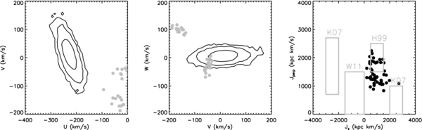
Figure 11. Same as Figure 9, but for Group E stars.
Download figure:
Standard image High-resolution image4.3.2. Predictions for and Possible Associations with Clouds
Figure 12 presents the results for the integrations of initial conditions generated from the MCMC PDF for the motion of Group E in the version of our potential with a spherical halo component. As for Group D, the predictions up to the first leading/trailing apocenters are very similar in the different potentials, but quite different at orbital phases farther away from the initial conditions of the integrations.
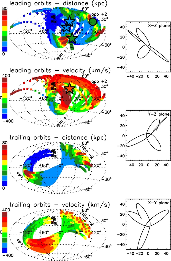
Figure 12. Same as Figure 10, but generated from PDF shown in Figure 11. Black points indicate the positions of star in Group E. Colored stars are detections of the HerAq cloud reported in Belokurov et al. (2007). The green line in the top-left panel indicates the overdense region, and distance of RR Lyraes found in SDSS "Stripe 82" (Watkins et al. 2009). The circle shows the location and distance of M giant group A13 reported in Sharma et al. (2010).
Download figure:
Standard image High-resolution imageThe most promising cloud association for Group E from our orbit predictions is where the leading orbits plunge across the disk plane to their first apocenters just below the disk around (l, b) ∼ (30°, −20°)—as apparent in the top-left panel of Figure 12. The crossing and apocenter overlap the region where the HerAq was first discovered using SDSS photometry (see Figure 1 of Belokurov et al. 2007, for a striking view). While SDSS does not cover the location of our predicted apocenter, Belokurov et al. (2007) demonstrated that low-latitude SEGUE observations at a longitude l = 50° clearly show the star counts to be denser and more distant below the disk (at (l, b) ∼ (50°, −15°)) than just above, in the same sense as our predictions. The colored stars indicate where Belokurov et al. (2007) detected and made distance estimates for this overdensity, and the colored, dashed line indicates the locations and distances of RR Lyraes in SDSS Stripe 82 (Watkins et al. 2009). The bulk of the population in both studies is found in the range 10–20 kpc, although Watkins et al. (2009) detected stars as far as 60 kpc. While these populations are somewhat closer than the apocenters of the orbit integrations, we expect the leading orbits to overestimate the distances. Moreover, our orbit integrations suggest that the densest, central region may sit outside the SDSS or SEGUE footprints, at lower Galactic latitude and longitude.
Belokurov et al. (2007) also looked at the region 20° < b < 55°, 20° < l < 75° and found a population of stars associated with this overdensity with a peak line-of-sight motion ∼180 km s−1 (see orange star in leading orbit's velocity panel). Once again, the observed region is offset from our stream predictions, but the motion is in the same sense expected.
The SDSS distance and velocity observations lie near our leading orbital paths, suggesting that the pericentric stream represented by Group E, as well as the SDSS photometric and spectroscopic detections, might both be skirting the edge of a much larger structure. If this is indeed the case, then we should be able to find the densest region of the cloud around the predicted apocenter in the M giant catalog. Note that both Belokurov et al. (2007) and Watkins et al. (2009) estimated average metallicities for their detections of [Fe/H] ∼ −1.5 (with a tail to values as high as [Fe/H] = −1), which is too low for a large fraction of M giants in the stellar population. In fact, HerAq was not found in the same regions as SDSS by the Sharma et al. (2010) group-finding analysis of the M giants from 2MASS, which could either be a consequence of the low metallicity of the population or because of the faint magnitude cut (Ks > 10) that was applied to the M giants to limit foreground contamination. Sharma et al. (2010) did find a group of M giants at low, negative Galactic latitude and longitude (labeled "A4" in their work), but the majority were clearly part of the Sgr trailing debris stream.
Figure 13 re-assesses the nature of overdensities in the M giants by plotting the number of stars in the latitude range 30 < |b| < 50 as a function of Galactic longitude for each of the Galactic hemispheres. These distributions are expected to be symmetric about the Galactic center in the absence of any substructure. The presence of Sgr debris is obvious in the ∼10° wide peaks at l ∼ −10° in the north (top panel) and l ∼ 10° in the south (bottom panel). Figure 8 shows the path of Sgr debris responsible for these peaks. In addition, at positive longitudes in the south there is an apparent extension of the Sgr overdensity to higher longitudes, as seen by the counts around l ∼ 20°.

Figure 13. M giant star counts in the latitude range 30° < |b| < 50° for the northern (upper panels) and southern (lower panels) Galactic hemispheres.
Download figure:
Standard image High-resolution imageFigure 14 assesses whether this extension is indeed part of the Sgr debris by plotting the distribution of Ks apparent magnitudes for two samples of M giants selected from those represented in the bottom right-hand panel of Figure 13: those in the range 0° < l < 15° (dotted histogram) and those in the range 15° < l < 40° (solid histogram). Comparison of these distributions clearly shows that the stars at higher longitudes (where we expect HerAq to be) are at systematically brighter magnitudes than those in the Sgr region, which suggests that the former stars could be dominated by a distinct debris structure. Moreover, Majewski et al. (2003) commented on a local peak in star counts at this position along the Sgr trailing debris (25° < Λ☉ < 50° in their Figure 13). In a subsequent spectroscopic survey, Majewski et al. (2004) found a dozen stars in this area, within 5 kpc of the Sgr orbital plane, but with velocities inconsistent with the Sgr tails and instead falling in the range −100 < vGSR < 100 (see their Figure 2(a))—just as might be expected for HerAq cloud debris turning around at apocenter.

Figure 14. Distribution in apparent Ks magnitudes for M giants in the bottom right-hand panel of Figure 13 in the longitude ranges 15° < l < 40° (solid) and 0° < l < 15° (dotted).
Download figure:
Standard image High-resolution image
Overall, we conclude that Group E may plausibly represent the pericentric stream associated with the HerAq cloud, and with a tentatively identified, diffuse cloud of M giants around (l, b) = (20°, −30°) in particular. A velocity map across the face of the cloud could confirm this association: Sgr debris in the region would have GSR velocities decreasing slowly as |b| increases along the tail; in contrast, our predictions for the Group E debris in this region are for a steep gradient from negative to positive velocities as l increases.
Finally, looking further along the leading orbits to the second apocenter in our predictions we find another connection, to structure "A13" discovered in the group-finding analysis of the more distant 2MASS M giant sample by Sharma et al. (2010). The structure (Figure 12, filled circle in upper left panel) coincides in both position and distance with our expectations for Group E debris. Nevertheless, we consider this connection more speculative than the one made to HerAq, both because our predictions are less consistent in different potentials at these wide separations in orbital phase, and because the reality of the A13 structure itself is considered uncertain. Discovery of a systematic velocity gradient across structure A13, with motions along the line of sight decreasing toward lower Galactic latitudes, would bolster both the physical reality of A13 and its association with Group E.
4.4. Alternative Interpretation of Group E
As noted above, the predictions for locations of other debris associated with both Groups D and E rely on the assumption that the sequences picked out by eye from Figure 1 result from a pericentric stream passing with a single velocity through the survey volume. In a concurrent independent study of nearby K giants, a sequence at a similar location in longitude/velocity space to Group E has been identified (Majewski et al. 2012). However, this sequence has been interpreted, using N-body simulations, as resulting from stars associated with the disruption of the globular cluster ωCen (which has also been postulated to be the surviving nucleus of a dwarf galaxy; see Bekki & Freeman 2003), turning around near the apocenters of their orbits. The proposed different scenarios for the K and M giant sequences can be distinguished using observations of proper motions (stars connecting to clouds would have much high proper motions) or by comparing the chemistry of these stars (Smith et al. 2000; Majewski et al. 2012, found ωCen stars to have abnormally high barium abundances at M giant metallicities).
5. SUMMARY AND CONCLUSIONS
This paper presents a first investigation into the possibility of connecting RV–longitude sequences of stars found in surveys of the nearby Galaxy to large-scale inhomogeneities in star counts from photometric surveys of the outer Galactic halo. If such connections can be made, they would bolster our confidence in the physical interpretation of the local star sequences as pericentric streams associated with apocentric clouds of tidal debris.
Our analysis of simulations of satellite accretion demonstrates that
- 1.sequences in velocity across the sky found in spectroscopic surveys may indeed be the signature of streams of debris passing through the local volume;
- 2.the full-space motions of the streams can be estimated directly from these sequences;
- 3.even with ∼15 stars in a sequence, integrations of the (very uncertain) derived full-space motions in any reasonable potential provide useful predictions for the locations and motions of other associated debris;
- 4.the predictions differ significantly with different shapes for the Galactic potential once integrations are separated by more than one radial orbit from the initial conditions.
Applying these ideas to two possible sequences (Groups D and E) found in a spectroscopic survey of M giants reveals plausible associations with various prior detections of cloud-like overdensities—in particular, for Group D to structure A11, and for Group E to HerAq and A13.
We conclude that follow-up spectroscopic surveys of these more distant cloud-like structures should allow us to confirm or rule out these tentative associations. If associations are confirmed, these debris systems would be the first comprehensive maps of satellite disruption around the Milky Way for progenitors following eccentric orbits and fill in a knowledge of Galactic accretion history that is currently missing. Moreover, the maps would have comparable extent to those of Sgr's debris streams, and hence provide additional strong constraints on the shape and depth of the Galactic potential. Finally, knowledge of the velocity of streams of stars passing at high speed through the solar vicinity would provide insight into the interpretation of direct dark matter detection experiments and help constrain the nature of dark matter itself.
The work of K.V.J. and A.A.S. on this project was funded in part by NSF grants AST-0806558 and AST-1107373. A.A.S. acknowledges the support of Columbia's Science Fellows. NSF grant AST-0807945 provided partial support for S.R.M. All the authors thank the other members of the "Cloud Hopping" team for their ongoing contributions to this program: Rachael Beaton, Jeff Carlin, Sébastien Lépine, Ricky Patterson, Ricardo Muñoz and Whitney Richardson.