


ABSTRACT
We investigate the launching of jets and outflows from magnetically diffusive accretion disks. Using the PLUTO code, we solve the time-dependent resistive magnetohydrodynamic equations taking into account the disk and jet evolution simultaneously. The main question we address is which kind of disks launch jets and which kind of disks do not? In particular, we study how the magnitude and distribution of the (turbulent) magnetic diffusivity affect mass loading and jet acceleration. We apply a turbulent magnetic diffusivity based on α-prescription, but also investigate examples where the scale height of diffusivity is larger than that of the disk gas pressure. We further investigate how the ejection efficiency is governed by the magnetic field strength. Our simulations last for up to 5000 dynamical timescales corresponding to 900 orbital periods of the inner disk. As a general result, we observe a continuous and robust outflow launched from the inner part of the disk, expanding into a collimated jet of superfast-magnetosonic speed. For long timescales, the disk's internal dynamics change, as due to outflow ejection and disk accretion the disk mass decreases. For magnetocentrifugally driven jets, we find that for (1) less diffusive disks, (2) a stronger magnetic field, (3) a low poloidal diffusivity, or (4) a lower numerical diffusivity (resolution), the mass loading of the outflow is increased—resulting in more powerful jets with high-mass flux. For weak magnetization, the (weak) outflow is driven by the magnetic pressure gradient. We consider in detail the advection and diffusion of magnetic flux within the disk and we find that the disk and outflow magnetization may substantially change in time. This may have severe impact on the launching and formation process—an initially highly magnetized disk may evolve into a disk of weak magnetization which cannot drive strong outflows. We further investigate the jet asymptotic velocity and the jet rotational velocity in respect of the different launching scenarios. We find a lower degree of jet collimation than previous studies, most probably due to our revised outflow boundary condition.
Export citation and abstract BibTeX RIS
1. INTRODUCTION
Jets as highly collimated beams of high-velocity material and outflows of comparatively lower degree of collimation and lower speed are an ubiquitous phenomenon among astrophysical objects. Jets are powerful signs of activity and are observed over a wide range of luminosity and spatial scale. Among the jet sources are young stellar objects (YSOs), micro-quasars, active galactic nuclei (AGNs), and most probably also gamma-ray bursts (Fanaroff & Riley 1974; Abell & Margon 1979; Mundt & Fried 1983; Rhoads 1997; Mirabel & Rodríguez 1994). The common models of launching, acceleration, and collimation work in the framework of magnetohydrodynamic (MHD) forces (see, e.g., Blandford & Payne 1982; Pudritz & Norman 1983; Uchida & Shibata 1985), although the details of the process are not fully understood.
Jets and outflows from YSO and AGNs affect their environment, and, thus, the formation process of the objects that are launching them. Numerous studies investigate effects of such feedback mechanisms in star formation and galaxy formation (see, e.g., Banerjee et al. 2007; Carroll et al. 2009; Gaibler et al. 2012). However, a quantitative investigation of how much mass, momentum, or energy from the infall is actually recycled into a high-speed outflow needs to resolve the innermost jet-launching region and to model the physical process of launching directly. This is the major aim of the present paper.
According to the current understanding, accretion and ejection are related to each other. One efficient way to remove angular momentum from a disk is to connect it to a magnetized outflow. This has been motivated by the observed correlation between signatures of accretion and ejection in jet sources (see, e.g., Cabrit et al. 1990; Hartigan et al. 1995).
The overall idea is that the energy and angular momentum are extracted from the disk by an efficient magnetic torque relying on a global, i.e., large-scale magnetic field threading the disk. If the inclination of the field lines is sufficiently small, magnetocentrifugal forces can accelerate the matter along the field line. Beyond the Alfvén point Lorentz forces also contribute to the acceleration. The collimation of the outflow is thought to be achieved by magnetic tension due to a toroidal component of the magnetic field. Still, we have to keep in mind the fact that the toroidal field pressure gradient is de-collimating, and an existing external gas overpressure may contribute to jet collimation.
Before going into further detail, we wish to make clear that with jet formation we denote the process of accelerating and collimating an already existing slow disk wind or stellar wind in to a jet beam. With jet launching we denote the process which conveys material from radial accretion into a vertical ejection, thereby lifting it from the disk plane into the corona, and thus establishing a disk wind.
A vast literature exists on MHD jet modeling. We may distinguish (1) between steady-state models and time-dependent numerical simulations, or (2) between simulations considering the jet formation only from a fixed-in-time disk surface and simulations considering also the launching process, thus taking into account disk and jet evolution together.
Steady-state modeling has mostly followed the self-similar Blandford & Payne approach (e.g., Sauty & Tsinganos 1994; Contopoulos & Lovelace 1994), but fully two-dimensional models were also proposed (Pelletier & Pudritz 1992; Li 1993), some of them taking into account the central stellar dipole (Fendt et al. 1995; Paatz & Camenzind 1996). Further, some numerical solutions have been proposed by Königl et al. (2010), Salmeron et al. (2011), and Wardle & Königl (1993) in weakly ionized protostellar accretion disks that are threaded by a large-scale magnetic field as wind-driving accretion disks. They have studied the effects of different regimes for ambipolar diffusion or Hall and Ohm diffusivity dominance in these disk. (Self-similar) Steady-state models have also been applied to the jet-launching domain (Ferreira & Pelletier 1995; Li 1995; Casse & Ferreira 2000), connecting the collimating outflow with the accretion disk structure. In addition to the steady-state approaches, the magnetocentrifugal jet formation mechanism has been subject of a number of time-dependent numerical studies. In particular, Ustyugova et al. (1995) and Ouyed & Pudritz (1997) have demonstrated for the first time the feasibility of the MHD self-collimation property of jets. We note, however, that it was already 1985 when the first jet formation simulations were published, in that case for a much shorter simulation timescale (Shibata & Uchida 1985). Among these works, some studies investigated artificial collimation (Ustyugova et al. 1999), a more consistent disk boundary condition (Krasnopolsky et al. 1999), the effect of magnetic diffusivity on collimation (Fendt & Čemeljić 2002), or the impact of the disk magnetization profile on collimation (Fendt 2006). In the aforementioned studies, the jet-launching accretion disk is taken into account as a boundary condition, prescribing a certain mass flux or magnetic flux profile in the outflow. This is a reasonable setup in order to investigate jet formation, i.e., the acceleration and collimation process of a jet. However, such simulations cannot reveal the efficiency of mass loading or angular momentum loss due to flux from disk to jet, or answer the question of which kind of disks do launch jets and under which circumstances.
It is therefore essential to extend the jet formation setup and include the launching process in the simulations. Numerical simulations of the MHD jet launching from accretion disks have been presented first by Kudoh et al. (1998) and Casse & Keppens (2002), treating the ejection of a collimated outflow out of an evolving-in time resistive accretion disk. Zanni et al. (2007) further developed this approach with emphasis on how resistivity affects the dynamical evolution. An additional central stellar wind was considered by Meliani et al. (2006). Further studies were concerned with the effects of the absolute field strength or the field geometry, in particular investigating field strengths around and below equipartition (Kuwabara et al. 2005; Tzeferacos et al. 2009; Murphy et al. 2010). The latter were long-term simulations for several hundreds of (inner) disk orbital periods, providing sufficient time evolution to also reach a (quasi) steady state for the fast jet flow.
Finally, we would like to emphasize the fact that jets and outflows are observed as bipolar streams. Jets and counter-jets appear typically asymmetric with only very few exceptions. One exception is the protostellar jet HH 212 showing an almost perfectly symmetrical bipolar structure (Zinnecker et al. 1998). So far, very few numerical simulations investigating the bipolar launching of disk jets have been performed. Among them are the works of von Rekowski et al. (2003) and von Rekowski & Brandenburg (2004) which even included a disk dynamo action. Recent publications consider asymmetric ejections of stellar wind components from an offset multi-pole stellar magnetosphere (Long et al. 2008, 2012; Lovelace et al. 2010). It is therefore interesting to investigate the evolution of both hemispheres of a global jet–disk system in order to see whether and how a global asymmetry in the large-scale outflow can be governed by the disk evolution. This has not been done so far.
In a series of two papers, we will address both the detailed physics of MHD jet launching (Paper I) and the bipolarity aspects of jets (Paper II). In the present paper (Paper I), we investigate the details of the launching, acceleration, and collimation of MHD jets from resistive magnetized accretion disks. We investigate how the mass and angular momentum fluxes depend on the internal disk physics applying long-lasting global MHD simulations of the disk–jet system. We hereby investigate different resistivity profiles of the disk. This paper is organized as follows. Section 2 is dedicated to MHD equations and to describing the numerical setup, the initial and boundary conditions of our simulations. The general evolution of jet launching and the physical processes involved are presented in Section 3 with the help of a reference simulation. Section 4 is then devoted to a parameter study comparing jets from different setups.
In Paper II, we will present the bipolar jet simulations, discussing their symmetry properties, and how symmetry can be broken by the intrinsic disk evolution.
2. MODEL SETUP
We model the launching of an MHD outflow from a slightly sub-Keplerian disk, initially in pressure equilibrium with a non-rotating disk corona.
As illustrated in Figure 1, matter is first accreted radially along a disk surrounding a central object and is then loaded on to the magnetic field lines. The large-scale magnetic field is threading the disk and thereby connects the accretion and ejection processes.
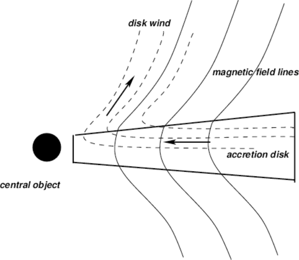
Figure 1. Schematic display of the outflow launching process from accretion disks. Matter (dashed lines) is accreted along the disk surrounding a central object and is loaded on to the magnetic field lines (solid lines). The emerging disk wind is further accelerated and collimated into a high-velocity beam (jet formation).
Download figure:
Standard image High-resolution imageOur main goals are
- 1.to determine the relevant mass fluxes (mass ejection and accretion rate) and to study the influence on them by the leading physical parameters, such as magnetic diffusivity and magnetic field strength,
- 2.to determine the resulting jet geometry—that is the asymptotic jet radius and opening angle, along with the size of the jet-launching area of the disk and the asymptotic jet velocity.
We will in a follow-up paper further extend our setup into two hemispheres, to investigate the launching of bipolar jets and their symmetry characteristics. The relevant mass and energy fluxes for accretion and ejection are of essential interest for feedback mechanisms in star or galaxy formation. With our highly resolved simulations of the innermost regions of these objects we intend to quantify these properties for a range of possible parameters.
2.1. MHD Equations
For our numerical simulations, we apply the MHD code PLUTO 3.01 (Mignone et al. 2007), solving the conservative, time-dependent, resistive, inviscous MHD equations, namely, for the conservation of mass, momentum, and energy,
Here, ρ is the mass density,  is the velocity, P is the thermal gas pressure,
  is the magnetic field, and Φ = −GM/R is the gravitational potential of the central object of mass M, with the spherical radius
  . In general, the magnetic diffusivity is defined as a tensor
  (see Section 2.5). The evolution of the magnetic field is described by the induction equation,
with the electric current density  given by Ampère's law
  . The cooling term Λ can be expressed in terms of Ohmic heating Λ = gΓ, with
  , and with g measuring the fraction of the magnetic energy that is radiated away instead of being dissipated locally. For simplicity, here we adopt g = 1. The gas pressure follows an equation of state P = (γ − 1)u with the polytropic index γ and the internal energy density u. The total energy density is
Our simulations are performed in axisymmetry applying cylindrical coordinates. The CENO3 algorithm as third-order interpolation scheme is used for spatial integration (Del Zanna & Bucciantini 2002) together with a third-order Runge–Kutta scheme for time evolution and an HLL Riemann solver. For the magnetic field evolution, we apply the constrained transport method (FCT) ensuring solenodality  .
.
2.2. Units and Normalization
Throughout the paper distances are expressed in units of the inner disk radius ri, while pd, i and ρd, i denote the disk pressure and density at this radius, respectively. The index "i" refers to a number value at the inner disk radius at z = 0 and time t = 0.
In Appendix A, we show for comparison the astrophysical scaling for YSO jets and AGN jets. Typically, ri < 0.1 AU for YSO and ri < 10 Schwarzschild radii for AGNs. Naturally, we cannot treat any relativistic effects of AGN jets with our non-relativistic setup. Velocities are measured in units of the Keplerian speed vK, i at the inner disk radius. Time is measured in units of ti = ri/vK, i, which can be related to the Keplerian orbital period τK, i = 2πti. Pressure is given in units of pd, i =  2ρd, iv2K, i. The magnetic field is measured in units of Bi = Bz, i. As usual we define the aspect ratio of the disk as the ratio of the isothermal sound speed to the Keplerian speed, both evaluated at disk mid-plane, ≡ cs/vK.5 For a more details see Appendix A.
2.3. Initial Setup—Disk and Corona
We define initial conditions following a setup applied by other authors previously—a magnetically diffusive accretion disk is prescribed in sub-Keplerian rotation, above which a hydrostatic corona in pressure balance with the disk is located (Zanni et al. 2007; Murphy et al. 2010). The coronal density is chosen several orders of magnitude below the disk density, thus implying an entropy and a density jump from disk to corona. However, contrary to previous authors (Zanni et al. 2007; Tzeferacos et al. 2009; Murphy et al. 2010), we do not apply an initial vertical velocity profile in the disk and only prescribe a radial velocity profile. We have seen that for our long-term simulations the whole disk system adjusts to a new dynamical equilibrium which does not depend on the vertical profile of the initial velocity distribution.
2.3.1. Initial Disk Structure
We prescribe an initially geometrically thin disk with = H/r = 0.1 which is itself in vertical equilibrium between thermal pressure and gravity.
We follow the standard setup employed in a number of previous papers (Zanni et al. 2007; Murphy et al. 2010).
As initial disk density distribution we prescribe
(Murphy et al. 2010), while the initial disk pressure distribution follows:
The disk is set into slightly sub-Keplerian rotation accounting for the radial gas pressure gradient and advection,
following Murphy et al. (2010), but neglecting viscosity.
In our setup the initial poloidal velocity is imposed by hand following the prescription of Zanni et al. (2007):
Simulations with initially vanishing disk accretion resulted in the same asymptotic inflow–outflow evolution. Starting with a disk inflow as in Equation (9), the inflow–outflow structure is established on a shorter timescale.
2.3.2. Structure of the Coronal Region
Above the disk, we define an initially hydrostatic density and pressure stratification (the so-called corona),
The parameter δ ≡ ρc/ρd quantifies the initial density contrast between disk and corona. We adopt δ = 10−4.
2.3.3. Magnetic Field Distribution
The initial magnetic field is prescribed by the magnetic flux function ψ following Zanni et al. (2007):
Here, Bz, 0 measures the vertical field strength at (r = ri, z = 0). The magnetic field components are calculated by rBz = ∂Ψ/∂r and rBr = ∂Ψ/∂z.
2.4. Numerical Grid
The computational domain spans a rectangular grid region applying a purely uniform spacing in the radial direction and a uniform-plus-stretched spacing vertically (Figure 2). We have run simulations in two different resolutions (see Table 1). For the low-resolution simulations, the domain extends to (96 × 288) inner disk radii ri on a grid of (1500 × 3200) cells, resulting in a resolution of Δr = 0.064. For the high-resolution simulations, the resolution is increased to 0.025 at the cost of being limited to a smaller domain of (50 × 180)ri. For all simulations presented here, a uniform grid is used for the magnetically diffusive disk.6

Figure 2. Computational domain consisting of two grids and a set of different boundary conditions. The computational domain covers (1500 × 1200) uniform grid cells on a physical domain of (r × z) = (96.0 × 80.0)ri. Another 2000 stretched grid cells are attached in the vertical direction 80.0 < z < 288.0. For the high-resolution simulations, a physical domain of (50.0 × 50.0)ri is covered with (2000 × 2000) grid cells to which another 2000 stretched grid cells are attached in the vertical direction between 50.0 < z < 180.0.
Download figure:
Standard image High-resolution imageFor the typical disk model applied with = 0.1 the low resolution provides only 2 grid cells per disk scale height at the inner disk radius, while for somewhat larger radii, say at r = 5, we have about 10 cells per disk scale height. In the high-resolution runs, the disk resolution is increased by a factor 2.5. As discussed by Murphy et al. (2010), the low resolution barely resolves the jet-launching disk surface layer of the very inner disk, where steep gradients in density, pressure, and diffusivity are present. Here, numerical diffusivity is supposed to play a role and we have devoted a section to investigating this effect.
In order to follow the jet outflow over long distances and in order to provide a sufficient mass reservoir for disk accretion a large domain would be desirable. In order to resolve the wind-launching area, a high resolution would be required. However, as mentioned before, PLUTO in its current version does not allow for diffusive MHD simulations in a stretched grid. Furthermore, we experience that for large domains together with stretched grids (implying an elongated shape of the outer grid cells) the code had difficulties solving the conservative equation and the simulations crashed.
2.5. Boundary Conditions
For the boundary conditions, axisymmetry on the rotation axis and equatorial symmetry for the disk mid-plane are imposed. At the upper z boundary, we use the standard PLUTO outflow boundary condition (zero gradient), but at the outer radial boundary condition, we apply a modified outflow condition as derived by Porth et al. (2011) in order to avoid artificial collimation. Most essential is the internal boundary enclosing the origin which we call a sink.
2.5.1. Internal Boundary—A Central Sink
We prescribe a sink for the mass flux in the very inner region of the domain. The sink is essential for the following reasons. First, the numerically problematic singularity at the origin can be hidden by this internal boundary. Second, the central sink allows the accretion flow to be absorbed through the disk and thus, emulate a central accreting object.
The sink is numerically introduced as an internal boundary condition, located on the region r < ri and z < zs.7 The internal boundary conditions defined at the right and top sides of the sink have significant impact on the simulation. If ill-defined, spurious effects arise during the early evolution. For the right side of the sink, we impose accretion conditions implying a zero gradient for pressure, density, and the vertical velocity component. For vϕ and Bϕ, a first-order extrapolation (constant gradient) is imposed which ensures an angular momentum decrease across the boundary which is essential for accretion. To allow for accretion further and also to minimize feedback from the sink to the domain, we constrain min in the ghost cells for the radial velocity component. We assume that the magnetic flux is not advected into the central object, and we impose Eϕ = 0. The normal component of the magnetic field is calculated from the solenodality condition along both sides of the sink.
On the top of the sink, we prescribe the initial local value for the gas pressure. In order to avoid evacuation of the regions close to the symmetry axis, we impose a density of 110% to the initial local density. Effectively, this condition replenishes the mass into the domain near to the axis to overcome numerically difficult low densities.
2.5.2. Outer Boundary Conditions
An essential point of our setup is to impose a proper outflow boundary at the outer boundary of the domain in r-direction avoiding artificial collimation forces. Here, we have implemented a current-free outflow condition (see Appendix B) which avoids spurious collimation by Lorentz forces and which has been thoroughly tested in our previous papers (Porth & Fendt 2010; Porth et al. 2011; Vaidya et al. 2011). In order to enable a long-term disk–jet simulation requiring a long-living disk accretion, we need to provide a sufficiently long-lasting mass reservoir. This could be realized by (1) a prescribed mass inflow, (2) a local mass replenishment, or (3) providing a large mass reservoir for jet-launching part of the accretion disk by extending the outer disk radius to large radii. All these approaches have been chosen in the literature. We decided to follow option (3) and provide a sufficiently high-mass reservoir outside of the inner launching region by extending the computational grid (and thus the outer disk radius) up to about 100 inner disk radii. Similar approaches haven been applied by Murphy et al. (2010) and Long et al. (2012).
We will see below (Section 3.2) that our approach is working well, but has, however, its limits if applied for long-lasting simulations. During about 5000 dynamical time steps, we lose about 30%–40% of the disk mass due to ejection and accretion and due to unwanted mass loss across the outer disk boundary.
2.6. The Disk Magnetic Diffusivity
A dissipative effect is required for steady-state accretion in order to allow matter to diffuse across the magnetic field threading the disk. Magnetic diffusivity allows the mass flux to cross the field lines and thus allows for accretion along the disk. We consider the magnetic diffusivity to be turbulent in nature, or "anomalous," and, thus, cannot be calculated self-consistently in our setup. The origin of the turbulent magnetic diffusivity is usually referred to being caused by the magnetorotational instability (MRI; Balbus & Hawley 1991, 1998) in a moderately magnetized disk.8
Nevertheless, we argue that as we load turbulently diffusive disk plasma into the outflow, it is natural to assume that the outflowing material is initially turbulent as well. Therefore, we have the option of applying a diffusive scale height Hη = ηr larger than the thermal scale height H = r of the disk, supposing that the turbulent disk material lifted into the outflow will remain turbulent for a few more scale lengths until turbulence decays. It is clear that the strong magnetization in the upper layers of the disk will prevent generation of turbulence by, e.g., the MRI, and will also quench the turbulence in the outflowing material. Without going into detail we may estimate the timescale for the decay of the turbulence potentially existing in the outflowing material as follows. The decay of (helical) MHD turbulence follows a power law EM ∼ t−n, where EM is the magnetic energy and the power-law index depends on further details but is in the range of n = 1/2–2/3 (Brandenburg & Nordlund 2011). Simulations indicate that MHD turbulence decays as fast as the hydrodynamic turbulence on a few eddy turnover times (Cho et al. 2002). With τη ⩾ H/cS = r/cS = r1/2 (in code units), we find a timescale for the decay of MHD turbulence launched from the disk into the outflow of, e.g., τη(r = 5) ⩾ 3, thus in the range of half an orbital period. This must be compared to the kinematic timescale for the jet launching. If we consider the propagation of the initially slow disk wind over a few disk pressure scale heights τwind(r = 5) ≃ H/vwind ≃ 0.5/0.05 = 10, we find that this time is of the order of a few eddy turnovers. Also, we will later see that jet launching is a rapid process with an outflow having been established after a few dynamical time steps.
Given the essential role of the magnetic diffusivity for wind/jet launching, we decided to investigate the launching process for different strengths and different scale heights of diffusivity. We have run simulations for a variety of combinations of parameter values, but for the sake of comparison, in this paper, we show results for diffusive scale height values, η = 0.1, 0.2, 0.3, and 0.4.
Formally, we apply an α prescription (Shakura & Sunyaev 1973), similar to previous works (see, e.g., Zanni et al. 2007). We assume the diffusivity tensor to be diagonal with the non-zero components

Here, we have defined a poloidal magnetic diffusivity ηp ≡ ηϕϕ = ηp, if(r, z) and the toroidal magnetic diffusivity ηϕ ≡ ηrr = ηzz = ηϕ, if(r, z), respectively,9 with a function f(r,z) describing the diffusivity profile.
As is known from the literature, an anisotropic magnetic diffusivity is required to obtain stationary solutions (Wardle & Königl 1993; Ferreira & Pelletier 1995; Ferreira 1997). Most of the numerical simulations followed that approach and did find a stationary state from their simulations as well (see, e.g., Zanni et al. 2007; Tzeferacos et al. 2009; Murphy et al. 2010). Note that simulations of Casse & Keppens (2002, 2004) apply an isotropic diffusivity and also reach a steady state.
We define an anisotropy parameter by the ratio of the toroidal to poloidal diffusivity components, χ = ηϕ, i/ηp, i. For the diffusivity function f several options can be considered. For the simulations in this paper, we apply
where ηp, i and ηϕ, i govern the strength of magnetic diffusivity. The Alfvén speed  and the disk thermal scale height H(r) = cs(r, z = 0)/ΩK(r, z = 0) are both calculated along the mid-plane. The parameter η measures the scale height of the disk magnetic diffusivity, similar to the hydrodynamic disk scale height parameter η = Hη/r. For the present paper, we decided not to evolve the diffusivity profile in time. We find that since both the disk scale height H and the Alfvén speed vA vary as the disk evolves, the strength of diffusivity may vary substantially from the initially prescribed value (up to a factor 10). This highly nonlinear feedback may disturb the progress of our simulation such that an artificially high diffusivity may be derived which will affect the numerical time stepping. A constant-in-time prescription of diffusivity simplifies our aim of disentangling the governing physical processes involved in jet launching.
In Paper II, presenting truly bipolar jet launching, we will discuss further models for the magnetic diffusivity.
We stress again the importance of providing the reader with the actual number values of the magnetic diffusivity applied.10 If we consider a ηϕ, i ∼ 1 together with a maximum Alfvén speed in the disk of about 10−2 (located at the inner disk radius), this gives a maximum disk diffusivity of about η(r, z)i ≃ 0.01–0.1, through all the simulations. Figure 3 shows the distribution of the magnetic diffusivity. The diffusivity is mainly concentrated in the disk, increases with disk radius (consistent with a decreasing temperature or ionization degree with radius), and decreases with height resembling the transition from a cool disk to an ideal MHD outflow.
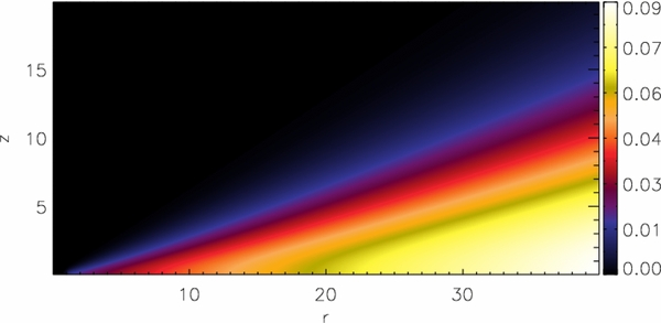
Figure 3. Distribution of the turbulent magnetic diffusivity ηp = ηp, if(r, z) in the disk–jet system for the reference simulation (see Equation (13)). Here, the diffusive scale height is Hη = 0.4r.
Download figure:
Standard image High-resolution image2.7. Main Simulation Parameters
The simulations are governed by a set of non-dimensional parameters for the following physical quantities.
- 1.The magnetic field strength defined by plasma-β, and its initial geometry defined by the "bending" parameter m.
- 2.The magnetic diffusivity, with the three parameters ηϕ, i, ηp, i, andη governing its strength, anisotropy, and the diffusivity scale height.
- 3.The initial density contrast between disk and corona δ.
- 4.The initial disk thermal scale height parameter = H/r.
An overview of these parameters is shown in Table 1 (first half) for the simulations presented in this paper. The second part of Table 1 shows the main dynamical quantities resulting from our simulations and will be discussed below. Table 2 shows similar numbers for the simulations of different diffusive scale heights.
Table 1. Input Parameters and Derived Dynamical Parameters of our Simulation Runs Following a Magnetic Diffusivity Profile Equation (13) with a Scale Height of the Disk Diffusivity η = 0.4
| Case 1 | Case 2 | Case 3 | Case 4 | Case 5 | Case 6 | Case 7 | Case 8 | Case 9 | Case 10 | |
| Δr | 0.064 | 0.064 | 0.064 | 0.064 | 0.064 | 0.025 | 0.025 | 0.064 | 0.064 | 0.064 |
| Δz | 0.066 | 0.066 | 0.066 | 0.066 | 0.066 | 0.025 | 0.025 | 0.066 | 0.066 | 0.066 |
| η |
0.4 | 0.4 | 0.4 | 0.4 | 0.4 | 0.4 | 0.4 | 0.4 | 0.4 | 0.4 |
| ηp, i | 0.03 | 0.01 | 0.15 | 0.09 | 0.03 | 0.03 | 0.03 | 0.03 | 0.03 | 0.03 |
| ηϕ, i | 0.09 | 0.03 | 0.09 | 0.27 | 0.01 | 0.09 | 0.09 | 0.09 | 0.09 | 0.09 |
| χ | 3 | 3 | 3/5 | 3 | 1/3 | 3 | 3 | 3 | 3 | 3 |
| β | 10 | 10 | 10 | 10 | 10 | 5000 | 10 | 50.0 | 250 | 500 |
| rjet, z = 180 | 43.8 | 73.8 | 24.46 | 28.57 | 33.19 | ... | ... | 47.8 | 50.0 | 34.13 |
| rjet, z = 60 | 25.01 | 38.41 | 15.37 | 17.72 | 25.02 | 21.69 | 19.6 | 27.54 | 24.18 | 17.22 |
| rl | 3.8 | 8.2 | 3.0 | 4.2 | 3.0 | ... | 3.5 | 2.8 | 0.8 | 0.7 |
| vjet, z = 170 | 0.4 | 0.23 | 0.85 | 0.56 | 0.8 | 0.47 | 0.42 | 0.56 | 0.49 | 0.27 |
| vjet, z = 280 | 0.45 | 0.3 | 0.92 | 0.61 | 0.9 | ... | ... | 0.5 | 0.89 | 0.22 |
| ζjet, 1a | 2.37 | 0.013 | 5.28 | 5.1 | 2.58 | 0.89 | 4.6 | 1.56 | 0.32 | 2.08 |
 |
0.0005 | 6 × 10⁻⁶ | 0.0002 | 0.0002 | 0.0007 | 5 × 10⁻⁵ | 0.0008 | 0.0001 | 0.0004 | 0.0002 |
| ζjet, 2 | 2.90 | 0.3 | 4.45 | 6.7 | 2.28 | ... | ... | 2.46 | 0.42 | 1.84 |
 |
0.001 | 0.0002 | 0.0003 | 0.0004 | 0.001 | ... | ... | 0.0003 | 0.0006 | 0.0004 |
 b b |
0.015 | 0.022 | 0.0038 | 0.0035 | 0.022 | 0.001 | 0.013 | 0.005 | ... | ... |
 |
0.008 | 0.016 | 0.001 | 0.001 | 0.007 | 0.005 | 0.009 | 0.004 | ... | ... |
 |
0.5 | 0.7 | 0.2 | 0.2 | 0.31 | ... | 0.6 | ... | ... | ... |
| ξ | 0.3 | 0.5 | 0.09 | 0.09 | 0.1 | ... | 0.39 | ... | ... | ... |
 |
0.008 | 0.005 | 0.002 | 0.002 | 0.027 | 0.005 | 0.005 | 0.008 | ... | ... |
 |
0.03 | 0.01 | 0.0025 | 0.005 | 0.034 | 0.0 | 0.016 | 0.008 | 0.0 | 0.0 |
 |
0.038 | 0.015 | 0.004 | 0.007 | 0.06 | 0.005 | 0.021 | 0.017 | ... | ... |
| Lkin | 1 × 10⁻⁴ | 9 × 10⁻⁶ | 1.3 × 10⁻⁴ | 7.4 × 10⁻⁵ | 4 × 10⁻⁴ | 5.5 × 10⁻⁶ | 7.1 × 10⁻⁵ | 3.7 × 10⁻⁵ | 1.9 × 10⁻⁴ | 10−6 |
Notes. Displayed are the input parameters of grid resolution Δr, Δz, magnetic poloidal and toroidal diffusivity ηp, i and ηϕ, i, the diffusivity anisotropy χ, and the plasma-beta parameter β. The following outflow parameters are derived from our numerical simulations: the asymptotic jet radius rjet, calculated as mass flux weighted (see Equation (17)), the launching radius rl, the typical speed of the outflow, vjet, the average collimation degree ζjet (see Equation (18)), the mass accretion rate  and mass ejection rate
  , the ejection index ξ, the diffusive scale height η, the kinetic and magnetic angular momentum losses by the outflow,
  and
and  , respectively, as well as the total angular momentum loss
  , and its asymptotic kinetic luminosity
  . All parameters are given in code units.
aThe collimation degree is measured from two different areas, ζjet, 1 enclosing 0 ⩽ r ⩽ 40, 0 ⩽ z ⩽ 160, and ζjet, 2 with the area 0 ⩽ r ⩽ 80 and 0 ⩽ z ⩽ 250.
bThe mass flux values for the two simulation cases 9 and 10 with high βi are omitted due to their highly perturbed behavior.
. All parameters are given in code units.
aThe collimation degree is measured from two different areas, ζjet, 1 enclosing 0 ⩽ r ⩽ 40, 0 ⩽ z ⩽ 160, and ζjet, 2 with the area 0 ⩽ r ⩽ 80 and 0 ⩽ z ⩽ 250.
bThe mass flux values for the two simulation cases 9 and 10 with high βi are omitted due to their highly perturbed behavior.
Download table as: ASCIITypeset image
Table 2. Comparison Between Different Diffusive Scale Heights
| Case 1 | Case 11 | Case 12 | Case 13 | |
| η |
0.4 | 0.1 | 0.2 | 0.3 |
| Δr | 0.064 | 0.064 | 0.064 | 0.064 |
| Δz | 0.066 | 0.066 | 0.066 | 0.066 |
| ηp, i | 0.03 | 0.03 | 0.03 | 0.03 |
| ηϕ, i | 0.09 | 0.09 | 0.09 | 0.09 |
| χ | 3 | 3 | 3 | 3 |
| β | 10 | 10 | 10 | 10 |
| rjet, z = 180 | 43.8 | 73.3 | 56.4 | 48.4 |
| rjet, z = 60 | 25.01 | 45.8 | 39.2 | 34.4 |
| rl | 3.8 | 7.2 | 7.2 | 6.2 |
| vjet, z = 170 | 0.46 | 0.35 | 0.33 | 0.41 |
| vjet, z = 280 | 0.53 | 0.46 | 0.41 | 0.47 |
 |
0.015 | 0.024 | 0.022 | 0.018 |
 |
0.005 | 0.015 | 0.015 | 0.01 |
 |
0.01 | 0.005 | 0.009 | 0.01 |
 |
0.033 | 0.015 ± 0.01 | 0.02 ± 0.003 | 0.028 |
Notes. Shown are some of the physical properties mentioned in Table 1 for different diffusive scale height runs which have been carried out up to t = 2000.
Download table as: ASCIITypeset image
3. MHD JET LAUNCHING
Before presenting detailed results of our parameter study of jet-launching conditions, we will first discuss the general physical processes involved considering our long-term reference simulation (case 1). This simulation will then be compared to simulations applying (1) different diffusivity profiles, (2) a higher grid resolution, and (3) different magnetic field strength (see Table 1). A similar setup will then be used to launch bidirectional outflows, without the constraint on hemispheric symmetry (see Paper II).
3.1. General Evolution
Our reference simulation case 1 is carried out up to t = 5000 dynamical time, corresponding to 796 inner disk orbital periods. It is thus one of the longest simulations considering MHD jet launching. This huge time period corresponds, however, only to three rotations at a radius r = 40 ri and to (only) one rotation at the outermost part of the disk r = 96 ri. Consequently, while the inner part of the disk, and thus the outflow evolving from that part, has reached a steady-state situation, the outer disk corona is still dynamically evolving. We will therefore focus our discussion mainly on the inner disk areas.
The time evolution of density together with the magnetic field is shown in Figure 4. Note that we do not show field lines integrated from certain footpoint radii, but magnetic flux contours. This allows us to visualize the diffusion and advection of the magnetic field as a consequence of the disk evolution.

Figure 4. Time evolution if the jet–disk structure for reference simulation case 1. Shown is the evolution of the mass density (color) and the poloidal magnetic field (contours of poloidal magnetic flux Ψ for the levels 0.01, 0.03, 0.06, 0.1, 0.15, 0.2, 0.26, 0.35, 0.45, 0.55, 0.65, 0.75, 0.85, 0.95, 1.1, 1.3, 1.5, and 1.7) for the dynamical times t = 0, 500, 1000, 2000, and 3000. The dark lines indicate the slow-magnetosonic (dashed), the Alfvén (solid), and the fast-magnetosonic (dot-dashed) surfaces at t = 3000. The electric current lines are shown for t = 500 (green solid lines).
Download figure:
Standard image High-resolution imageThe magnetic diffusivity distribution determines the coupling between the plasma and magnetic field, and, thus, affects the mass loading into the outflow. Since the high diffusivity is in the outer part of the disk, the coupling is weaker, and, thus, the mass loading less efficient. As a general result we observe a continuous and robust outflow launched from the inner part of the disk, expanding into a collimated jet.
Figure 5 shows the poloidal velocity distribution in jet and disk, and the normalized poloidal velocity vectors indicating the direction of the mass fluxes.
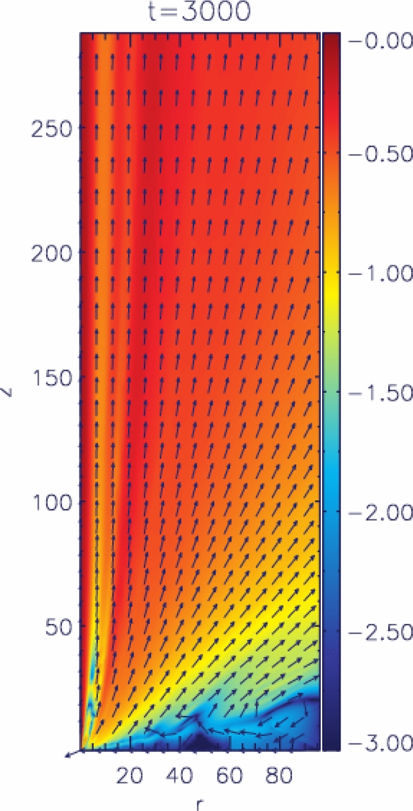
Figure 5. Accretion–ejection poloidal velocity map at t = 3000 for reference run case 1. Shown is vp distribution in logarithmic scale overlaid with arrows of the normalized poloidal velocity vectors indicating the direction of the flow,  .
.
Download figure:
Standard image High-resolution imageThe outflow is accelerated to superfast-magnetosonic speed (see the magnetosonic surfaces indicated in Figure 4)
A bow shock develops at the interface between the outflow and the surrounding hydrostatic corona. As the outflow propagates, the initial corona is swept out of the computational domain together with the bow shock. While the interaction with the ambient gas plays a role within the first evolutionary steps, the long-term evolution of the outflow—its acceleration and collimation—is purely determined by the force balance within the outflow and the physical conditions of the launching region.
3.2. Disk Structure and Disk Mass Evolution
As jets are launched from disks, the disk evolution is itself an essential part of the jet evolution and must be carefully considered. It is expected that the jet mass flux would somewhat correspond to the disk accretion rate (which would also depend on the actual mass of the disk).
Our simulations show that the disk evolution is complex, with smooth accretion phases followed by more turbulent stages. The time evolution of the accretion stream ρvr is shown in Figure 6. We see that accretion starts first at small radii and fully establishes after t = 1000. Accretion shocks and vortices may destroy the quasi-steady-state situation. Close to the outer disk radius, mass is lost through the outer boundary. At late evolutionary stages we see a complex pattern in the ρvr distribution indicating small shock and turbulent motion within the disk.

Figure 6. Time evolution of the accretion disk. Shown is the radial mass flux (ρvr) in the disk for reference run (case 1) for the dynamical times t = 0, 1000, 3000, and 5000.
Download figure:
Standard image High-resolution imageNevertheless, the negative mass fluxes in Figure 6, together with the negative velocity vectors in Figure 5 clearly indicate that accretion is established throughout the whole disk.
We now discuss the time evolution of the disk mass for our reference simulation. In order to measure the disk mass, we need to carefully define the control volume defining a corresponding "disk surface." Here, we consider as disk surface the location where the mass density at each radius falls bellow 10% of the mid-plane density (because of the vortex motion we could not use the negative velocity as a proxy for accretion). Measuring the mass contained in subsequent disk rings dM/dr = 2πrρdz, we see that most of the mass is indeed stored within the outer disk areas (Figure 7, top). We can identify two essential factors affecting the long-term disk evolution. First, the mass reservoir in the outer disk has decreased, mainly due to outwards mass loss across the outer disk boundary. Second, the mass of the inner jet-launching disk has also decreased, due to both outflow activity and accretion into the sink.

Figure 7. Time evolution of the disk mass. Shown is the radial profile of the mass distribution dM/dr (integrated mass per disk ring, in code units) at times t = 0, 3000, and 5000 (top), and the time evolution of the total disk mass Md normalized to the initial disk mass Md, i for integration radii r2 = 50 and 96 (bottom).
Download figure:
Standard image High-resolution imageComparing the mass content of the disk at the initial and final stage, we find that the total disk mass decreases from M ≃ 520 at t = 0 to M ≃ 320 at t = 5000 (in code units). Integrating the mass loss by accretion and ejection into the jet (see Figure 7) over 5000 dynamical time steps, we find a total mass loss of M ≃ 75. The difference, i.e., M ≃ 125, is the mass which is lost from the outermost disk in vertical and radial directions.
In other words, a substantial amount of the disk mass is lost from the very outer part of the disk and does not directly influence the jet formation. The disk mass which is lost from the inner part is partly lost as disk wind/jet, partly accreted into the sink and partly replenished by accretion from outer radii.
The time evolution of the disk mass gives a similar picture (Figure 7, bottom). Integrated over the whole domain, the disk loses about 38% of its mass until t = 5000 in the reference simulation case 1. If we decrease the integration domain (outer radius r = 50), the inner disk loses less mass while part of its mass is being accreted from outer disk radii. In general this implies that up to time t = 5000, there is still sufficient mass to support the accretion process, but also that the disk mass shows a considerable decrease which may have changed the internal disk properties. Thus, for an even longer-lasting simulation one would have to invent another mass source for the disk accretion (e.g., by a physical mass inflow boundary condition at the outer disk radius properly taking into account angular momentum transfer, or a floor density distribution in the disk).
Along with the hydrodynamic disk evolution, the magnetic field distribution evolves, subject to the competing processes of advection and diffusion. This also changes the launching conditions, as the overall profiles of plasma-β, resp. magnetization, are affected. Figure 8 displays the time evolution of the magnetic flux surface Ψ = 0.1 for reference simulation case 1, initially rooted at the radius r = 2.0. We see that this flux surface is first moving (diffusing) outward "driven" by magnetic pressure gradient and tension, and then, once disk accretion has established again moves inward being advected with the mass flux. After about t = 3000 both processes balance and a quasi-steady-state situation in the system evolution is reached. Considering simply flux conservation, we may estimate the change in poloidal magnetic field strength and the corresponding change in magnetic diffusivity and plasma-β.
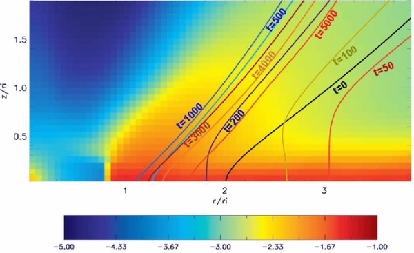
Figure 8. Diffusion and advection of magnetic flux. Shown is the evolution of the magnetic flux surface ψ = 0.1 for times t = 0, 50, 100, 200, 500, 1000, 3000, 4000, and 5000 (colored lines) for reference simulation case 1. This flux surface is initially rooted at (2, 0). Superimposed is the density distribution at t = 5000.
Download figure:
Standard image High-resolution imageEstimating an average field strength  and a corresponding magnetic flux
  , flux conservation tells us that Ψt = 1000 ≈ ψt = 50. Therefore,
  , since this flux surface (e.g., Ψ = 0.1) is now rooted at a different radius. With the increased poloidal magnetic field strength the Alfvén speed vA ∼ Bp increases, and, thus, also the magnetic diffusivity parameterized as η ∼ vA. Thus, we expect that in previous work (e.g., Zanni et al. 2007; Tzeferacos et al. 2009) the actual (time-dependent) value of the magnetic diffusivity may differ substantially from its initial value. We believe that this will impact the derived mass fluxes. A similar estimate can be made for the plasma-β or magnetization. Since β ∼ B−2, the increase in plasma-β is by a factor 100, which is also expected to affect the jet formation severely. We will come back to this point later when we compare different parameter runs.
3.3. Accretion Rate and Ejection Efficiency
The main goal of this paper is to investigate what fraction of the mass accretion is loaded into the outflow, and how the mass loading is affected by various disk parameters. The derived mass ejection-to-accretion ratio can be an important ingredient for studies of AGN or YSO feedback, or another similar self-regulating outflow scenario.
Efficient accretion is feasible only if angular momentum is sufficiently removed. Since we do not consider physical viscosity in our simulations, angular momentum removal from the disk is mostly accomplished by the torque of the magnetized disk wind. Therefore, in our simulations disk accretion can only work if a disk wind has been established. In the following we discuss the inflow and outflow rates in our disk–jet simulations, concentrating first on the reference run (case 1).
In order to calculate the integrated properties of inflow and outflow, such as mass flux or angular momentum flux, we need to carefully select the integration domain.11 The derived fluxes depend strongly on the choice of the integration boundaries—thus, on how we distinguish between material belonging to accretion or ejection. In reality, there is no disk surface, but a smooth transition between accretion and ejection. The initial setup of a thin disk with aspect ratio = 0.1 dynamically evolves in time, and so does the disk surface.
Our control volume to measure the disk accretion and ejection rates is defined by an axisymmetric sector enclosed by two surfaces perpendicular to the equatorial plane located at r = r1 and r = r2, and two other surfaces being the disk mid-plane, and a surface s1 which is close by and parallel to the initial disk surface (see Figure 9). We usually adopt r1 = 1.0.
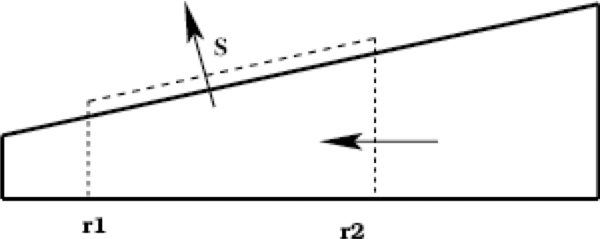
Figure 9. Control volume to measure the accretion and ejection rates in the jet–disk structure. Integration is at/between the radii r1 and r2 along the disk. The integration surface denoted by S is inclined and is parallel to the initial disk surface.
Download figure:
Standard image High-resolution imageThe accretion rate is then calculated as
where the parameter a controls the scale height of the integration and H = H(r, t = 0) = r is the initial thermal scale height of the disk. Considering the evolution of the large-scale disk velocity (see Figure 6), we have chosen a = 1.6 for our reference simulation. Similarly, we calculate the ejected mass flux as

where the integration is performed along the inclined surface area S from r1 to r2 considering the area element  .
.
The time evolution of the accretion and ejection rate for the reference simulation is shown in Figure 10. We have calculated the accretion and ejection rates for different sizes of the integration domain (thus with different outer radius r2). We observe that for small radii, the accretion rate saturates at an approximately constant value. For the outer parts of the disk, however, a longer dynamical time is required for the disk to evolve into a new dynamical steady state. This is visible in the time evolution of the accretion rates—for increasing radii r2 = 3, 5, and 10, the time when the plateau phase is reached, is increasing to t = 300, 800, and 1500. Beyond the plateau phase, the mass fluxes slightly decrease, most probably due to the overall decrease of the disk mass itself, and the subsequent change in the internal disk dynamics. The accretion rates at large radii are larger than those at smaller radii—the mass difference is ejected as outflow. For the control volume with larger r2 the ejection rate increases, which is simply a consequence of the increased integration area.
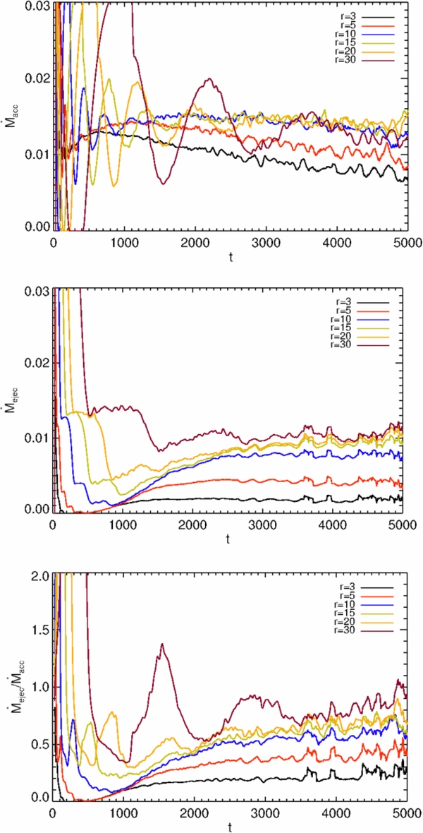
Figure 10. Time evolution of the mass fluxes. Shown is evolution of accretion rate (top), the ejection rate (middle), and the ejection-to-accretion ratio (bottom) for the reference simulation case 1, all in code units. Colors indicate mass fluxes calculated for increasing outer radii of the control volume, r2 = 3, 5, 10, 15, 20, and 30.
Download figure:
Standard image High-resolution imageThe last panel in Figure 10 shows the ejection-to-accretion rate  . Again, depending on the size of the control volume this fraction changes. Although the outflow quickly evolves from the disk surface, and extends soon to large radii, several orbital periods are required to establish full accretion. At earlier times and for large radii, the accretion process is not fully established, resulting in somewhat arbitrarily high ejection-to-accretion ratios even above unity. For the inner part of the disk within radii <10, about 60% of the accreting material is diverted into the outflow for our reference simulation. This is a large fraction and similar to simulations in the literature, but definitely more than derived in steady-state models (Pelletier & Pudritz 1992; Ferreira & Pelletier 1995). For the other cases we have investigated, also smaller rates were obtained (see below).
Applying a radially self-similar approximation of the MHD equations, Ferreira & Pelletier (1995) have introduced a so-called ejection index ξ,
essentially resulting from local mass conservation (where ri = r1 and re = r2 in our notation). With self-similar solutions, Ferreira (1997) constrained the ejection index to 0.04 < ξ < 0.08. In comparison, for our reference run we find both larger numerical values and also a wider range for the ejection index, 0.1 < ξ < 0.5. Table 1 provides an overview of the ejection indexes we measured. We can apply our reference run to different astrophysical sources (see Appendix A), thus for a stellar jet with the central mass ≈1 M☉ and ρi ≈ 10−10, the accretion rate is ≈10−6 M☉ yr−1. This value for AGNs with the central mass ≈108M☉ and ρi ≈ 10−12 is about ≈7 M☉ yr−1.
3.4. Launching Forces and Outflow Formation
In order to investigate the launching, the acceleration and the collimation processes of the outflow, we now consider the forces acting in the disk-outflow system.
To identify the forces for acceleration and collimation explicitly, it is preferable to project them along or perpendicular to a certain flux surface, respectively. By comparing these projected force components, we may disentangle the dominant driving and collimation mechanism. Figure 11 shows the force components along a flux surface (field line) rooted at (5, 0), and also the critical MHD surfaces—the slow-magnetosonic, the Alfvén, and the fast-magnetosonic surface. The forces involved in driving the outflow are the centrifugal force FC, the Lorentz force FL, the gas pressure gradient FP, and gravity FG. Among them, the pressure gradient and the centrifugal force are de-collimating while gravity and Lorentz force have collimating components. The pressure gradient, centrifugal force, and Lorentz force also contribute to accelerate the outflow. In agreement with the literature, we see that upstream of the slow-magnetosonic point, the acceleration is mainly by the gas pressure gradient. For the superslow outflow, the Lorentz force and the centrifugal force dominate. For the superfast flow, the Lorentz force plays a major role. In the case of the collimating forces the situation is different. Before the Alfvén point, the de-collimating centrifugal force dominates. Beyond the Alfvén point the Lorentz force has a comparable contribution, and finally after the fast-magnetosonic point, the Lorentz force dominates and collimates the outflow. The Lorentz force behavior is a sign of the electric current distribution in the disk/jet system. It compresses the disk while collimating the corona.

Figure 11. Accelerating and collimating forces. Shown are the profiles of the parallel (top) and perpendicular (bottom) specific forces in logarithmic scale for simulation case 1 at time t = 1000 along the distance λ of the field line rooted at (5,0). Here FC, FG, FL, and FP denote the centrifugal force, gravity, the Lorentz, and the gas pressure gradient forces (all in absolute value), respectively. The vertical lines present the slow-magnetosonic (dashed line), the Alfvén (solid), and the fast-magnetosonic (dot-dashed) point, respectively.
Download figure:
Standard image High-resolution imageThe forces involved in launching the outflow are mainly the vertical gas pressure gradient, which counteracts the tension forces of the poloidal field, and gravity (see Figure 11). The thermal pressure gradient is always positive, and thus supports launching. It increases from the disk mid-plane to the surface and then decreases in the corona. The tension term is mostly negative, thus compressing the disk, and does not support launching. The magnetic pressure (toroidal component and total) are both positive above the disk, and, thus, may support the launching process. The toroidal component of the Lorentz force Fϕ, L provides the magnetic torque braking the disk, and loading the outflow with both angular momentum and energy (not shown). In order to brake the disk, the torque must be negative in the disk and change sign at the disk surface (Ferreira 1997). This is confirmed by our simulation.
Figure 12 shows for comparison the three main force components (top) and the net force (bottom). We see that in the disk the vertical force components almost balance, while above the disk a considerable net force remains which launches and accelerates the outflow. In the disk, the (positive) gas pressure is almost balanced by the (negative) Lorentz force. However, the gas pressure slightly prevails and counteracts gravity. Essentially the figure shows that launching is a process which happens at the disk surface. The outflow material is not lifted from the mid-plane into the disk wind. It is the disk material accreting along the disk surface that is loaded into the outflow. The net (specific) force which is responsible for launching and initial acceleration is about 10% of the value of the single force components.
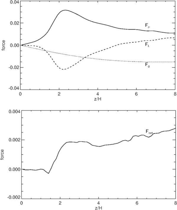
Figure 12. Launching forces of the outflow. Shown is the vertical profile of the vertical components of gravity, the pressure gradient force, and the Lorentz force (top), as well as the vertical profile of the net force (bottom) at time t = 1000 at a radius r = 5 for in case 1.
Download figure:
Standard image High-resolution image3.5. Jet Radius and Opening Angle
The radius of the asymptotic jet and its opening angle can be measured by the observations rather easily. Therefore, it is interesting to provide a comparison from the simulations. Simple energy conservation arguments tell us that jets with the observed kinetic energy must originate from a disk area very close to the central object. This is a fact which seems to hold for all astrophysical jet sources. We will later consider the question of how these asymptotic properties are related to the conditions of the jet-launching process. Here, we first provide a clear numerical definition of these properties and apply them to our reference simulation. In order to make a quantitative comparison, we need to define a "radius of the outflow." We suggest a definition of an axial mass-flux-weighted jet radius, measured at a certain distance z = zm from the source (see also Porth & Fendt 2010),
This radius measures the bulk of the mass flux contained in the jet at a specific distance zm from the mid-plane. In order to derive the jet-launching area, we now adopt that flux surface which follows the bulk of the mass flux, thus passing through the point (rjet(zm), zm), and trace the same flux surface back to the disk surface where it is rooted. This footpoint radius defines the launching area of the outflow. For reference run case 1, we find a mass-flux-weighted asymptotic jet radius for the high-velocity component of rjet ≃ 44 at zm = 180, corresponding to ≃ 4 AU for a protostellar scaling applying ri = 0.1 AU. For the jet-launching radius, we measure rl ∼ 0.4 AU in our reference run. Similarly, the launching area for the extended low-velocity component of the DG Tauri wind was measured by Anderson et al. (2003) as extending from ∼0.3 to 4 AU from the star. They invented a method relying on the MHD energy and angular momentum conservation along the jet. By comparing the observed kinetic energy and jet rotation they inferred the necessary disk rotation and launching area in the wind-launching region.
The asymptotic jet opening angle is the other jet characteristic. One way to measure the jet opening angle is by the inclination angle of the flux surface defined by the asymptotic jet radius as discussed above. Another measure of the collimation was suggested by Fendt (2006) who assigned an average collimation degree ζ of the outflow by comparing the vertical and radial mass fluxes in the outflow (applying a proper normalization per surface area of a cylinder of height z = zm and radius r = rm),

where only positive poloidal velocities are considered. Outflow collimation would simply imply that ζjet > 1. For our reference run, we find ζjet = 2.37 implying that about twice as much mass is propagating along the jet axis than away from the jet axis. For comparison, the flux surface which encloses the bulk of the jet mass flux has an (half) opening angle of about 10° at (r, z) = (44, 180), but collimates slightly more further downstream. We note that this definition is related also to the concentration of mass flux across the jet, and, thus, provides somewhat different information than the opening angle of the field lines. For example, a cylindrical jet with zero degree opening angle may have a narrow or a broad radial density or mass flux profile. With our definition the narrow mass flux would be interpreted as more collimated.
4. COMPARISON OF PARAMETER RUNS
In this section we compare simulations governed by different input parameters which rely on a magnetic diffusivity profile following Equation (13) with a scale height of the disk diffusivity Hη = ηr, grid resolution Δr, Δz, maximum magnetic poloidal and toroidal diffusivity ηp, i and ηϕ, i, the diffusivity anisotropy χ, and the plasma-beta parameter β (see Table 1). We understand these parameters as the governing parameters of jet launching from accretion disks. All simulations have been carried out up to t = 3000 (reference run up to t = 5000). We found that this time is sufficient to reach a quasi-steady state of accretion–ejection (roughly after t = 1000).
We first show a comparison of the global mass density distribution at t = 3000 for simulation setups resulting from a different strength η or different anisotropy χ of diffusivity, a different plasma-β, or a different grid resolution (Figure 13). The immediate result is that both the disk structure and the dynamical evolution of the outflow, change substantially compared to the reference run (case 1). Jet-like outflows have been formed in all cases, although in some cases like case 6 with β = 5000, or case 9 with β = 250, the outflow appears highly filamentary. Denser outflows are observed as in case 7 with higher resolution, or case 2 with lower diffusivity, or case 5 with lower toroidal diffusivity, while in other cases the outflow is more tenuous. Outflow and disk evolution are interrelated—a denser outflow thus implies a geometrically thinner accretion disk, as more of the accreting matter has been diverted into the outflow. The smoothness of the outflow varies for the different setups. We obtain a much more filamentary and perturbed structure for outflows for which the (physical or numerical) diffusivity in the disk is lower. A similar statement can be made for a low magnetic field strength.
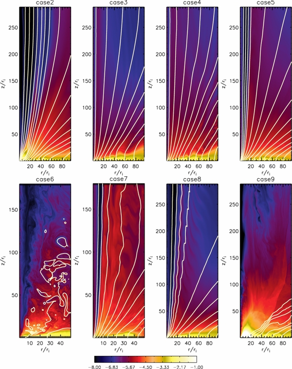
Figure 13. Comparison of different parameters runs (see Table 1) at t = 3000. Shown is the density distribution and the poloidal magnetic field (contours of magnetic flux for levels Ψ = 0.01, 0.03, 0.06, 0.1, 0.15, 0.2, 0.26, 0.35, 0.45, 0.55, 0.65, 0.75, 0.85, 0.95, 1.1, 1.3, 1.5, and 1.7) for simulation runs with rather low diffusivity (case 2), rather high poloidal diffusivity with anisotropy χ = 3/5 (case 3), rather high diffusivity strength (case 4), rather low toroidal diffusivity with anisotropy χ = 1/3 (case 5), simulations with a rather weak magnetic field with plasma-β = 5000 (case 6), plasma-β = 100 (case 8), plasma-β = 250 (case 9), and also a simulation with three times higher resolution (case 7), all to be compared to our reference simulation case 1, see Figure 4.
Download figure:
Standard image High-resolution imageWe now consider the main properties of the accretion–ejection system in a quasi-steady state for all simulation runs. The two most prominent physical quantities are the mass and the angular momentum fluxes. Similar to the mass fluxes defined in Equations (14) and (15) we integrate the ejection torque that is the torque exerted on the disk by the outflow applying the same control volume (see Section 3.3),
with the kinetic and magnetic angular momentum flux,  and
and  , carried by the outflow. Figure 14 shows the time evolution of the accretion rate (top) and the ejection rate (bottom) for the different cases. The accretion rate is calculated for radius r = 10 for all cases.12 For comparison, we show the corresponding vertical angular momentum flux evolution (Figure 15). For all cases investigated, accretion sets in after several hundreds of rotations and is fully established within t ≃ 1000. After some initial fluctuations, the accretion rate levels off into a steady state, depending on the physical parameters prescribed in the simulation.
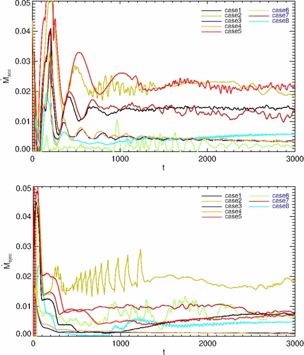
Figure 14. Comparison of mass fluxes for the different cases. Shown is the time evolution of the accretion–ejection rate (top) and the ejection rate (bottom) for simulation runs applying a different parameter setup (see Table 1).
Download figure:
Standard image High-resolution image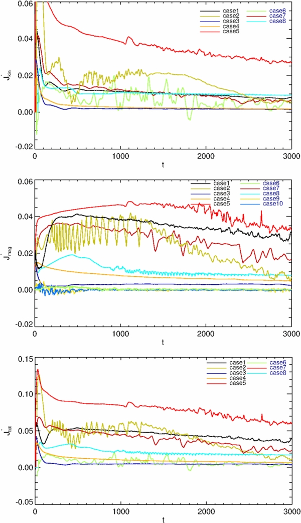
Figure 15. Comparison of angular momentum fluxes for the different cases. Shown is the time evolution of the vertical angular momentum flux from the disk, calculated for a control volume with r1 = 1.0 and r2 = 10.0 (see Table 1).
Download figure:
Standard image High-resolution imageDepending on the efficiency of the angular momentum transfer from the disk, the disk establishes a different accretion rate. We find that the simulation runs with the highest accretion rates, also have the highest angular momentum flux from the disk (Figures 14 and 15). These are the case 2 runs with rather low diffusivity and case 5 with rather low poloidal diffusivity, strongly indicating that with a low diffusivity and, thus, a strong coupling between field and matter, the MHD torque of the jet on the disk is most efficient, and subsequently leads to a more efficient disk accretion. Similarly, the high plasma-β (thus with a low field strength, simulations runs (cases 6, 8, 9, and 10)) exhibit a weak magnetic angular momentum removal and, consequently, are inefficient accretors (see Table 1). In summary, we find that the extraction of angular momentum from the disk by the outflow and accretion are clearly interrelated.
In the following sections, we discuss how the governing system parameters, such as diffusivity, plasma-β, and numerical resolution, affect the mass flux evolution.
4.1. Possible Impact of Numerical Diffusivity
Before we further investigate the physical effects, we discuss the results of our resolution study. Numerical diffusivity will add to the physical diffusivity, as it is a natural consequence of the finite-difference scheme applied in the PLUTO code. This effect could be particularly important in the jet-launching regime close to the disk surface where strong gradients in density, pressure, or magnetic diffusivity exist, and which may not be resolved. Murphy et al. (2010) have claimed that jet launching could be in fact present just due to numerical diffusivity.
In order to estimate the impact of numerical diffusivity we have repeated our reference simulation case 1 with a three times higher resolution (case 7), but with the same physical diffusivity and anisotropy parameter as for the reference simulation. We find that the leading disk and outflow properties are similar to the reference case. The accretion rate is slightly decreased from  (case 1) to
  (case 7), while the ejection rate is slightly increased from
  to
to  (see Table 1). Due to the smaller computational domain for the high-resolution simulation, we cannot compare the asymptotic jet radii (at z = 180); however, we can compare the radius of the bulk mass flux similar to Equation (17) for lower altitudes (at z = 60). The simulation with higher resolution seems to result in a slightly more collimated jet, with a jet radius of rjet = 19.6 compared to rjet = 25 for the reference simulation. This results in a similarly smaller jet-launching radius. The maximum jet velocities are just the same vjet = 0.5.
Figure 14 shows the time evolution of the mass fluxes. We see that the accretion rates and ejection rates for case 1 and case 7 saturate at the same level. It appears that the high-resolution simulation needs more time to establish an outflow, while the accretion evolves similarly in both runs. One may see indication for a slightly larger accretion rate for the low-resolution run, which would fit into the picture that the disk material can more easily diffuse across the field lines due to the numerical diffusivity.
The same picture holds for the angular momentum fluxes (see Figure 15), which are very similar for the kinematic part and slightly offset for the magnetic part.
4.2. Impact of the Magnetic Field Strength
There is a common agreement in the literature that jet formation requires a certain amount of magnetic flux to be present in the jet-launching regime. On the other hand, the maximum magnetic flux which can be supported by the accretion disk is limited by the disk equipartition field strength (we will neglect the question of the origin of the magnetic field in this paper).
We have also studied the impact of the magnetic field strength on jet launching, governed by the plasma-β parameter. We note that we start all simulations with the same magnetic field profile; however, due to diffusion and advection in the disk, the field distribution may change substantially.
The magnetic field strength determines the amount of magnetic energy which is available for jet acceleration and is directly interrelated with the length of the lever arm of the magnetic torque on the disk (e.g., Pelletier & Pudritz 1992).
Due to the larger magnetic torque in case of a strong field, the disk angular momentum could be removed more efficiently. In order to investigate these effects quantitatively, we will compare simulations with different plasma-β, such as case 1 with initial β = 10, case 8 with β = 50, case 9 with β = 250, and the weak field case 6 with β = 5000. Note that the plasma-β is, however, a space- and time-dependent function of the simulation, β = β(r, z, t) and not only a single parameter we prescribe initially at the inner disk radius. In the high plasma-β regime, the flow of matter controls the dynamical structure of the system. For all cases of a weak magnetic field, the disk–jet system evolution seems highly perturbed—visible in the global structure of the outflow (Figure 13, cases 6, 8, and 9).
Note that the regimes with high plasma-β are known to be dominated by the internal, turbulent torque, which is not taken into account in our simulations by an α-viscosity.
In particular, for cases 9 and 10, the mass flux evolution is exceptionally perturbed (so we decided not to include them in all plots and just show the magnetic angular momentum flux). Figure 15 proves that with increasing plasma-β, less angular momentum is removed from the disk, and, subsequently, the accretion rate is reduced. This is particularly visible when we compare the simulation with β = 50 with the reference run with β = 10. In the case of the weakest magnetic field, thus for the simulations with β = 250 and β = 5000, the magnetic angular momentum removal is close to negligible. For the weak field cases, the accretion rate decreases, and in cases 9, 10, and 6 no efficient accretion is observed. In summary, we confirm the hypothesis that efficient magnetocentrifugal jet driving requires a strong magnetic flux (i.e., a low plasma-β), together with a large enough magnetic torque in order to produce a powerful jet.
Simulation case 6 applies a very weak magnetic field with β = 5000. Figure 16 compares the two simulations: case 6 with the standard setup case 7 in high resolution. No smoothly structured outflow is obtained for case 6, but a highly turbulent outflow with non-negligible outflow speed and mass flux. Due to the weak poloidal field, the outflow in case 6 is super-Alfvénic right from the launching point, thus magnetocentrifugal acceleration cannot play a role. Interestingly, the size of the turbulent features increases with distance from the origin. Also the poloidal magnetic field is highly tangled (Figure 13). The mass flux we measure for case 6 is about  with outflow velocities of vjet ≃ 0.4. While the velocities are comparable to case 7 (or case 1 with lower resolution), the ejected mass flux is substantially lower (factor two). Accretion in case 6 is weak (the smallest of all simulations), consistent with the low angular momentum losses (the smallest of all simulations). The accretion rate is even smaller than the ejection rate (factor five), and we may call such a disk an ejection disk instead of an accretion disk.
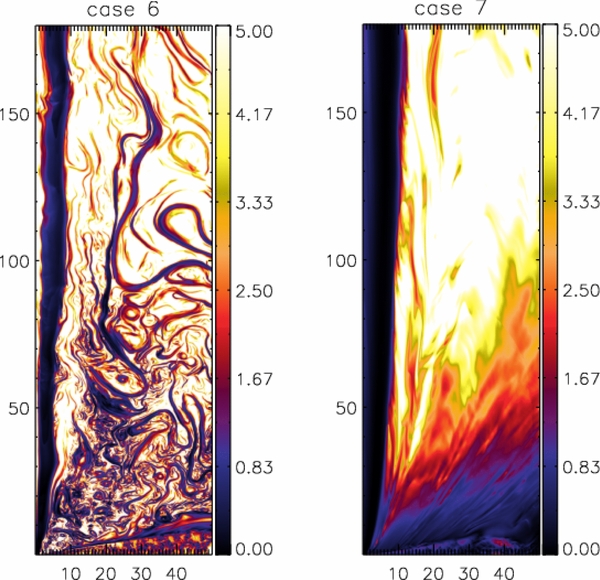
Figure 16. Comparison of outflow launching for low and high plasma-β cases. Display of the Alfvénic Mach number for two simulations with three times higher resolution. The left panel shows the weak field case β = 5000 (case 6). The right panel shows the strong field case β = 10 (case 7).
Download figure:
Standard image High-resolution imageThe question is: what is launching and accelerating such a turbulent, high plasma-β outflow? Our interpretation is that the initial acceleration to superescape speed is by the toroidal magnetic pressure gradient (induced by the differential rotation between the rotating disk and the static corona). When the bow shock has left the domain, this acceleration process decays, and the remaining outflow acceleration is due to weak Lorentz force (as we are in the super-Alfvénic regime). The vertical mass flux for case 6 (very weak field) is one order of magnitude below the mass flux in case 7 (with strong field β = 10), measured at the same altitude (see Table 1). In summary, launching conditions as in case 6 with β = 5000 do not produce a strong jet flow, but a light disk wind of superescape speed.
We point out that the physical regime of acceleration does not only depend on the field strength, but also on the mass flux. Magnetocentrifugal effects are more evident for outflows with low-mass flux, while in heavy jets the magnetic pressure gradient may play a substantial role (see, e.g., Anderson et al. 2005).
The relative field strength (measured by the plasma-β) is a function of space and evolves in time. The initial field and gas pressure distribution, denoted by the βi, is changed by the dynamical evolution including advection and diffusion of the disk magnetic field. Figure 17 shows the evolution of the plasma-β for case 1. It is clearly visible that the plasma-β along the disk surface changes substantially. The inner disk (for r < 15) reaches a steady state with a β somewhat higher than the initial value. Later, around t = 3000 when the disk mass decreases, the gas pressure decreases as well, resulting in a lower plasma-β in the disk corona. The disk corona therefore remains sufficiently magnetized and can support a fast jet. In case 1 the magnetic field structure reaches a steady state balanced by field diffusion advection.
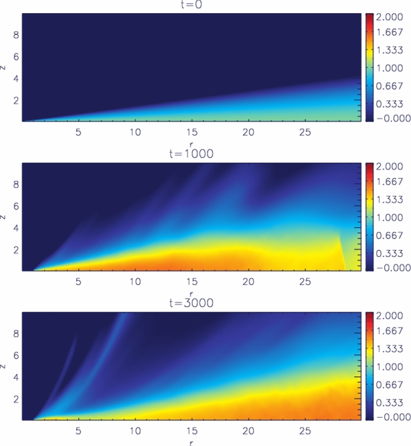
Figure 17. Time evolution of the plasma-β in the inner disk–jet system. Snapshots of the plasma-β distribution (in logarithmic scale) for case 1 at t = 0, 1000, and 3000.
Download figure:
Standard image High-resolution imageIn simulation case 7 with the same parameter setup but a higher resolution, a steady state is reached as well. However, even for late time steps the magnetic flux continues to diffuse outward. This is somewhat surprising since the numerical diffusion is smaller and cannot be the reason (Figure 18, top). For case 8 with the higher initial plasma-β, advection seems to dominate outward diffusion of flux. The poloidal field distribution reaches a steady state with a magnetic flux concentration close to the inner edge of the disk (Figure 18, bottom). Thus, this setup seems favorable for jet launching as well, although the initial plasma-β was high.
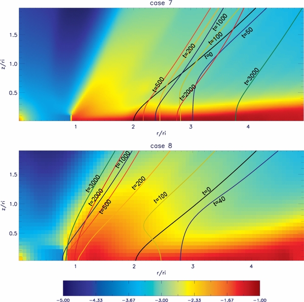
Figure 18. Advection and diffusion of magnetic flux over time. Shown is the evolution of the magnetic flux surface Ψ = 0.1 rooted initially at (r, z) = (2, 0), for case 7 (high resolution) and case 8 (β = 50). Colors show the density distribution at t = 3000 (logarithmic scale).
Download figure:
Standard image High-resolution imageAs an extreme example, for simulation case 9 with the initial β = 250 the plasma-β is considerably changed during the disk evolution. Case 9 shows very weak accretion (see the discussion above), so outward diffusion of magnetic flux dominates advection. Outward diffusion of flux implies a decrease of magnetic field strength. As a result the disk magnetization decreases and the plasma-β reaches number values above 105. Therefore, this disk is not able to launch strong jets. So far no steady state is achieved.
The interrelation between the magnetic field strength and outflow launching has been discussed by other authors (Tzeferacos et al. 2009; Murphy et al. 2010), indicating that regions with weak field are not able to generate an outflow, and that both the collimation degree and the ejection rate increase with stronger field. Murphy et al. (2010) have concluded that jet launching for cases of weak magnetization may be artificially supported by numerical diffusivity within the disk surface layer, which should heat the gas, producing additional gas pressure. They suggest that ejection is possible as the magnetization reaches unity at the disk surface due to the steep density decrease. No ejection is reported when the mid-plane magnetization becomes too small. Nevertheless, the asymptotic jet velocity remained too low to explain the observed jet's speed. From our simulations, we find that even for weak magnetization in the disk the disk corona is sufficiently magnetized for jet launching and, depending on the efficiency of mass loading, fast jets could be driven (for comparison, see Figure 17 for case 1). The mass loading depends on resistivity, and we will discuss this aspect in the next section.
We finally consider the possibility to observe the MRI in our simulations. This is interesting since we are dealing with magnetic fields of various strength in combination with a differentially rotating system. To generate the MRI in numerical simulations, two conditions are essential—a large enough (but not too large) plasma-β in the disk as to initiate instability, and also a grid of high enough resolution in order to avoid damping of small wavelengths. The wavelength of the most unstable MRI mode is given by λMRI = 2πvA, z/ΩK for a Keplerian rotation ΩK (see, e.g., Romanova et al. 2011). When we calculate this wavelength for a simulation with β = 10, we obtain λMRI ≃ 0.057, implying that we cannot resolve the MRI with our setup as the grid size is about half of the MRI wavelength.
We point out that the magnetic diffusivity applied in our simulations also contributes to suppressing the generation of MRI turbulence.
4.3. Magnetic Diffusivity Strength and Anisotropy
The strength and anisotropy of the magnetic diffusivity—controlled by the coefficients ηϕ, i, ηp, i, and χ (see Table 1)—are essential parameters governing the coupling between the magnetic field and the plasma. Efficient magnetocentrifugal driving requires strong coupling between the magnetic field and the rotating disk material, thus a rather low diffusivity. A similar argument holds for the launching by magnetic pressure gradient. On the other hand, mass loading from accretion to ejection requires a certain degree of diffusivity in order to transport mass across the field lines.
So far, no general model for the magnetic diffusivity distribution in disk–jet structures is available. In many simulations considering magnetocentrifugal-driven outflows, the outflow is governed by ideal MHD, while the diffusivity is confined to the disk. In order to investigate the impact of diffusivity on jet launching, we have therefore performed simulations with varying strength of the diffusivity components ηϕ, i and ηp, i.
We first compare simulations with the same anisotropy parameter χ = 3 as reference run case 1. In general, the strength of magnetic diffusivity governs the disk accretion rate. Our reference run case 1 reaches a quasi-steady state, establishing a balance between inward advection and outward diffusion of magnetic flux. This happens after t = 1000 and is disturbed again in the late stages of the dynamical evolution, most probably as a result of the change in the overall disk dynamics due to the decreasing disk mass. A change in diffusivity will also affect this balance. We now compare case 4 with higher and case 2 with lower diffusivity. In the less diffusive case, advection dominates and we obtain a higher accretion rate. We find that not only the accretion rate, but also the ejection rates are higher for disks with lower diffusivity. This trend is shown in Figure 19, where we display the accretion rate and also the ejection rate as a function of the poloidal diffusivity.

Figure 19. Mass flux  vs. poloidal diffusivity. Shown is the ejected jet mass flux (triangles) and the accretion rate (circles) as function of the poloidal diffusivity for simulations with the same magnetic field strength, i.e., case 1 (ηp, i = 0.03), case 2 (ηp, i = 0.01), case 3 (ηp, i = 0.15), case 4 (ηp, i = 0.09), and case 5 (ηp, i = 0.03).
Download figure:
Standard image High-resolution imageTwo physical processes affect the disk dynamics—advection and diffusion. In a less diffusive disk, the plasma is stronger coupled to the field and advection of magnetic flux dominates. Consequently, the magnetic flux surfaces are located further in the inner part of the disk, "rotate" faster, and a stronger Bϕ is induced. The stronger toroidal field may lead to a stronger acceleration of the outflow, by stronger Lorentz forces (either magnetic tension of pressure forces). In addition, by comparing the vertical profiles of net launching forces at t = 1000 for a less diffusive disk (case 2), and reference run (case 1), we find a larger net force in case 2 by which implies that more disk material can be lifted into the outflow.
This is exactly what we observe in the mass fluxes—the ejected mass flux in case 2 is two times the ejected mass flux in case 1. Note that a stronger Bϕ will impose stronger pinching forces ∼(Bϕ · ∇)Bϕ on the disk and the ejected material, thus opposing the loading process (as the toroidal tension has a component along the field line decelerating the outflow meterial). However, the magnetic pressure gradient of the toroidal field ∼∇B2ϕ has an outward directed component along the field line, thus supporting ejection. By comparing the vertical profiles of both terms for the two cases with β = 10 and β = 50, we find that (1) the toroidal magnetic field pressure gradient component along the field line is always dominating the pinching force of the toroidal field along the field line, and that (2) for higher plasma-β the (∇B2ϕ)z is larger than for the lower plasma-β case. Thus, in our simulations the toroidal field is supporting ejection.
In summary, although a certain magnitude of diffusivity is required for mass loading, the lower diffusivity allows for enhanced mass loading of accreting material into the outflow. Consequently, less diffusive disks tend to have higher ejection rates. This result is in agreement with the previous literature (Zanni et al. 2007).
Our simulations confirm that the strength of magnetic diffusivity does affect the asymptotic speed of the outflow. Figure 20 shows the typical jet velocity versus the poloidal diffusivity. Comparing different simulation runs (see Table 1), we find that the outflow from the less diffusive disk (case 2) remains slower, while the outflows formed from more diffusive disks (cases 3 and 4) are accelerated to higher speed. For case 2 with three times lower magnetic diffusivity, the asymptotic speed is reduced by ≈30%, while for case 4 with three times higher magnetic diffusivity the increase is about ≈30% (see Table 1). This is reasonable from a physical point of view, since in a weakly diffusive disk more material is diverted into the outflow. Thus, with the same amount of magnetic flux available, correspondingly less magnetic energy could be transferred per outflow mass unit. The more massive outflows are only accelerated to lower speed if launched with similar magnetization. Alternatively, a higher magnetic diffusivity, resulting in a weaker mass load, leads to a faster outflow.

Figure 20. Jet velocity vs. poloidal diffusivity at t = 3000. Shown is the typical jet velocity as a function of (but different) diffusivity, i.e., case 1 (ηp, i = 0.03), case 2 (ηp, i = 0.01), case 3 (ηp, i = 0.15), case 4 (ηp, i = 0.09), and case 5 (ηp, i = 0.03).
Download figure:
Standard image High-resolution imageWhen comparing our results with the previous literature, one should keep in mind that we have applied a mass flux weighted velocity which we consider as the typical velocity of the bulk mass flux. The velocity value is generally lower than the maximum speed we measure in the outflow and which is mostly given in the literature. While the typical speed ranges from about 0.5 to 0.9 (in code units), the maximum speed in the outflow ranges from 1.2 to 1.8 inner disk Keplerian velocities and is comparable to other results in the literature. Furthermore, we have detected a slight time evolution in the velocity (see also the mass flux evolution shown in Figure 14). In our reference run case 1, the maximum asymptotic speed varies from vp, max = 1.8 at t = 500 to vp, max = 1.2 for t > 1000. For comparison, Zanni et al. (2007) and Tzeferacos et al. (2009) give a maximum speed of vp, max ≃ 1.5–4.5 at t = 400.
Next, we investigate a possible impact of anisotropy in the diffusivity tensor, parameterized by χ. We compare case 1 and case 5 with the same polodial diffusivity ηp = 0.03, but with case 5 having a lower diffusivity in the toroidal direction. By comparing their leading properties (see Table 1), we find them to have quite similar properties. In particular, for both cases (with the same poloidal diffusivity) the ejection rates are also similar. However, case 5 with less toroidal diffusivity has a higher accretion rate.
Anisotropy of magnetic diffusivity also impacts the rotation of the outflow. It is believed that jets are rotating and the rotation is basically driven by the underlying disk rotation and the coupling between matter and field (Bacciotti et al. 2002; Anderson et al. 2003; Coffey et al. 2004; Fendt 2011). For a high toroidal diffusivity, the coupling is weak, and thus the acceleration in toroidal direction is also weak. With our simulations we can confirm this concept. Figure 21 shows the rotational velocity for the lower part of the jet. The outflow resulting from simulation case 1 with a nine times higher toroidal diffusivity shows a 50% lower rotation rate than for case 5. Similarly, the outflows in simulation case 4 with a three times higher toroidal diffusivity shows a 50% lower rotation rate than case 3.13
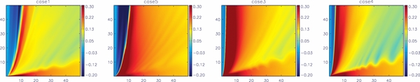
Figure 21. Outflow rotation and toroidal magnetic diffusivity. Shown is the rotational velocity vϕ of the inner disk–jet system at t = 3000 for simulation runs with different toroidal magnetic diffusivity, respectively, different anisotropy parameters χ, i.e., cases 1, 5, 3, and 4 (from left to right).
Download figure:
Standard image High-resolution imageWe observe a close correlation between the accretion rate  and angular momentum flux
  from the disk. In a system with higher angular momentum removal, a higher accretion rate is observed (Figure 15), with the accretion rate in case 5 being larger than for case 1, and for case 1 larger than for case 3. This confirms the common belief that in order to obtain higher accretion rates, a more efficient angular momentum removal is required.
To discuss the interrelation between collimation and diffusivity, we again apply a collimation degree by comparing the directed mass fluxes (see Equation (18)). As a general result we find that outflows launched from disks of higher poloidal diffusivity ηp are more collimated. This interrelation is displayed in Figure 22.
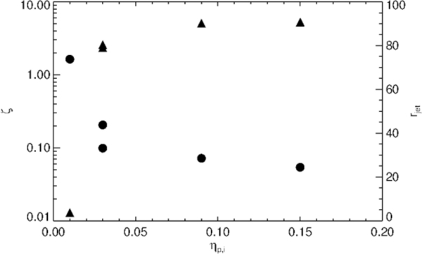
Figure 22. Collimation degree and jet radius vs. poloidal diffusivity. Shown is the collimation degree ζ (filled triangles) and the mass-flux-weighted jet radius rjet (filled circles) over the poloidal diffusivity for simulations with the same magnetic field strength, but different diffusivity, i.e., case 1 (ηp, i = 0.03), case 2 (ηp, i = 0.01), case 3 (ηp, i = 0.15), case 4 (ηp, i = 0.09), and case 5 (ηp, i = 0.03).
Download figure:
Standard image High-resolution imageWe see that case 2 with the magnetic diffusivity of ηp, i = 0.01—maybe below a critical value—evolves differently from the others and has both a very low degree of collimation and an exceptionally large mass-flux-weighted jet radius. The inner part of this outflow appears rather hollow (Figure 13).
The comparison of the (mass flux weighted) jet radii for these runs provide a similar picture. We find an interrelation such that for increasing magnetic diffusivity the jet radius decreases,14 such that rjet(case 3) ⩽ rjet(case 4) < rjet(case 5) < rjet(case 1) < rjet(case 2).
4.4. Scale Height of Magnetic Diffusivity
We have argued above that the disk material which is launched to form an outflow is likely to be turbulent, so we may expect a magnetically diffusive disk wind above the disk surface. Thus, since mass loading requires poloidal magnetic diffusivity, the jet-launching area can be extended into higher altitudes above the disk surface. Furthermore, the jet-launching area is extended into a domain where the plasma-β is comparatively low. Taking into account both effects, one may therefore expect (1) to launch jets from disks which would themselves be insufficiently magnetized for jet driving, and also (2) to launch outflows which have a rather low-mass flux and subsequently higher terminal velocity. In order to investigate these effects, we have therefore prescribed different height scales Hη for the magnetic diffusivity in our simulations (see Equation (13)). The physical properties measured for different diffusive scale heights are shown in Table 2. In general, we find different stages in the temporal evolution of the mass flux (accretion and ejection) in the disk–jet system (Figure 23). For small diffusive scale heights Hη, a turbulent pattern and perturbations appear in the outflow resulting in a more filamentary outflow. It seems that these perturbations have larger amplitudes in case of a smaller diffusive scale height. The amplitudes decrease when the diffusive scale height decreases. For η = 0.4 they are damped completely. We believe that these perturbations are generated by a physical process within the launching region and that they are simply smoothed out by the magnetic diffusivity. A further study is needed to clarify this issue.
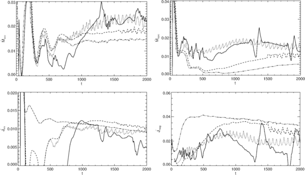
Figure 23. Effect of the magnetic diffusivity scale height. Shown is the evolution of the accretion and ejection rate  (top), and the evolution of the kinetic and magnetic angular momentum flux
  (bottom), for simulations applying a different diffusive scale height Hη = 0.1 (solid line), 0.2 (dotted line), 0.3 (dashed line), and 0.4 (dot-dashed line).
Download figure:
Standard image High-resolution image
For increasing scale height the accretion rate and ejection rate decrease, confirming the correlation derived above between the increasing magnitude of diffusivity and decreasing mass fluxes. In other words, an increasing diffusivity scale height simply corresponds to a higher diffusivity with the consequences as discussed above. Interestingly, all our simulations for different diffusivity scale heights converge to the same kinetic angular momentum flux in the outflow. On the other hand, we find a trend of decreasing magnetic angular momentum flux with decreasing diffusivity scale height.
5. COMPARISON WITH PREVIOUS NUMERICAL STUDIES
In this section we highlight some of our results, discussing them in the context of numerical studies published previously. Our main goal was to perform a consistent parameter study to investigate a variety of physical effects involved in jet launching by using one code with one numerical setup. Only this allows us to disentangle the leading effects involved in jet launching without the uncertainty introduced by interpreting results obtained with different codes (VAC, PLUTO, and FLASH) or setups.
We first stress the point that we apply a well defined, fixed-in-time magnetic diffusivity distribution. The magnetic diffusivity is a leading parameter which influences the whole disk–jet evolution (Zanni et al. 2007). Previous simulations (Casse & Keppens 2002; Zanni et al. 2007; Tzeferacos et al. 2009; Murphy et al. 2010) have applied a diffusivity evolving in time. This might be considered as more advanced; however, these authors do not provide details about time evolution of the diffusivity, thus introducing some level of uncertainty. Here, we have demonstrated how diffusion and advection of magnetic flux does change the disk Alfvén speed (and thus the magnetic diffusivity if a time-dependent η(t) ∼ vA(t) is applied) by a factor of 10. On the other hand, by applying different strength and scale height for the diffusivity we investigate the interrelation between magnetic diffusivity and the accretion and ejection mass fluxes.
Similarly, we provide information about the spatiotemporal evolution of the magnetization (or plasma-β in our case). Tzeferacos et al. (2009) have published a magnetization study, but on a smaller grid and for substantially shorter dynamical evolution. In our paper, we show in particular how the magnetization profile flares over thousands of dynamical timescales (Figure 17). Thus, along with the evolving outflow, the magnetization above the disk surface is substantially lower compared to the initial condition.
We obtain jet velocities which seem to be smaller compared to previously published values. For example, Zanni et al. (2007) detect asymptotic velocities of 1.5–1.8 times the footpoint Keplerian speed for the field lines crossing the upper boundary. Simulations of jet formation from a fixed-in-time disk surface boundary (see, e.g., Ouyed & Pudritz 1997; Fendt & Čemeljić 2002) give similar values. In contrast, we report lower velocities of about 0.8 times the Keplerian speed at the inner disk radius. Note, however, that our values result from a differently defined measure of the jet velocity. We suggest that this mass-flux weighted asymptotic speed—the average velocity of the bulk mass flux—is more applicable to observations. The maximum jet velocities we observe in our simulations are higher and also up to 1.8 times the Keplerian speed at the inner disk radius, which is consistent with previous studies. We explicitly consider the jet rotation in our simulations, a topic which has not been treated in previous launching simulations.
We quantify the jet collimation degree by the directed mass fluxes. For the jet opening angle we find somewhat larger values than in previous studies. We suppose that this results from the modified outflow condition we have applied as we have seen that the original outflow condition lead to smaller opening angles.
We have run long-lasting simulations of up to 5000 dynamical timescales ti = ri/vK, i. This allows us to reach a quasi-steady-state situation of the simulation, but also to investigate the evolution beyond. We find a slight but persistent change in the inflow–outflow dynamics on these very long timescales, such that the accretion rate slightly decreases. The main reason for this we see in the decrease of the disk mass for such long timescales. However, the effect has a direct astrophysical application as it may be applied to the long-term evolution of classical T Tauri stars when the disk accretion in fact weakens after some 106 years. Clearly, our simulation covers a much smaller period of time, namely, about 25 years only (for the scaling applied in this paper). However, we may mimic the long-term evolution by providing a limited-mass reservoir only. We note that previous simulations were substantially shorter, lasting until 400 dynamical time steps ti = ri/vK, i (Zanni et al. 2007; Tzeferacos et al. 2009) or 30 inner disk rotations (Casse & Keppens 2004; Meliani et al. 2006). An exception is the simulation by Murphy et al. (2010) lasting for more than 900 inner disk orbits. That paper focuses, however, on the launching physics and does not show the large-scale evolution of the outflow.
Together with the long-time evolution, we have also have applied a large grid size. Compared to Tzeferacos et al. (2009) who investigated how magnetization affects launching by using a 40 × 120 ri grid, our grid was about double the size. Murphy et al. (2010) concentrated on the launching process of weakly magnetized disks and displayed only results on 40 × 40 ri images (which are a subset of a 280 × 840 ri). For YSO, our grid extension corresponds to about 28 AU along the jet, well into the observable region. We note that we have applied an equidistant grid for the magnetically diffusive disk area which is consistent with the PLUTO code requirements. This is different to Murphy et al. (2010) who attached a scaled grid for the diffusive outer disk.
6. CONCLUSIONS
We have presented results of MHD simulations investigating the launching of jets and outflows from a magnetically diffusive disk in Keplerian rotation. The time evolution of the accretion disk structure is self-consistently taken into account. The simulations are performed in axisymmetry applying the MHD code PLUTO. The main goal of our simulations was to study how magnetic diffusivity (its magnitude and distribution) and magnetization affect the disk and outflow properties, such as mass and angular momentum fluxes, jet collimation, or jet radius.
Our grids extend to (96 × 288) inner disk radii with a resolution of (0.064 × 0.066), respectively (50 × 180) inner disk radii with a higher resolution of (0.025 × 0.025). An internal boundary (sink) is placed close to the origin absorbing the accreted mass and angular momentum.
We have prescribed a magnetic diffusivity in the disk based on an α-prescription. One of our parameters was the scale height of the magnetic diffusivity with the option to have it higher than the thermal scale height. This can be justified considering that it is the turbulent disk material which is loaded into the outflow, and that the turbulence pattern is swept along with the disk wind until it decays. We have investigated disks carrying a magnetic flux corresponding to an initial plasma-β ranging from 10 to 5000 at the inner disk radius.
As a general result we observe a continuous and robust outflow launched from the inner part of the disk, expanding into a collimated jet and is accelerated to superfast-magnetosonic speed. The key results of our simulations can be summarized as follows.
- 1.Concerning the acceleration of the outflows, our simulations confirm that the magnetocentrifugal acceleration mechanism is most efficient in the low plasma-β regime, while for weak magnetic fields the toroidal magnetic pressure gradient drives the ejected material.We also confirm that the magnetocentrifugal mechanism depends on the mass load in the outflow, as this mechanism works more efficiently for outflows with low-mass fluxes. However, compared to the magnetic-pressure-driven outflows, jets in the magnetocentrifugal acceleration regime have usually higher mass fluxes.In our simulations with very high plasma-β we detect a highly unsteady behavior.
- 2.Efficient magnetocentrifugal driving which can accelerate jets to high kinetic energy relies on a strong coupling between magnetic field and the rotating disk, thus on a low diffusivity. We find that it is the poloidal diffusivity ηp which mainly affects the driving of the outflow. However, besides the coupling needed for acceleration, the launching of material also depends on diffusivity. With increasing ηp, the mass fluxes (both the accretion rate and the ejection rate) decrease. Subsequently, the higher ejection rates result in a lower asymptotic outflow velocities.
- 3.We measure typical outflow velocities in the range of 0.3–0.8 times the inner disk rotational velocity with the tendency that the mass fluxes obtained in magnetocentrifugally driven outflow are substantially higher. Here, we confirm the clear (inverse) correlation between jet velocity and mass load, as is well known from the literature. Note that we have applied a mass-flux-weighted jet velocity which we find more applicable to the observations. For the bulk mass flux we find lower velocities compared to other papers, which are mostly dealing with the maximum speed obtained in the simulation. Our maximum velocities are similar. The relatively high speed of the outflows with low Poynting flux which are driven by poloidal pressure gradient is unclear.We find that the toroidal diffusivity affects the outflow rotation—a small toroidal diffusivity implies a larger jet rotational velocity. This has not been shown before in simulations.
- 4.We do not find a clear correlation between the outflow collimation and the magnetic field strength. Also weakly magnetized outflows, which are driven by the magnetic pressure gradient, and which we find to be quite unsteady, show a high degree of collimation. The question of collimation for the weakly magnetized outflows is not answered.We find that for outflows within the magnetocentrifugal-driving regime, the flows ejected from weakly diffusive disks are only weakly collimated. Similarly, their jet radius (here defined as mass-flux-weighted radius) is larger in the case of a lower poloidal magnetic diffusivity.Following the magnetic flux surface along the bulk mass flux from the asymptotic regime to the launching area, we can define the launching area of the outflow. We find a size of the launching area from which the bulk of the mass flux originates in the range between 3 and 8 inner disk radii or about 0.4 AU.
- 5.Depending on the strength of magnetic diffusivity, the disk–jet structure may evolve into a steady state. We find that the cases with the strong field with βi ∼ 10 and poloidal diffusivity ηp, i ⩾ 0.03 will reach a quasi-steady state, confirming the literature.
- 6.The magnetic flux profile along the disk is subject to advection and diffusion. We find that the magnetization (or plasma-β) of disk and outflow may therefore substantially change during the time evolution. We have observed that the initial disk magnetization may change by a factor of 100. This may have a severe impact on the launching process and the formation of the outflow in the sense that a rather highly magnetized disk may evolve into a weakly magnetized disk which cannot drive strong outflows. This issue has not been discussed before in the literature.
- 7.For very long timescales the accretion disk changes its internal dynamics, as due to outflow ejection and disk accretion the disk mass decreases. As a consequence, the accretion and ejection rates slightly decrease. In order to compensate for this effect, we have applied a large outer disk radius providing a large-mass reservoir for the inner jet-launching disk.
- 8.For our simulations, we find that 10%–50% of the accreting plasma can be diverted into the outflow. For (1) less diffusive disks, (2) a strong magnetic field, (3) a low poloidal diffusivity, or (4) a lower numerical diffusivity (resolution), the mass loading into the outflow is increased—resulting in more massive jets. We interpret the physical reason for this to be the result of the more efficient extraction of angular momentum from the disk, due to the stronger matter–field coupling. Note that we do not consider in our simulations viscosity or the wealth of thermal effects which play an essential role for launching (Casse & Ferreira 2000).
- 9.We found that jets launched in a setup with smaller diffusive scale height are more perturbed. The same effect is seen in outflows launched from disks with weaker diffusivity.
- 10.We finally remark that it is essential to perform long-term simulations covering thousands of rotational periods in order to find a steady-state situation of the accretion–ejection dynamics. Our simulations run for 5000 dynamical timesteps, corresponding to about 800 revolutions at the inner disk radius as adopted in our reference run. We should, however, note that this run time corresponds to only 25 years of young stellar evolution for a solar mass star and an inner disk radius of 0.1 AU. However, our simulations allow us to mimic nature such that we can follow a slight trend in the disk–jet evolution due to the limited-mass reservoir.
In summary, we confirm the hypothesis that efficient magnetocentrifugal jet driving requires a strong magnetic flux (i.e., a low plasma-β), together with a large enough magnetic torque in order to produce a powerful jet. In addition, the magnitude of (turbulent) magnetic diffusivity plays the major role in the ejection efficiency, while the anisotropy in the diffusivity mainly affects the jet rotation. Both results imply that the structure of the asymptotic jet is indeed governed by the properties of the accretion disk, here parameterized by the magnetization and magnetic diffusivity. The mass ejection-to-accretion ratio along with the momentum and energy transfer rates from inflow to outflow are essential properties for any feedback mechanism in star or galaxy formation scenarios and can only be derived from simulations resolving the inner region of the jet-launching accretion disk.
We thank Andrea Mignone and the PLUTO team for the opportunity to use their code. We acknowledge helpful and constructive criticism by two referees, which has improved the presentation of the paper. S.S. acknowledges the warm hospitality by the Max Planck Institute for Astronomy. All simulations were performed on the THEO cluster of the Max Planck Institute for Astronomy. This work was financed partly by a scholarship of the Ministry of Science, Research, and Technology of Iran, and by the SFB 881 of the German science foundation DFG.
APPENDIX A: UNITS AND NORMALIZATION
We normalize all variables, namely, r, ρ, v, and B to their fiducial values at the inner disk radius. We have adopted the following typical number values for a YSO of M = 1 M☉ and an AGN of M = 108 M☉. A change in one of the system parameters accordingly changes the scaling of our simulation results which can thus be applied for a variety of jet sources. The inner disk radius ri is usually assumed to be a few radii of the central object,
where RS = 2GM/c2 is the Schwarzschild radius of the central black hole. The inner disk radius is usually assumed to be located at the marginally stable orbit at 3 RS. Since we apply the non-relativistic version of the PLUTO code, we cannot treat any relativistic effects. We therefore apply a scaling of ri ≃ 10 RS. For simplicity and convenient comparison with the previous literature we apply ri = 0.1 AU for most comparisons concerning stellar sources. The orbital velocity at the inner disk radius is
For a ri = 0.1 AU distance from a YSO, the orbital speed is vk, i = 94 km s−1. The mass accretion rate is a parameter which is in principle accessible by observation. Subject to the disk model applied, the observed disk luminosity can be related to an accretion rate. For a YSO, the accretion rate is typically of the order of  , providing a normalization of the density ρi with
  . Applying a length scale ri = 0.1 AU and a velocity scale vk, i = 94 km s−1, we obtain
Normalized value of the magnetic field is obtained by considering the plasma-β and the field strength at the equator at the inner radius  ,
,
APPENDIX B: A MODIFIED RADIAL OUTFLOW BOUNDARY CONDITION
An essential point of our setup is to impose an outflow boundary at the outer part of the domain in the r-direction avoiding artificial collimation. We have implemented a current-free outflow boundary condition which prevents spurious collimation by Lorentz forces and which has been thoroughly tested in our previous papers (Porth & Fendt 2010; Porth et al. 2011; Vaidya et al. 2011). The boundary condition considers a vanishing toroidal electric current density in the ghost cells. Therefore, the Lorentz force component perpendicular to the grid boundary vanishes. The boundary constraints are applied on the poloidal and toroidal component of the electric current density, jr = −∂zBϕ, jz = r−1∂rrBϕ, and jϕ = ∂zBr − ∂rBz, respectively.
In principle, this is considered for the grid ghost cells (iend, j) adjunct to the domain boundary at (iend + 1, j) (see the Section 3.1.1 in Porth & Fendt 2010). The transverse Bt(iend, j + 1/2) and normal Bn(iend + 1/2, j), Bn(iend + 1/2, j + 1) magnetic field components in the domain, together with the transverse field component Bt(iend + 1, j + 1/2) of the first ghost zone, constitute a toroidal corner-centered electric current Iϕ(iend + 1/2, j + 1/2). With that a constraint for a current-free Iϕ = 0 boundary condition can been implemented numerically,
Footnotes
- 5
In PLUTO the magnetic field is normalized considering 4π = 1.
- 6
Although previous publications have applied a stretched grid also for the part of the domain enclosing the disk structure (see, e.g., Murphy et al. 2010), we note that up to the latest version of the code, PLUTO 3.1., the treatment of magnetic diffusivity is limited to equidistant grids (see the PLUTO user manual).
- 7
zs is defined corresponding to the resolution, at least four cells are taken as a sink height in any run.
- 8
We will later show that we do not resolve the MRI with the numerical resolution applied in our disk–jet setup (see Section 4).
- 9
The ηϕϕ effectively governs the diffusion of the poloidal magnetic field, while the ηrr and ηzz govern the diffusion of the toroidal magnetic field.
- 10
We remark that in previous simulations which evolve η in time, only the initial diffusivity distribution was provided, but not its temporal evolution, and, thus, the magnetic diffusivity distribution which is actually involved in producing the outflow (see, e.g., Zanni et al. 2007; Tzeferacos et al. 2009; Murphy et al. 2010). See also our numerical example below.
- 11
Averaging in time is applied for all flux evolutions.
- 12
For high plasma-β (cases 9 and 10), the mass fluxes evolution looks strongly fluctuating and is therefore omitted.
- 13
We cannot compare cases 1 and 4 or 5 and 4 directly, as, due to their different poloidal diffusivity, these outflows have different mass fluxes.
- 14
For simulations with higher resolution (case 6 and case 7), we adopt a smaller physical grid size with rout = 50, so we cannot compare the jet radius properly.