


ABSTRACT
We present Spitzer Space Telescope 5–36 μm mapping observations toward the southeastern lobe of the young protostellar outflow HH 211. The southeastern terminal shock of the outflow shows a rich mid-infrared spectrum including molecular emission lines from OH, H2O, HCO+, CO2, H2, and HD. The spectrum also shows a rising infrared continuum toward 5 μm, which we interpret as unresolved emission lines from highly excited rotational levels of the CO v = 1–0 fundamental band. This interpretation is supported by a strong excess flux observed in the Spitzer/IRAC 4–5 μm channel 2 image compared to the other IRAC channels. The extremely high critical densities of the CO v = 1–0 ro-vibrational lines and a comparison to H2 and CO excitation models suggest jet densities larger than 106 cm−3 in the terminal shock. We also observed the southeastern terminal outflow shock with the Submillimeter Array and detected pure rotational emission from CO 2–1, HCO+ 3–2, and HCN 3–2. The rotationally excited CO traces the collimated outflow backbone as well as the terminal shock. HCN traces individual dense knots along the outflow and in the terminal shock, whereas HCO+ solely appears in the terminal shock. The unique combination of our mid-infrared and submillimeter observations with previously published near-infrared observations allow us to study the interaction of one of the youngest known protostellar outflows with its surrounding molecular cloud. Our results help us to understand the nature of some of the so-called green fuzzies (Extended Green Objects), and elucidate the physical conditions that cause high OH excitation and affect the chemical OH/H2O balance in protostellar outflows and young stellar objects. In an appendix to this paper, we summarize our Spitzer follow-up survey of protostellar outflow shocks to find further examples of highly excited OH occurring together with H2O and H2.
Export citation and abstract BibTeX RIS
1. INTRODUCTION
Shocks driven by a variety of sources strongly influence the chemistry and physics in the interstellar medium: they accelerate, heat, and compress interstellar gas, erode dust grains, and drive interstellar chemistry. The high sensitivity and mid-IR spectral mapping capabilities of the Spitzer Space Telescope, now powerfully complemented at longer wavelengths by the Herschel Space Observatory, make it possible to study many of the underlying physical and chemical processes. The large number of cooling lines from rotationally excited molecules in combination with the atomic fine-structure transitions can be used as sensitive diagnostics to analyze the shock chemistry and excitation conditions.
Bipolar outflows associated with accretion processes in young stellar objects (YSOs) are well-known tracers of star formation activity. Herbig–Haro (HH) objects, small emission nebulae found in star-forming regions originally studied in the optical in the 1950s by G. Herbig and G. Haro, are now recognized as manifestations of outflow shock activity (Reipurth & Bally 2001). However, the youngest outflows are often optically invisible since they are still obscured by the dense star-forming cloud. Shocks occur at the point where the supersonic jet flow hits the ambient medium from which the star was forming. In addition, many young jets show characteristic knots or "molecular bullets" of high density along the jet axis (see, e.g., Reipurth & Bally 2001). The study of the youngest protostellar outflows that are just emerging from the protostellar envelope offers not only insights into their own unique properties but also the connection with the protostellar disk accretion process as well as the physics and chemistry of star-forming regions.
In this paper, we present an observational follow-up study of the very young protostellar outflow HH 211. In our previous Spitzer observations, we detected a unique sequence of superthermal OH emission lines in the southeastern (SE) terminal shock of HH 211 (Tappe et al. 2008). Our main goal is to disentangle the complex chemical and physical spatial structure of the SE outflow lobe of HH 211, which is an important prerequisite for a meaningful theoretical discussion. In Section 2, we describe the observations and data reduction. Section 3 presents the results of our extended Spitzer Infrared Spectrograph (IRS) mapping observations as well as complementary Submillimeter Array (SMA) observations toward the SE terminal shock. Finally, in Sections 4 and 5, we analyze and discuss the unique spectral features of HH 211, including a likely detection of CO v = 1–0 fundamental band emission as well as the implications for the nature of Extended Green Objects (EGOs) and the structure of young protostellar outflows.
2. OBSERVATIONS AND DATA REDUCTION
2.1. Spitzer
We observed the protostellar outflow HH 211 with Spitzer/IRS (Houck et al. 2004) on 2007 March 12, 2008 October 9, and 2009 March 7. We mapped the complete outflow including the region ahead of the SE terminal shock using the IRS short–high (SH, 9.9–19.6 μm) and long–high (LH, 18.7–37.2 μm) modules. We also obtained short–low module observations (SL2/SL1, 5.2–8.7/7.4–14.5 μm) of the SE terminal shock and the region ahead of it complementary to the existing Spitzer archival data covering the rest of the outflow. Finally, we combined our mapping observations with the single pointing observation toward the HH 211 SE terminal shock taken on 2008 October 6 (PI: B. Nisini, PID 50364, Spitzer data archive) to further improve the signal-to-noise ratio (S/N). We observed the protostellar outflows HH 111, HH 212, HH 240, HH 2, and NGC 2264 G with Spitzer/IRS (Houck et al. 2004) between 2008 October 10 and 2009 April 13. We mapped selected outflow regions using the IRS SL, SH, and LH modules. The nominal spectral resolution is R = 64–128 as a function of wavelength for the low-resolution and R = 600 for the high-resolution IRS modules. We also obtained Infrared Array Camera (IRAC; Fazio et al. 2004) image mosaics from the Spitzer data archive.
We performed the IRS data reduction consisting of background subtraction using off-source slit positions, masking of bad pixels, extracting the spectra, and generating the spectral line maps with CUBISM version 1.7 (Smith et al. 2007a). The individual steps of our data reduction are as follows.
- 1.Start with the basic calibrated data as provided by the Spitzer/IRS pipeline.
- 2.Import observations taken sequentially in time with each IRS module into a CUBISM project.
- 3.Select and subtract an average background in CUBISM by using all slit positions devoid of source emission.
- 4.Identify and exclude remaining bad pixels using CUBISM's automated statistical algorithms.
- 5.Build the data cube using CUBISM's slit loss correction function (SLCF) for extended sources.
- 6.
- 7.

Figure 1. HH 211 blueshifted SE outflow: Spitzer/IRS merged spectrum of the terminal shock. The individual spectrograph modules are indicated at the bottom. All spectral lines discernible at this plotting scale are labeled. Pure rotational H2O lines are marked with an asterisk. Figure 2 shows a detailed view of the 10–15 μm region. The dashed box in Figure 3 shows the extraction region of this IRS spectrum.
Download figure:
Standard image High-resolution imageWe applied scaling factors to seamlessly merge the spectra from the LH and the SL modules with the SH module to produce combined 5–36 μm spectra. The order mismatches are due to calibration issues inherent to slit spectroscopy of inhomogeneous, extended sources, which are partially corrected by CUBISM's SLCF. To address the remaining mismatches in a consistent way, we scaled the LH spectrum so that the continuum flux and the adjacent OH spectral lines in the two high-resolution modules match. The SL module spectra were scaled to match the H2 S(2) 12.28 μm line flux in the SL2 and the SH module. The mismatches between the different modules that we corrected in this way were less than 30%. In the case of HH 211, for example, the scaling factors applied to the LH and SL modules were 1.28 and 1.15, respectively.
2.2. SMA
Observations toward the SE terminal shock of the HH 211 jet were carried out with the SMA on 2008 November 9 and 16 in the compact configuration. During the first track, the main aim was to observe the HCO+ 3–2 line at 267.5 GHz and the nearby HCN 3–2 line at 265.9 GHz while the second track contained the CO 2–1 line at 230.5 GHz for reference. During the first track, the zenith opacity was excellent with τ225 GHz ∼ 0.05. During the second track, conditions were foggy with a higher opacity of τ225 GHz ∼ 0.2–0.3 during the first few hours of the track and a stable value of τ225 GHz ∼ 0.1 later on. Phases were very stable during the whole track. The correlator configuration was set to a frequency resolution of 0.4 MHz across the 2 GHz wide band. This resulted in a velocity resolution of ∼0.5 km s−1 at the observed frequencies. The primary beam sizes for HCO+ 3–2 and HCN 3–2 are ∼47'' and ∼54'' for CO.
We have used the MIR software package, with quasars 3C454.3, 3C84, and 3C111 as passband calibrators, 3C84 and 3C111 as gain calibrators, and Callisto and Titan as flux calibrators. The resulting estimated absolute flux uncertainty is ∼20%. The calibrated visibilities were subsequently processed with the MIRIAD software package. The resulting synthesized beam sizes are 2 3 × 19, P.A. −56° for HCN and HCO+, and 25 × 20, P.A. −47° for CO. The rms noise level in the CO data is 37 mJy beam−1 at a velocity resolution of 1 km s−1 and 23 mJy beam−1 in both HCN and HCO+, again at velocity resolutions of 1 km s−1.
3. RESULTS
3.1. Spitzer/IRS
Figures 1 and 2 show the Spitzer/IRS spectrum extracted from a small region near the center of the terminal shock of HH 211 (see the dashed box in Figure 3). The main features of the spectrum, in particular the unique sequence of superthermal OH rotational lines, have been discussed earlier by Tappe et al. (2008). Here, we focus on the aspects of the spectrum that relate to the spatial structure and excitation of the gas in the SE terminal shock as well as the underlying outflow jet in the SE lobe of HH 211. In addition to the spectral features discussed by Tappe et al. (2008), we now detect 5σ emission lines of the ν2 fundamental vibrational band Q-branches of HCO+ at 12.07 μm and CO2 at 14.97 μm in the SE terminal shock. These weak lines were not seen earlier due to a lower S/N. Another notable and unusual feature of the terminal shock spectrum is the rising infrared continuum emission toward 5 μm. We discuss this aspect of the spectrum in detail in Section 4.1.1.
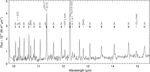
Figure 2. HH 211 blueshifted SE outflow: IRS spectrum of the terminal shock (detail from Figure 1).
Download figure:
Standard image High-resolution image
Figure 3. HH 211 blueshifted SE outflow: Spitzer emission line maps (this work, white contour lines) overlaid on a near-infrared H2 1–0 S(1) 2.12 μm image (Hirano et al. 2006). Top panel: sum of high-J OH lines in the 10–17 μm region. Middle panel: [Fe ii] 5.34 μm from this work and optical Hα from Walawender et al. (2006). Bottom panel: 5.3 μm continuum excluding line emission. The small dashed box marks the extraction region of the IRS spectrum in Figure 1. FWHM beam sizes are indicated as circles in the bottom right corner. Boxes indicate the Spitzer/IRS module pixel size and orientation. The white arrow marks the extent and direction of the dense, collimated inner jet of HH 211 (Hirano et al. 2006).
Download figure:
Standard image High-resolution imageFigure 3 shows a selection of emission line contour maps generated with CUBISM from our Spitzer/IRS mapping observations of the SE outflow lobe (see Section 2). The contour maps are plotted on a recent near-infrared H2 1–0 S(1) 2.12 μm image of HH 211 (Hirano et al. 2006). The spatial resolution of the Spitzer/IRS observations at the shortest wavelength of the SL module at 5.3 μm is good enough to partially resolve the structure of the terminal shock as seen in the near-IR H2 image (cf. FWHM beam sizes in Figure 3, middle and bottom panels).
In the top panel of Figure 3, we show the integrated emission from the superthermal OH with nearly complete coverage including the region ahead of the shock as well as improved S/N compared to our earlier work (Tappe et al. 2008). We can now clearly state that there is no discernible superthermal OH emission ahead of the terminal shock as traced by vibrationally excited H2. Instead, the OH emission maximum seems to be just ahead of the Hα, [Fe ii] 5.34 μm, and H2 1–0 S(1) 2.12 μm emission maxima (see the middle panel in Figure 3). Furthermore, we note that the observed infrared 5.3 μm continuum (bottom panel of Figure 3) is spatially extended along the central jet axis and has a weak maximum coinciding with the secondary H2 2.12 μm maximum at the very head of the terminal shock. We discuss this interesting fact in more detail in Section 5.
3.2. Spitzer/IRAC
The top four panels in Figure 4 show archival Spitzer/IRAC images of the SE, blueshifted outflow lobe of HH 211 (pipeline S18.18, observation program 50596 by G. Rieke, 2009 March) in comparison to H2 2.12 μm contours (Hirano et al. 2006). The nominal IRAC detector pixel size is 12 in all channels, and the pipeline product images are sampled to a pixel size of 06. The rising background in channels 3 and 4 is due to emission from polycyclic aromatic hydrocarbons (PAHs) at 6.2 and 7–9 μm. We measured the IRAC fluxes of the terminal shock by performing simple aperture photometry with a source annulus diameter of 12'' centered at 3h43m59 45, 32°00'360 (J2000). The flux shows a distinct peak in IRAC channel 2, with background-subtracted fluxes for channels 1, 2, 3, and 4 of 5.2, 26.0, 13.0, and 9.6 mJy, respectively.
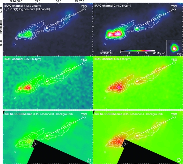
Figure 4. HH 211 blueshifted SE outflow IRAC images (top four panels, IRAC channels 1–4) compared to IRS SL CUBISM channel maps interpolated to the IRAC pixel size (bottom two panels, corresponding to IRAC channels 3 and 4) and H2 2.12 μm contours (Hirano et al. 2006). The original IRS SL pixel size and the approximate FWHM beam size are indicated in the bottom two panels (bottom right corner). A representative IRAC point-spread function (PSF) from a star located close to HH 211 is shown for IRAC channel 2. All panels have the same logarithmic color scale shown in the top right panel.
Download figure:
Standard image High-resolution imageWe also note that the spatial flux distribution within the terminal shock is notably different in channel 2. The peak flux is located in an unresolved, point-like source at the head of the terminal shock. In the other channels, the IRAC flux peak coincides with the H2 1–0 S(1) 2.12 μm flux maximum, which is expected since the IRS mid-infrared spectrum of HH 211 is dominated by H2 pure rotational lines. This difference suggests that another atomic or molecular species is responsible for the flux peak in IRAC channel 2.
To further analyze the nature of the channel 2 flux, we can use our Spitzer/IRS SL mapping data to generate IRAC channel 3 and 4 maps with CUBISM. These maps are shown in the bottom two panels of Figure 4. We have added a constant background flux to those images to account for the fact that the surrounding background emission was previously subtracted in the IRS maps. Doing the same kind of aperture photometry on the CUBISM generated maps yields background-subtracted fluxes of 8.9 and 8.5 mJy for channels 3 and 4. This includes an approximation for a few missing pixels at the edge of the aperture due to incomplete IRS coverage (<5% of the total flux).
The CUBISM-predicted channel 4 flux of 8.5 mJy is about 10% below the measured IRAC channel 4 value, which is within the expected uncertainty due to the IRS and IRAC absolute flux calibration accuracy. However, the predicted channel 3 flux is about 30% below the measured IRAC flux. Even when including an approximate upper limit flux estimate for the H2 S(8) pure rotational line at 5.05 μm, which is not covered by the IRS spectral range, the flux is still at least 20% below the observed IRAC flux. This "missing" flux must come from emission in the 5.0–5.3 μm range, which is not covered by the IRS but within the IRAC channel 3 bandpass. We hypothesize that the missing flux in channel 3 as well as part of the channel 2 emission are due to CO v = 1–0 fundamental band lines. We discuss the reasoning behind this hypothesis in Section 4.1.1.
3.3. SMA
Figure 5 shows our SMA CO 2–1, HCO+ 3–2, and HCN 3–2 data. We chose the velocity intervals and color coding to highlight the different jet structures and overlaid the HCO+ and HCN as well as the H2 1–0 S(1) data contours for comparison. Despite the decreasing sensitivity beyond the FWHM of the SMA primary beam, our observations trace the CO jet all the way to the YSO. We detect several HCN knots that coincide with H2 knots visible in the H2 1–0 S(1) 2.12 μm image (see white contours in Figure 5). The terminal shock also shows HCN as well as HCO+ emission coinciding with maxima of vibrationally excited H2 emission. We note that HCN and HCO+ trace different regions of the terminal shock. The peak of the HCO+ emission coincides with the primary and secondary peaks of H2 1–0 S(1), whereas the HCN peak coincides with a small H2 protrusion upstream of the main maxima. This protrusion is also visible in our CO 2–1 data.
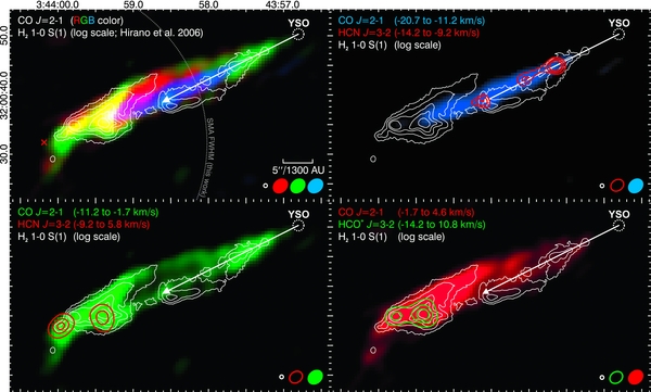
Figure 5. HH 211 blueshifted SE outflow: comparison of SMA emission line maps (this work) with near-infrared H2 1–0 S(1) 2.12 μm observations (Hirano et al. 2006). The respective beam sizes are indicated in the bottom right corner of each panel. Top left: three-color RGB CO image of different radial velocity channels, which are individually displayed in the other three panels. Top right: blue CO velocity channel and inner jet HCN knots. Bottom left: green CO velocity channel and terminal shock HCN knots. Bottom right: red CO velocity channel and HCO+ knots. The SMA pointing and FWHM are indicated by a red cross and dotted circle in the top left panel. The systemic LSR velocity is +9.2 km s−1 (Lee et al. 2010).
Download figure:
Standard image High-resolution imageNote that the CO 2–1, HCO+ 3–2, and HCN 3–2 lines have different critical densities but similar upper energy levels between 15 and 26 K. The CO 2–1 line has the lowest critical density of ∼7 × 103 cm−3, whereas HCN and HCO+ 3–2 have critical densities ∼8 × 107 cm−3 and ∼4 × 106 cm−3, respectively (Tielens 2005). Lines with high critical densities cause an observational bias favoring regions with gas densities similar to the respective critical density. In this case, we expect that HCN and HCO+ trace the denser regions of the CO jet. HCO+ is also a tracer of ionization, whereas HCN predominantly traces neutral or low-ionization gas in comparison. We further discuss the HCO+ and HCN emission in Section 5.2.
4. ANALYSIS
4.1. Evidence for CO Fundamental Band Emission
4.1.1. Rising Infrared Continuum toward 5 μm and CO Model Spectrum
Figure 6 compares the observed Spitzer/IRS SL spectrum integrated over the entire HH 211 SE terminal shock area with a local thermodynamic equilibrium (LTE) CO model spectrum at the resolution of the Spitzer/IRS SL module, R = 90, and with plausible parameters for CO column density and temperature (see the legend of Figure 6). The CO model spectra were generated with the Spectrafactory tool5 (see Cami et al. 2010 for further details on the model) using the Goorvitch CO line list, which contains all the rotation-vibration transitions of the fundamental, first, and second overtone bands up to v = 20 and J = 149 of the CO X 1Σ+ state (Goorvitch 1994). We also show a CO model spectrum at a higher resolution of R = 2000 to illustrate the individual ro-vibrational lines as well as the four IRAC channel bandpasses. We scaled the CO model spectrum to reproduce the estimated, dereddened IRAC channel 2 excess flux that we attribute to CO (green bar in Figure 6; see further analysis below). The scaling of the LTE spectrum is necessary because the very high critical densities of the ro-vibrational CO v = 1–0 fundamental band transitions cause a departure from LTE energy level populations at the expected densities in HH 211. For that reason, we caution that the temperature and the column density assumed for the LTE CO model represent only a rough but physically plausible estimate until further revised by a non-LTE CO model (see Section 4.1.2 for further discussion). Nevertheless, we expect that the relative ro-vibrational line intensities within the CO v = 1–0 fundamental band are approximately correct and sufficiently accurate to demonstrate that the rising pseudo-continuum toward 5 μm can plausibly be attributed to CO.

Figure 6. HH 211 terminal shock: observed Spitzer/IRS SL spectrum integrated over the entire SE terminal shock area and simulated Spectrafactory LTE CO spectrum (see the plot legend and Section 4.1.1 for further details). The near-IR spectra that we used to derive the CO overtone band upper limit were provided by O'Connell et al. (2005) and Caratti o Garatti et al. (2006).
Download figure:
Standard image High-resolution imageTo obtain an estimate of the channel 2 excess flux beyond pure H2 emission, we subtracted a scaled IRAC channel 1 image from channel 2. The channel 1 scale factor of 2.4 is a fairly typical value for warm H2 (cf. Neufeld & Yuan 2008, Figures 1 and 7) and in the case of HH 211 subtracts most of the H2 emission along the outflow. The resulting H2-subtracted IRAC image is shown in the top panel of Figure 7. For comparison, we show the CO 2–1 SMA jet backbone and Spitzer 5.3 μm continuum contours (cf. Figures 3 and 5) as well as the optical Hα contours from Walawender et al. (2006). It is striking that the estimated channel 2 excess follows the observed Spitzer 5.3 μm continuum flux very closely. Furthermore, the channel 2 excess/5.3 μm continuum seems to be a spatial continuation of the SMA-observed CO jet backbone with the Hα emission located at the transition point between the two. These are further indications that the IRAC excess flux is indeed due to CO fundamental band emission. The prerequisites for CO fundamental band emission, high density CO gas and suitable excitation conditions, are both met in the SE terminal shock of HH 211.

Figure 7. HH 211 blueshifted SE outflow: estimate of H2-subtracted IRAC channel 2 excess emission (top panel) and 2.14 μm narrowband continuum contours from Eislöffel et al. (2003) overlaid on H2 1–0 S(1) image from Hirano et al. (2006) (bottom panel). Contours are explained and approximate FWHM beam sizes are indicated in the bottom right in each panel. Note that we corrected the astrometry of the 2.14 μm narrowband continuum image provided by Eislöffel et al. (2003) and that the observed flux is most likely due to H2 1–0 S(1) 2.12 μm flux leaking into the continuum filter (see Section 4.1.1 for a discussion).
Download figure:
Standard image High-resolution imageWe can exclude that the excess flux is due to continuum emission from hot dust grains. Dust emission with a flux maximum shortward of 5 μm would be from hot dust and would show a strong silicate feature in emission near 10 μm. This is not observed in our Spitzer/IRS spectrum. Instead, the dust continuum peaks longward of 20 μm and can be fitted by thermal dust emission at modified blackbody temperatures of 30–170 K (Tappe et al. 2008). The H i Brα line could be another potential contribution to IRAC channel 2 emission. However, only a small area of the HH 211 SE terminal shock shows H i Hα emission and it does not spatially correlate with the IRAC channel 2 excess emission (see Figure 7, top panel).
It was previously suggested that the observed HH 211 2.14 μm near-infrared continuum, see the solid white contours displayed in the bottom panel of Figure 7, is partially due to scattered light that originates close to the protostar and escapes along the outflow path (Eislöffel et al. 2003; O'Connell et al. 2005). O'Connell et al. (2005) pointed out that the near-infrared emission nearer the YSO source traces predominantly scattered light while the emission further out mostly traces compact, H2 line-emission features.
We can measure the near-infrared continuum flux from a 2.14 μm narrowband continuum filter image provided by Eislöffel et al. (2003). We estimate an upper limit of 1.5 × 10⁻¹⁷ W m−2 for the dereddened 2.14 μm continuum flux of the SE terminal shock of HH 211. This upper limit includes a 35% flux uncertainty due to the calibration and low S/N. For the dereddening, we assumed a visual extinction toward the terminal shock of 10 mag and the RV = 3.1 extinction law by Weingartner & Draine (2001) and Draine (2003).
It is very likely that most of flux observed with the 2.14 μm narrowband continuum filter is actually due to H2 1–0 S(1) 2.12 μm line emission. The observed, dereddened H2 1–0 S(1) 2.12 μm line flux for the SE terminal shock of HH 211 is 1 × 10⁻¹⁵ W m−2 (Caratti o Garatti et al. 2006, Table 10). The 2.14 μm continuum filter has approximately a 2% transmission at the wavelength of the 2.12 μm H2 line, which therefore results in a flux ∼2 × 10⁻¹⁷ W m−2 leaking into the continuum filter due to the H2 2.12 μm line. This is approximately equal to the upper limit 2.14 μm continuum flux derived above.
A caveat for the comparison of narrowband image photometry and slit spectroscopy are the different apertures as well as calibration issues inherent to slit spectroscopy of inhomogeneous, extended sources. To avoid this issue, we can also compare to photometry from the H2 2.12 μm filter image by Hirano et al. (2006). Using the same aperture as for the continuum image above, we obtain a dereddened H2 1–0 S(1) 2.12 μm line+continuum flux of 6.8 × 10⁻¹⁶ W m−2. Again, assuming a continuum filter transmission at 2.12 μm of 2%, we get a flux of ∼1.4 × 10⁻¹⁷ W m−2 leaking into the continuum filter. We conclude that the SE terminal shock flux observed in the 2.14 μm continuum filter is consistent with being mostly due to H2 1–0 S(1) 2.12 μm line flux. This also explains why the 2.14 μm continuum filter flux contours follow the H2 1–0 S(1) 2.12 μm emission very closely (see Figure 7, bottom panel).
In contrast to that, the inner jet shows 2.14 μm continuum emission that does not follow the H2 flux and this indicates the presence of scattered light. This is consistent with "negative flux" at that location in our H2-subtracted IRAC channel 2 excess image (Figure 7, top panel). The scattered light is present in both IRAC channels 1 and 2, and hence the channel 1 scale factor chosen to subtract pure H2 emission from channel 2 oversubtracts scattered continuum flux. We observe the same "negative" flux for the inner region of the opposite NW lobe of HH 211, which is not shown in this work. We conclude that scattered light is only present in the inner regions of the jet lobes, whereas the terminal shock emission seen in the 2.14 μm narrowband filter is entirely due to H2 2.12 μm line emission.
4.1.2. IRAC Color–Color Ratios: Comparison to H2 and CO Models
Another way to quantitatively analyze the CO emission in IRAC channel 2 is to compare the observed IRAC fluxes to predictions by non-LTE models of H2 and CO line emission. Unfortunately, detailed data on collisional rate coefficients for the CO v = 1–0 fundamental band at different temperatures up to a few thousand kelvin and up to high rotational J-levels are currently unavailable. Due to the very high critical densities of the ro-vibrational CO v = 1–0 fundamental band transitions, a non-LTE modeling approach is necessary to correctly predict the absolute line strengths. The best possible approach with the existing molecular data is described by Neufeld & Yuan (2008), who calculated the predicted IRAC color–color ratios for pure H2 emission using non-LTE models and estimated the fractional contribution of CO to IRAC channel 2 (see Figures 9 and 11 in Neufeld & Yuan 2008).
We can measure the IRAC color–color ratios of the SE terminal shock in HH 211 and compare this to H2 non-LTE models in a color–color diagram (see Figure 8). For this purpose, we consider extended H2 non-LTE models up to densities of 109 cm−3 with 51 H2 energy levels up to about 20,000 K and collisional excitation by H2/He followed by spontaneous decay (based on Neufeld & Yuan 2008, extended calculations by Y. Yuan 2011, private communication). UV excitation is not taken into account. The models are displayed in the IRAC color–color diagram in Figure 8. Red lines represent the expected IRAC band ratios for H2 emission at different densities, with n(H2) varying from 104 to 109 cm−3. We adopt a power-law temperature distribution as described in Neufeld & Yuan (2008), with the observed column density of gas at temperatures between T and T + dT proportional to T−b and a temperature range of 100 to 5000 K. It is expected that both decreasing the power-law index b, i.e., having a larger fraction of hot gas, and increasing the density n(H2) would raise the 4.5 μm/8.0 μm and the 5.6 μm/8.0 μm band ratios. In Figure 8, the solid red lines are for models with b in the range of 6–2.5 from bottom left to top right. The dashed lines indicate the extensions of b from 2.5 to the negative zone, and smaller values of b mean a larger fraction of hot H2 gas closer to the assumed maximum temperature of Tmax = 5000 K.

Figure 8. IRAC color–color diagram of candidate Extended Green Objects (black circles) compared to Herbig–Haro objects, including HH 211 (large circles and filled diamonds). Red lines represent the expected IRAC band ratios for H2 emission at different densities with a power-law temperature distribution (see Section 4.1.2 for details). The power-law indices b range from 6 to 2.5 (solid red lines) and from 2.5 to −6 (dashed red lines). The pure ionic and PAH emission regions are adapted from Reach et al. (2006, Figure 2). The YSO emission region outlines were created from the survey data by Gutermuth et al. (2009). No correction for extinction has been applied to the data from Cyganowski et al. (2008), Takami et al. (2010), Kotak et al. (2005), and Gutermuth et al. (2009). Different source extinctions affect mostly the 5.6/8.0 μm ratio as shown quantitatively by the solid arrows in the bottom right corner. The dashed arrows qualitatively indicate the shift that higher H2 excitation and density as well as the presence of CO fundamental band emission would cause in the diagram.
Download figure:
Standard image High-resolution imageThe dereddened IRAC colors of HH 211 are indicated by the open squares. We assumed a visual extinction of 10 mag toward HH 211. We show the measured colors of the SE terminal shock both with and without subtraction of our estimated CO fundamental band contribution and the colors of the entire outflow integrated over both lobes and the central YSO. We discuss the additional data displayed in this figure in Section 5.1. Note that the x-axis IRAC 4.5 μm/8.0 μm ratio is not affected by extinction to good approximation. The effect of 20 mag of visual extinction on the y-axis IRAC 5.6 μm/8.0 μm ratio is indicated quantitatively by the solid arrows in the bottom right corner of Figure 8. The dashed arrows qualitatively indicate the shift that higher H2 excitation and density as well as the presence of CO fundamental band emission would cause in the color–color diagram.
The dereddened IRAC log(4.5 μm/8.0 μm) and log(5.6 μm/8.0 μm) ratios toward the terminal shock of HH 211 are 0.44 and 0.10, respectively. These colors are an indicator that H2 emission alone is an unlikely cause of the observed IRAC channel ratios even when considering very high H2 densities ∼109 cm−3. How does this picture change if we subtract the estimated CO fundamental band emission contributing to the IRAC channels 2 and 3? We can obtain a fairly accurate value for the log(5.6 μm/8.0 μm) ratio excluding CO by using the CUBISM maps generated from our Spitzer/IRS spectra. If we assume the H2 S(8) pure rotational line flux at 5.05 μm to be equal to the H2 S(6) line flux, we derive an IRAC log(5.6 μm/8.0 μm) ratio of 0.08 ± 0.05. This ratio is dominated by H2 emission.
The log(4.5 μm/8.0 μm) IRAC ratio excluding CO is harder to estimate since we cannot directly measure the H2 lines that fall in the IRAC channel 2 bandpass. In the following, we use the H2-subtracted "IRAC channel 2 minus 2.4 ×channel 1" image in Figure 7, top panel, as a surrogate for the CO fundamental band contribution until direct spectroscopic measurement and/or non-LTE modeling of CO fundamental band emission become available. Subtracting this CO fundamental band flux contribution from the observed IRAC channel 2 flux yields an approximate H2 line-emission flux of 12.5 mJy in that channel, i.e., 2.4 times the IRAC channel 1 flux as we assumed above (see Section 4.1.1). With that, we derive a log(4.5 μm/8.0 μm) IRAC ratio of 0.12 and an uncertainty range of −0.2 to 0.3. The latter assumes a 50% uncertainty for the estimated CO contribution to the IRAC channel 2 flux. Within the estimated errors, the IRAC color–color ratios excluding CO are consistent with H2 emission from molecular gas with densities of ∼106 to ≳ 109 cm−3 (see open square with error bars in Figure 8).
To further test the reliability of our estimated CO fundamental band contribution, we can compare to model predictions of the CO fractional contribution to the IRAC channel 2 by Neufeld & Yuan (2008, Figure 11). A 50% CO contribution to IRAC channel 2 with a 50% error as we estimated above corresponds to a logarithmic fractional CO contribution of −0.3 with an uncertainty range of −0.1 to −0.6. Depending on the assumed H/H2 abundance ratio, this would require H2 densities of at least 106 (H/H2 = 1) and up to approximately 109 cm−3 (H/H2 = 0) according to the model of Neufeld & Yuan (2008, Figure 11). These densities are in good agreement with the estimated H2 gas densities above, so we conclude that our derived CO contribution to channel 2 of 50% is a reasonable value supported by both theoretical models and our observations.
The very high inferred molecular gas densities of about 106 to ≳ 109 cm−3 are also plausible in light of the very high critical densities ≳ 1011 cm−3 of the CO v = 1–0 ro-vibrational transitions as well as the Q-branches of the ν2 v = 1–0 fundamental vibrational bands of HCO+ at 12.07 μm and CO2 at 14.97 μm (see Section 3.1). The high critical densities of these transitions, i.e., a very large ratio of the respective Einstein Aul value over the sum of all collisional rate coefficients out of the upper energy level u, mean a strong observational bias toward high density gas. Interestingly, we did not detect the Q-branch of the ν2 v = 1–0 fundamental vibrational band of HCN near 14.0 μm, which should have comparable critical densities to the detected Q-branches of the HCO+ and CO2 ν2 fundamental bands. The HCN band is partially blended with high-J OH lines at 14.08 μm but should be clearly distinguishable. Since we clearly detected the HCN 3–2 pure rotational transition with the SMA at locations spatially offset from HCO+, we surmise that the observed HCN emission originates from cooler, non-ionized gas, consistent with our non-detection of vibrationally excited HCN gas in our Spitzer spectra (see Section 5.2 for further discussion).
Finally, the volume density of the CO knots in the inner region of the jet was estimated to be n ≳ 2.8 × 106 cm−3 by Lee et al. (2010). It is likely that the density is even larger in the terminal shock due to gas compression. Since HH 211 is a very young outflow with clearly discernible, dense knots along the jet, it is also likely that multiple dense knots stack up or "slam" into each other in the terminal shock region where the jet speed slows down drastically.
A decisive observational test for the presence of the CO v = 1–0 fundamental band in HH 211 would be to obtain a medium-to-high-resolution 4–5 μm M-band infrared spectrum of the SE terminal shock. This is achievable with high-resolution spectrographs at large, ground-based telescope facilities, see, for example, the recent survey of the CO v = 1–0 fundamental band in protoplanetary disks with the Very Large Telescope (Bast et al. 2011), and also airborne or space-based telescopes like Sofia or AKARI.
5. DISCUSSION
5.1. Implications for the Nature of Extended Green Objects Also Known as "Green Fuzzies"
Cyganowski et al. (2008) identified a large number of extended sources with excess 4.5 μm IRAC channel 2 emission in the Spitzer Galactic Legacy Infrared Mid-Plane Survey Extraordinaire. These sources were subsequently named EGOs or "green fuzzies," for the common coding of the 4.5 μm IRAC channel 2 as green in three-color composite images (Cyganowski et al. 2008; Chambers et al. 2009).
The origin of the excess 4.5 μm IRAC channel 2 emission is still a matter of investigation because the Spitzer/IRS coverage does not extend to wavelengths shorter than 5 μm. A known observational fact is that EGOs are for the most part associated with YSOs and outflows in star-forming regions (e.g., Cyganowski et al. 2008, 2011; Chambers et al. 2009). De Buizer & Vacca (2010) presented a direct spectroscopic investigation of two EGO sources, which observationally demonstrated that pure H2 emission can be the origin of some of the EGOs. However, Takami et al. (2010) noted that CO fundamental band emission is the most likely candidate for the excess 4.5 μm IRAC emission observed in several HH objects, including HH 211. This is consistent with our analysis of HH 211 and supported by the observed rise in continuum toward 5 μm in our Spitzer spectrum.
Figure 8 shows a comparison of EGO candidates from Cyganowski et al. (2008), the HH objects from Takami et al. (2010), and HH 211 from our work in an IRAC color–color diagram. We note that many EGO candidate sources are consistent with the model predictions for pure H2 emission from high density gas. For example, G19.88-0.53, the EGO source that was spectroscopically identified by De Buizer & Vacca (2010) as pure H2, has a log(4.5/8.0 μm) ratio of −0.15 and a log(5.6/8.0 μm) ratio of 0.06. For the EGO sources that are consistent with H2 model predictions, we cannot unambiguously distinguish between pure H2 emission and H2 plus fundamental CO band emission. However, CO contributions larger than ≈10% to IRAC channel 2 are unlikely if the H2 density is below 106 cm−3 (see Neufeld & Yuan 2008, Figure 11). Thus, we would expect significant CO fundamental band emission only for EGOs lying to the right of the H2 models for n = 106 and 109 cm−3 in Figure 8. This is the case for approximately 20% of the EGO candidates from the Cyganowski et al. (2008) sample. We surmise that these sources are the best candidates for significant contributions of CO emission to the IRAC channel 2 flux.
It is likely that many of the extended EGO source photometries in the Cyganowski et al. (2008) sample contain continuum emission from YSOs due to confusion and the insufficient spatial resolution of IRAC. Therefore, we indicated the IRAC color–color location of YSO sources from the survey by Gutermuth et al. (2009) in Figure 8. Continuum-dominated Class II/II* YSOs could explain the high log(4.5/8.0 μm) ratios observed for some of the EGO candidates. For example, TW Hya (see the filled triangle symbol in Figure 8) is a well-studied nearby T Tauri star with a transition disk. The archival and published Spitzer spectra as well as the published near-infrared 3–5 μm spectra of TW Hya show that its IRAC color–color ratios are dominated by YSO continuum emission (Najita et al. 2010; Vacca & Sandell 2011) but the spectra also show H i Brα and Pfβ and CO fundamental band emission in the 4–5 μm region (Salyk et al. 2007; Vacca & Sandell 2011). The Spitzer SH spectrum presented by Najita et al. (2010) shows some of the same molecular lines observed in HH 211, i.e., high-J OH, the Q-branches of the HCO+ and CO2 ν2 v = 1–0 fundamental vibrational bands but only weak H2 lines. The non-detection of the 14.0 μm Q-branch of the HCN ν2 v = 1–0 fundamental band is also notable, which is also the case in HH 211 (see Section 4.1.2). The mid-infrared spectrum of TW Hya is dominated by dust continuum emission as well as hydrogen recombination lines and [Ne ii] 12.8 μm (see, e.g., Gorti et al. 2011 for an overview of detected emission lines).
We can exclude YSO continuum emission for the spatially resolved HH objects in the sample of Takami et al. (2010) as well as for our detailed investigation of HH 211. The group of EGOs with high log(5.6/8.0 μm) ratios larger than 0.5 in the top right of Figure 8 are most likely deeply embedded YSOs with visual extinctions greater than 20 mag. This is supported by a visual inspection of their IRAC and MIPS images, which shows that these objects are bright 24 μm sources located in or adjacent to patches that are dark at 8 μm. This is most likely due to the high extinction from the wing of the 10 μm silicate dust absorption feature. A dereddening of these sources would move them downward toward the dashed section of the H2 models in Figure 8, so it is possible that there is a contribution from highly excited H2 emission in these sources.
In summary, EGO sources whose IRAC channel 2 excess is dominated by CO fundamental band emission are most likely characterized by the following physical conditions in the CO emitting region: gas densities larger than about 107 cm−3, temperatures ≳ 1000 K that are hot enough to excite the CO fundamental band with upper energy levels larger than 3000 K, and potentially the presence of atomic H gas/UV radiation. Another condition that could further increase CO fundamental band emission is a CO/H2 abundance ratio larger than the standard value of 10−4, e.g., due to spatially localized ice evaporation from interstellar grains due to shocks and/or UV irradiation. These processes could play a role in the terminal shock of HH 211 (Tappe et al. 2008).
5.2. Comments on the Anatomy of the Young Protostellar Outflow HH 211
Figure 9 shows the major structural features of the HH 211 SE outflow lobe. We can distinguish between three different regions: (1) the jet origin including the point of emergence from the surrounding protostellar envelope and the inner jet region, (2) the outer jet region where the jet expanded into the surrounding medium, and (3) the terminal shock, where the jet currently interacts with the surrounding medium. The inner jet region including the origin and emergence from the protostellar envelope is not the focus of this paper and we refer to the work by Hirano et al. (2006), Lee et al. (2007, 2009, 2010), and Tanner & Arce (2011) for further discussion.

Figure 9. Schematic of the HH 211 blueshifted SE outflow lobe. The opposite NW lobe is not displayed. The optical Hα (orange contour) is from Walawender et al. (2006), the SiO (green-shaded area) and H2 1–0 S(1) 2.12 μm data (white solid contours) are from Hirano et al. (2006), and the NH3 contours (dotted white) are from Tanner & Arce (2011). The central CO jet (blue-shaded area) as well as the HCO+ and HCN data (green and red contours) are from the SMA observations presented in Figure 5. The gray-shaded area marks the observed Spitzer 5.3 μm continuum attributed to CO fundamental band emission (see Figure 3, bottom panel, and Section 4.1.1). The white dashed box in the terminal shock marks the extraction region of the IRS spectrum in Figure 1.
Download figure:
Standard image High-resolution imageAfter the jet emerges from the protostellar envelope, we note the presence of reflected light, which probably originated close to the YSO and escaped along the path that the outflow carved into the surrounding envelope. Further along the jet, we note a number of dense knots that are traced by vibrationally excited H2 and the high critical density HCN 3–2 line. About two-thirds along the way from the YSO toward the terminal shock, the jet seems to be deflected northward from its otherwise relatively straight path. The deflection point shows HCN 3–2 emission as well as a wall of vibrationally excited H2 south of the jet. The dense H2/HCN knots are either due to irregular outflow events, also known as "pulsed" outflows, or due to internal shocks in the jet. We note that the knots do not show any notable [Fe ii] or HCO+ emission lines. Thus, the gas is hot enough to show vibrationally excited H2 and dense enough to emit HCN 3–2 but not ionized. As noted in Section 4.1.2, the volume density of the knots in the inner region of the jet was estimated to be ≳ 106 cm−3 (Lee et al. 2010).
The terminal shock is a very complex region because it is here that the jet hits the surrounding interstellar medium, gets shocked, and rapidly slows down in velocity. If the outflow is pulsed or has dense knots as HH 211, dense, fast-moving gas parcels that approach the slowed-down terminal shock gas may cause sporadic shock bursts upon impact. At the time of our observations, the point in the terminal shock where most of the jet's energy is currently released is presumably the Hα emitting region that coincides with the H2 1–0 S(1) primary maximum, the HCO+ 3–2 maximum, and the [Fe ii] 5.3 μm maximum. Kinematically speaking, this is also the spot where the collimated, blueshifted CO jet slows down and splits up into new velocity components (see Figure 5).
The Hα, HCO+, and [Fe ii] emission indicate the presence of ionizing UV radiation, which is consistent with the fact that the observed OH emission maximum lies just upstream of this region. In our earlier paper, we described how UV dissociation of H2O is the likely cause of the unique high-J OH emission in HH 211 (Tappe et al. 2008). It is clear that the OH emission does not originate in cool post-shock gas. The origin of the H2O as the precursor to the OH emission can be chemistry in the dense, shocked gas, and/or photoevaporation of grain ice mantles. We will explore these possibilities further using detailed non-LTE models and comparisons to other outflows in a subsequent paper.
The gas in the terminal shock gets heated and compressed. The densest areas, presumably part of the collimated outflow backbone, show fundamental band emission from vibrationally excited CO (gray area in the terminal shock in Figure 9). The observed maximum of that emission coincides with the secondary H2 and HCO+ maximum near the head of the terminal shock. Finally, the HCN 3–2 maximum coinciding with the small H2 protrusion at the very head of the terminal shock is a bit of a mystery. This gas is presumably dense but not ionized, since it lacks HCO+ and [Fe ii] emission. It may stem from a prior outflow event or it may be a specific feature of the turbulent terminal shock gas.
5.3. Comparison of HH 211 to the IRAS 4B Outflow
The outflow from the NGC 1333 IRAS 4B protostar (hereafter IRAS 4B) is an ideal candidate for a comparison to HH 211. Both outflows are dynamically young, highly collimated, and part of the Perseus molecular cloud complex at approximately the same distance of 260 pc. The inclination angle of HH 211 is near the plane of the sky (5° to 10°; see O'Connell et al. 2005; Lee et al. 2007), and the dynamical age is ∼500 years based on the distance between the protostar and the terminal shock and an assumed average outflow velocity of 100 km s−1. The inclination angle of IRAS 4B is not well constrained. Therefore, we assume a wide range of inclinations between 10° and 80°, an average outflow velocity of 100 km s−1, and thus infer a dynamical age between 100 and 500 years.
IRAS 4B has a rich mid-infrared H2O emission line spectrum, which was initially interpreted as a spatially unresolved accretion shock in its circumstellar disk (Watson et al. 2007). However, additional interferometric observations suggested that the H2O emission originates spatially offset from the protostellar source and is instead associated with the outflow of IRAS 4B (Jørgensen et al. 2007; Jørgensen & van Dishoeck 2010). Furthermore, Kristensen et al. (2010) observed broad H2O line profiles spanning ≈70 km s−1 at their base toward IRAS 4B with the Herschel/HIFI spectrograph. They concluded that the bulk of the observed H2O emission originates in shocked gas where H2O is presumably released from grains by means of sputtering. The shock origin is further supported by subarcsecond SMA observations of CS, CH3OH, and H2CO, which prominently trace the blueshifted southern and redshifted northern outflow lobes of IRAS 4B (Jørgensen et al. 2007). Jørgensen et al. (2007) noted that these species are located on the tips of the CO outflows and concluded that they likely probe shocks where the outflow impacts the surrounding envelope.
In this paper, we reanalyzed the available Spitzer archival data for IRAS 4B to comparatively discuss the origin of OH and H2O emission in HH 211 and IRAS 4B. We used the same data reduction routine as described for HH 211 in Section 2. The top panel of Figure 10 shows the archival IRAC channel 2 image of IRAS 4B (pipeline S18.18, observation program 30516 by L. Looney, 2007 February) together with CO, H2, and N2H+ contours. Figure 11 shows the reanalyzed Spitzer/IRS spectrum extracted from the southern lobe of IRAS 4B. Unfortunately, there is no Spitzer SH data that cover the spatial position of the outflow, so we only show the SL and LH data extracted from the same spatial outflow position (see the top panel of Figure 10 for the extraction region). Our reanalysis demonstrates that the rich H2O emission observed in the LH spectrum spatially coincides with the southern outflow lobe maximum (see Spitzer LH H2O emission line map in Figure 10, bottom panel). In an independent study performed contemporaneously to our work, Herczeg et al. (2011) confirm that the highly excited H2O emission from IRAS 4B is produced in the outflow rather than the envelope-disk accretion shock.

Figure 10. NGC 1333 IRAS 4B outflow IRAC channel 2 image (top panel): the color and spatial scale are the same as in Figure 4. The position of the YSO (continuum emission from Jørgensen & van Dishoeck 2010) and the bipolar outflow directions are indicated inside the N2H+(1–0) contours that trace dense, non-outflowing gas of the protostellar core (Di Francesco et al. 2001; Johnstone et al. 2010). White solid contours mark H2 1–0 S(1) 2.12 μm emission (Choi et al. 2006) and red/blue dashed contours mark redshifted and blueshifted CO (2–1) outflow emission observed with SMA by Jørgensen et al. (2007). The orange rectangular box is the extracted region of the Spitzer/IRS spectrum in Figure 11. FWHM beams for the H2, CO, and N2H+ contours are indicated in the bottom right. Bottom panel: NGC 1333 IRAS 4B outflow C2H2 v5 = 1–0 13.7 μm map along the Spitzer SL1 slit coverage. The pixel size has been interpolated to half the original Spitzer SL pixel size. Orange dashed intensity contours show the spatial distribution of the H2O Spitzer LH emission, and white solid contours mark H2 1–0 S(1) 2.12 μm emission (Choi et al. 2006). The approximate Spitzer LH PSF and pixel size are indicated in the bottom right.
Download figure:
Standard image High-resolution image
Figure 11. NGC 1333 IRAS 4B outflow: Spitzer/IRS SL (5–15 μm, R ≈ 100) and LH (20–36 μm, R ≈ 600) spectrum of the southern outflow lobe (see extraction aperture in Figure 10, top panel). In addition, IRAC channel 1 (3.6 μm) and 2 (4.5 μm) photometries for the IRS extraction aperture are shown as horizontal lines, with the width indicating the extent of the respective IRAC channel bandpass. Most of the LH emission lines are from H2O (cf. Watson et al. 2007). Blended OH emission lines have a dotted marker and "cl" subscripts denote lower energy level OH cross-ladder transitions (see Figure 1 and Tappe et al. 2008).
Download figure:
Standard image High-resolution imageInterestingly, the northern lobe counterpart does not show any detectable H2O, IRAC channel 2, or near-infrared H2 1–0 S(1) emission (for a near-IR H2 map of the IRAS 4 region, see Choi et al. 2006). However, the northern lobe is clearly observed with SMA in the same molecular lines as the southern lobe by Jørgensen et al. (2007), which indicates that high extinction blocks the infrared emission from the northern lobe. The line of sight toward the northern, redshifted lobe of the outflow crosses a large part of the protostellar core (see N2H+(1–0) contours in Figure 10, top panel), which is likely to cause very large visual extinctions. The path of the southern, blueshifted lobe leads toward the boundary of the core facing the observer and thus has a much lower extinction in comparison to the northern lobe. For the southern lobe, we estimated a visual extinction of AV ∼ 15 mag from a best-fit model to the observed Spitzer H2 emission lines (95% confidence interval of AV ⩽ 38 mag assuming 20% flux errors and using the same H2 non-LTE model as described in Section 4.1.2). This is consistent with the estimated large-scale foreground extinction toward IRAS 4B of AV ∼ 9 mag (see extinction map by Gutermuth et al. 2008).
5.3.1. Shock Speed and Emission Lines
The observed emission line fluxes of HH 211 and IRAS 4B are listed in Table 1. We infer that the outflow shock speed of IRAS 4B is ≲ 40 km s−1 based on the upper limit of the [Ne ii] 12.8 μm line and the shock models by Hollenbach & McKee (1989). The observed mid-infrared H2 line intensities suggest a shock speed of approximately 20–30 km s−1 (cf. C-shock models by Flower & Pineau Des Forêts 2010). This is also consistent with the lack of strong [Fe ii] and [Si ii] emission in IRAS 4B. A 20 km s−1 shock is fast enough to sputter the grain ice mantles, which rapidly increases the abundances of H2O, CH3OH, C2H2, and other molecules present in the ice mantles, but it is not sputtering the grain cores, where most of the iron and silicon reside (see Jiménez-Serra et al. 2008). The stronger [Fe ii] and [Si ii] emission in the terminal shock of HH 211 as well as the observed Hα and hydrogen recombination line emission suggest a faster, partially dissociative shock component with a shock speed ∼40 km s−1. Note that the estimated shock speeds are a rough approximation since they are based on an average density, 104–105 cm−3, and generic shock models.
Table 1. Selected Line Fluxes for the HH 211 Southeastern Terminal Shock and the IRAS 4B Southern Outflow Lobe Terminal Shock in Units of 10−17 W m−2
| ID | HH 211 | IRAS 4B | HH 211 | IRAS 4B |
|---|---|---|---|---|
| No Dereddening Applied | (AV = 10 mag) | (AV = 15 mag) | ||
| OH 33.9 μm (two lines; 1300 K) | 0.44 | 0.35 | 0.49 | 0.42 |
| H2O 30.9 μm (two lines; 930/1800 K) | 0.21 | 1.68 | 0.24 | 2.06 |
| OHcl 28.9 μm (two lines; 620 K) | 0.08 | 0.18 | 0.09 | 0.22 |
| OH 20.0 μm (four lines; 4000 K) | 0.18 | 0.08 | 0.23 | 0.12 |
| OH 14.6 μm (four lines; 7500 K) | 0.09 | (0.05) | 0.11 | (0.07) |
| HCN v2 = 1–0 14.0 μm | (0.05) | 0.30 | (0.05) | 0.38 |
| C2H2 v5 = 1–0 13.7 μm | (0.05) | 1.34 | (0.06) | 1.77 |
| H2 S(2) 12.2 μm | 4.20 | 2.82 | 5.69 | 4.45 |
| H2 S(3) 9.7 μm | 11.30 | 2.50 | 23.68 | 7.58 |
| H2 S(4) 8.0 μm | 10.00 | 9.40 | 12.97 | 13.89 |
| H2 S(5) 6.9 μm | 26.74 | 13.74 | 30.87 | 17.04 |
| H2 S(6) 6.1 μm | 9.45 | 5.59 | 11.28 | 7.29 |
| H2 S(7) 5.5 μm | 21.50 | 15.70 | 25.96 | 20.83 |
| H2 1–1 S(7) 5.8 μm | 1.08 | 0.49 | 1.29 | 0.64 |
| [Si ii] 34.8 μm | 1.60 | 0.20 | 1.79 | 0.24 |
| [Fe ii] 26.0 μm | 1.10 | (0.06) | 1.29 | (0.08) |
| [S i] 25.2 μm | 1.80 | 1.30 | 2.13 | 1.67 |
| [Fe i] 24.0 μm | (0.03) | 0.05 | (0.03) | 0.07 |
| [Ne ii] 12.8 μm | 0.05 | (0.05) | 0.06 | (0.07) |
| [Fe ii] 5.3 μm | 1.16 | (0.18) | 1.41 | (0.24) |
Notes. The extraction aperture is 4.8 × 10⁻¹⁰ sr in both cases and upper limits are quoted in parentheses. The rightmost two columns contain line fluxes with dereddening correction applied. The "cl" subscripts denote lower energy level OH cross-ladder transitions.
Download table as: ASCIITypeset image
The small-scale spatial structure of the shocks is shown best by the H2 1–0 S(1) 2.12 μm emission line maps. Both HH 211 and IRAS 4B show terminal shocks with two distinct H2 emission knots or bullets (see Figures 9 and 10). In both cases, we confirmed that the 2.12 μm emission is due to H2 and not due to continuum emission by comparing to 2.15 μm narrowband continuum filter images. The HH 211 terminal shock is almost entirely due to H2 line emission (see discussion in Section 4.1.1). For the IRAS 4B shock, the H2 2.12 μm line-to-continuum ratio is about 35, so the continuum contribution to the near-infrared H2 1–0 S(1) image is only about 3%. Note that due to the uncertain inclination of IRAS 4B, the actual spatial distance between the H2-emitting knots is uncertain. If the inclination is very high, i.e., the outflow is closely aligned with the direction toward the observer, the inner knot may be much closer to the YSO than apparent from the projected map image.
In both HH 211 and IRAS 4B, the H2 knots are partially resolved in the near-infrared images. It is likely that they trace the densest molecular parts of the shocks since the critical density of the H2 1–0 S(1) 2.12 μm line is ≳ 3 × 106 cm−3 for pure H2 gas with a power-law temperature distribution index of 2.5 or smaller. Gas densities are likely to form a range due to outflow inhomogeneities. Our H2 models of both outflows based on the Spitzer spectra indicate H2 densities of about 104–105 cm−3 (cf. Section 4.1.2 for a model description). These values should be considered as lower limits since the critical densities of the pure rotational H2 lines in the Spitzer/IRS range are orders of magnitude lower compared to the H2 1–0 S(1) 2.12 μm line, so models based on the Spitzer H2 lines are probably not representative of the high density gas components (see, e.g., the detailed discussion by Giannini et al. 2011).
The spectrum of the southern, blueshifted lobe of IRAS 4B shows a silicate absorption feature as well as the well-known 5–8 μm ice absorption features (see Figure 11), which indicates the presence of grain ice mantles. Although we can not determine their location along the line of sight, it is plausible that most of the grain ices are associated with the core/envelope of the IRAS 4B protostar (see, e.g., the schematic illustration in Herbst & van Dishoeck 2009, Figure 14). Similar to HH 211, we also observe a CO fundamental band signature at 4.7 μm, i.e., a rising continuum toward 5 μm and a pronounced flux maximum in IRAC channel 2 (see IRAC channel 1 and 2 flux photometries in Figure 11 and the IRAC color–color ratios of IRAS 4B plotted in Figure 8). Interestingly, the SL spectrum shows emission from the C2H2 (acetylene) fundamental band at 13.7 μm and a weaker HCN fundamental band at 14.0 μm. At close inspection, the C2H2 band shows an asymmetric profile with a tail extending to shorter wavelengths, which indicates elevated gas temperatures ≳ 500 K (cf. Figure 1 in Sonnentrucker et al. 2007). All the observed fundamental molecular bands (CO, C2H2, HCN) as well as the LH H2O emission lines have extremely high critical densities ≳ 1011 cm−3 and are therefore indicative of a high density molecular gas component.
Sonnentrucker et al. (2007) pointed out that the chemical formation pathways of C2H2 are slow and that its origin in shocked gas is likely dominated by grain ice mantle sputtering (see also Agúndez et al. 2008). We mapped the observed C2H2 emission and found it to be coinciding with the inner knot of the southern outflow shock as traced by the IRAC channel 2 and the H2 1–0 S(1) emission (Figure 10, bottom panel). Thus, the detection of C2H2 supports the interpretation that grain ice mantle sputtering leads to the rich molecular spectra observed in IRAS 4B. Theoretical models by Jiménez-Serra et al. (2008) have shown that sputtering of grain ice mantles is very effective even for slow C-shocks with vS ∼ 20 km s−1, especially at high gas densities.
In summary, as discussed above, HH 211 is similar to IRAS 4B in terms of H2 emission and shock structure, with HH 211 being a slightly faster and more dissociative shock as indicated by the atomic emission lines. However, HH 211 completely lacks the C2H2 and HCN mid-infrared emission observed in IRAS 4B, with an upper limit on C2H2 emission a factor of 30 below that of IRAS 4B (see Table 1). Since C2H2 is an indicator of grain ice evaporation, the lack of this molecule suggests that grain ice evaporation does not play a significant role in HH 211. Instead, shock-driven chemistry seems to be the most likely origin of the H2O and OH in HH 211, where the shock-generated UV radiation pushes the OH/H2O balance toward OH (cf. Bethell & Bergin 2009). This is also confirmed by the observed high-J OH emission lines that originate from photodissociation of H2O (Tappe et al. 2008, and this paper). In comparison to HH 211, IRAS 4B shows much stronger H2O emission and stronger OH cross-ladder transitions from lower energy levels (see Table 1). We presume that the slower shock and weaker UV radiation field in IRAS 4B as well as the liberation of H2O into the gas phase due to grain ice evaporation cause the dominance of H2O emission lines and the lack of highly excited OH lines.
5.4. Implications for the Detection of High-J OH and H2O Emission in Other Protostellar Outflows and YSOs
To our knowledge at the time of this writing, HH 211 is the only protostellar outflow showing strong high-J OH emission lines. Therefore, we designed a follow-up Spitzer survey with the aim of finding further examples of highly excited OH occurring together with H2O and H2 in protostellar outflows (see the Appendix). The focus of the survey was to select a sample of outflows with a range of properties that supports high excitation and to determine the physical conditions that lead to the formation of high-J OH. As shown in the Appendix, we successfully detected high-J OH in two more outflows, HH 240 and HH 2, albeit at much lower line intensities and S/N compared to HH 211 (see the Appendix, Figure 19 and Table 2). None of these two outflows shows any detectable H2O lines in our spectra, which is consistent with the notion of high-J OH production via H2O photodissociation and the absence of grain ice evaporation in those sources. HH 240 and HH 2 show a higher degree of ionization compared to HH 211, indicating faster shocks and stronger UV radiation fields (see, e.g., the atomic Fe, Ne, and S lines listed in the Appendix, Table 2). Thus, we would expect that the chemical OH/H2O balance is shifted even more strongly toward OH in those cases (cf. Bethell & Bergin 2009), which makes the detection of H2O in those cases unlikely.
We note in this context that the Lyα photodissociation cross section of H2O is about a factor of 10 larger compared to OH (Kalyanaraman & Sathyamurthy 1994; Vatsa & Volpp 2001) and several orders of magnitude larger at energies >12 eV (e.g., Budzien et al. 1994, excluding photoionization). As a consequence, the far-UV (FUV) photodissociation of H2O is faster compared to OH on a per molecule basis, and increased FUV radiation tends to produce a temporary OH abundance enhancement with respect to H2O. The presence of high-J OH emission lines is an indicator of this process, which continues to take place as long as there is a sufficient supply of H2O, e.g., due to shock chemistry or ongoing grain ice evaporation. The high-J OH emission is also independent of the thermal excitation conditions because OH is formed directly in the high-J state via a non-thermal excitation process, namely the FUV photodissociation of H2O (Tappe et al. 2008). This explains, for example, the ubiquitous detection of high-J OH in the inner disks of T Tauri stars (see, e.g., Carr & Najita 2011), where both UV radiation and H2O are present. Fogel et al. (2011) pointed out that although increased UV/Lyα radiation normally dissociates both H2O and OH, it may actually increase the H2O and OH abundance due to grain ice UV photodesorption. This is consistent with the fact that many of the T Tauri stars in the sample of Carr & Najita (2011) show also C2H2, HCN, and CO2 fundamental band emission.
As described in the previous section, grain ice evaporation is probably the reason for the very high H2O abundance in IRAS 4B. In this case, however, the lack of strong UV radiation inhibits high-J OH emission in favor of low excitation OH lines (see the cross-ladder transitions in Figure 11 and Table 1). The detail of the IRAS 4B H2O modeling presented by Herczeg et al. (2011), who used a combination of Spitzer and Herschel spectra that cover both high and low energy levels, yields a gas phase water column density of 1 × 10¹⁷ to 4 × 1019 cm−2. The H2 column density inferred from the H2 models of our Spitzer spectra over similar emitting areas is 3 × 10¹⁹ to 3 × 1020 cm−2. Thus, we can infer an approximate H2O abundance with respect to H2 in the range of 5 × 10⁻⁴ to 1, with the most likely value of 8 × 10⁻³. This is a very high abundance and most likely a consequence of grain ice evaporation (cf. Bergin & van Dishoeck 2011, Section 4(c)).
Finally, we can compare our results to the outflow L1157, a particularly illustrative example where extended 179 μm H2O emission was recently detected with Herschel (Nisini et al. 2010a). Surprisingly, we detect no H2O or OH emission in the Spitzer spectra of L1157, with an upper limit of 0.05 × 10⁻¹⁷ W m−2, based on our reanalysis of Spitzer archival data for L1157 knot B1 (cf. Neufeld et al. 2009; Nisini et al. 2010b). This is most likely an abundance as well as an excitation effect. Nisini et al. (2010b) estimated a H2O abundance of (0.3–3) × 10−4 L1157, which is at least an order of magnitude lower compared to IRAS 4B. In addition, the OH and H2O lines in the Spitzer mid-infrared range are only becoming strong and easily detectable at gas densities larger than 106–108 cm−3 and preferably large temperatures well above 1000 K, because of the very high critical densities and high energy levels of those lines. We note that this excitation effect can easily be demonstrated quantitatively by excitation models using the RADEX code (van der Tak et al. 2007). As a consequence, the detections of H2O and OH lines with Spitzer are biased toward high density/high temperature regions. Herschel can detect H2O in low density/low temperature regions due to its access to lines at much longer wavelengths that originate from lower energy levels. In the case of L1157, Nisini et al. (2010b) quote a temperature of 300–500 K and a density of (1–5) × 105 cm−3. As a consequence, the non-detection of strong OH/H2O lines in L1157 and likewise in many other outflow sources with Spitzer is understandable.
6. SUMMARY AND OUTLOOK
- 1.We carried out Spitzer 5–37 μm spectroscopic mapping and SMA observations toward the SE lobe of HH 211 and presented the terminal shock spectrum in Figures 1 and 2. We generated Spitzer maps of atomic and molecular lines (Figure 3) as well as SMA maps of CO 2–1, HCO+ 3–2, and HCN 3–2 (Figure 5). The unique features of the Spitzer spectrum are a rich sequence of superthermal OH rotational lines (Tappe et al. 2008), Q-branch emission of the ν2 fundamental vibrational band of HCO+ at 12.07 μm and CO2 at 14.97 μm, and a rising infrared continuum toward 5 μm.
- 2.We interpret the rising infrared emission toward 5 μm as a pseudo-continuum of unresolved emission lines from highly excited rotational levels of the CO v = 1–0 fundamental band (see Section 4). This is consistent with the IRAC channel 2 emission peak (Figure 4, top right panel), because the CO v = 1–0 band center lies near the center of the channel 2 bandpass (see Figure 6). The very high critical densities ≳ 1011 cm−3 of the CO v = 1–0 ro-vibrational transitions and a comparison to H2 and CO models suggest molecular gas densities of about 106–109 cm−3 for the portion of the gas where the CO fundamental band emission originates. Such high densities are unusual for terminal shocks of more evolved protostellar outflows but consistent with previous estimates of the jet density of the collimated outflow backbone of HH 211 (see Section 4.1.2).
- 3.We describe the implications of our work for the nature of EGOs in Section 5.1. The IRAC colors of HH 211 as well as several other HH objects and EGOs are inconsistent with emission from pure H2 gas (see Figure 8). CO fundamental band emission, as shown for HH 211, can explain the IRAC channel 2 excess in some of the sources. A decisive test for the presence of the CO v = 1–0 fundamental band is to obtain high-resolution 4–5 μm M-band infrared spectra (see, e.g., De Buizer & Vacca 2010; Bast et al. 2011). The advent of improved data for CO–H2 collisional rate coefficients in combination with a 4–5 μm high-resolution spectrum of the HH 211 SE terminal shock will enable a full non-LTE analysis of the CO v = 1–0 fundamental band.
- 4.Figure 9 and Section 5.2 give an overview the complex anatomy of HH 211. We trace the SE outflow lobe from the protostar to the terminal shock by combining multiple sets of observational data. HH 211 has also been observed with the Herschel Space Observatory as part of the "Water In Star-forming regions with Herschel" (WISH) key program (van Dishoeck et al. 2011). The much higher spatial resolution offered by the Spitzer and SMA observations presented in this paper will greatly benefit the interpretation of the Herschel data of HH 211.
- 5.Section 5.3 compares HH 211 in detail with the young protostellar outflow IRAS 4B. HH 211 is similar to IRAS 4B in terms of H2 emission and dynamical age. However, IRAS 4B shows about a factor of 10 stronger H2O emission compared to HH 211. We propose that this is mainly due to ice grain evaporation in the protostellar envelope, which is supported by the presence of C2H2 emission. In contrast, shock-driven chemistry seems to be the most likely origin of the H2O in HH 211. Finally, Section 5.4 discusses the implications for the detection of high-J OH and H2O emission in other sources based on physical conditions as well as excitation effects relevant to lines of very high critical density.
This work is based in part on observations made with the Spitzer Space Telescope, which is operated by the Jet Propulsion Laboratory, California Institute of Technology under a contract with NASA. This research was supported by NASA through JPL-issued contracts 1367911 and 1375004. The Submillimeter Array is a joint project between the Smithsonian Astrophysical Observatory and the Academia Sinica Institute of Astronomy and Astrophysics and is funded by the Smithsonian Institution and the Academia Sinica. This work is based in part on data collected at the Subaru Telescope, which is operated by the National Astronomical Observatory of Japan. We thank Naomi Hirano and Minho Choi for providing the near-IR H2 images of HH 211 and IRAS 4B, Josh Walawender for the Hα image, Jochen Eislöffel for the near-infrared continuum image, and Dirk Froebrich and Alessio Caratti o Garatti for providing the near-infrared spectra of HH 211. We also thank Gregory Herczeg for very helpful discussions and sharing an early preprint of his paper on IRAS 4B.
APPENDIX: SPITZER SURVEY FOR HIGHLY EXCITED OH IN YOUNG PROTOSTELLAR OUTFLOWS
This section briefly summarizes our Spitzer GO program 50437, a survey of protostellar outflow shocks to find further examples of highly excited OH occurring together with H2O and H2.
Our main outflow target selection criteria in rough order of importance are as follows:
- 1.young dynamical outflow age; associated with class 0 sources;
- 2.highly collimated, extremely high velocity (EHV) outflows (high jet energy);
- 3.presence of bow shocks and/or high-velocity molecular bullets; MIPS 24 μm bright knots (dust continuum or [Fe ii] 26 μm emission);
- 4.bright H2 (IRAC channel 1–3 emission or near-IR spectra/images) and the presence of [Fe ii] 1.64 μm emission (E/k of 11,500 K, i.e., high excitation energy); and
- 5.availability of complementary near IR data (1.6–2.5 μm range covers vibrationally excited H2 and various high excitation [Fe ii] transitions, which aid the analysis of physical conditions in high excitation regions).
Our targets typically fulfill several but not all of the above mentioned criteria. A certain amount of variation among the sample members was intended to maximize the chances of high-J OH detection and to help determine which conditions are ultimately causing the high excitation. Figure 12 shows images of the outflows in our sample at the same spatial distance scale, and Figures 13–18 show the extracted IRS spectra. Figure 19 shows the IRS SH 10–14 μm spectra of the outflow positions with high-J OH detections, and Table 2 lists the observed line fluxes. A brief description of the outflows in our sample is as follows.
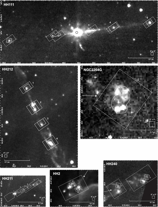
Figure 12. Outflows in our sample shown at the same spatial distance scale: spatial coverage (dashed polygons) and regions selected for extracting spectra (solid polygons) are shown on a Spitzer/IRAC channel 3 grayscale map. The position of the central driving source and the outflow direction are indicated by circles and arrows, respectively.
Download figure:
Standard image High-resolution image
Figure 13. Extracted spectra for HH 111. An additive shift of 5 × 10⁻⁸W m−2 μm−1 sr−1 was applied for illustration purposes.
Download figure:
Standard image High-resolution image
Figure 14. Extracted spectra for HH 2. An additive shift of 5 × 10⁻⁸W m−2 μm−1 sr−1 was applied for illustration purposes.
Download figure:
Standard image High-resolution image
Figure 15. Extracted spectra for HH 211. An additive shift of 5 × 10⁻⁸ W m-2 μm−1 sr−1 was applied for illustration purposes.
Download figure:
Standard image High-resolution image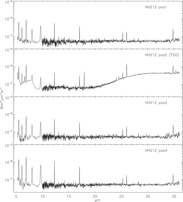
Figure 16. Extracted spectra for HH 212. An additive shift of 5 × 10⁻⁸W m−2 μm−1 sr−1 was applied for illustration purposes.
Download figure:
Standard image High-resolution image
Figure 17. Extracted spectra for HH 240. An additive shift of 5 × 10⁻⁸ W m−2 μm−1 sr−1 was applied for illustration purposes.
Download figure:
Standard image High-resolution image
Figure 18. Extracted spectra for NGC 2264 G. An additive shift of 5 × 10⁻⁸ W m−2 μm−1 sr−1 was applied for illustration purposes.
Download figure:
Standard image High-resolution image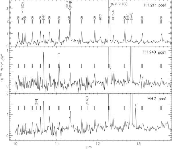
Figure 19. Spitzer/IRS SH 10–14 μm background-subtracted spectra of outflow positions with high-J OH detections (see tick marks). Strong lines are clipped for illustration purposes. The spectra were extracted from the areas indicated in Figure 12.
Download figure:
Standard image High-resolution image
Table 2. Observed, Dereddened Line Fluxes of Outflow Positions with High-J OH Detections
| ID | Flux (10−17 W m−2) | ||
|---|---|---|---|
| HH 211 – pos1 | HH 240 – pos1 | HH 2 – pos1 | |
| OH 14.6 μm (four lines) | 0.30 | 0.09 | 0.11 |
| OH 16.9 μm (four lines) | 0.42 | 0.19 | 0.28 |
| OH 20.0 μm (four lines) | 0.79 | (0.24) | 0.31 |
| H2O 30.9 μm (two lines) | 0.81 | (0.11) | (0.13) |
| OH 33.9 μm (four lines) | 1.80 | (0.31) | 0.36 |
| H2 (0−0) S(7) 5.5 μm | 72.00 | 14.00 | 20.00 |
| H2 (1−1) S(7) 5.8 μm | 4.00 | 0.36 | 0.67 |
| H2 (0−0) S(6) 6.1 μm | 31.00 | 7.10 | 17.00 |
| H2 (0−0) S(5) 6.9 μm | 86.00 | 20.00 | 29.00 |
| H2 (0−0) S(4) 8.0 μm | 39.00 | 11.00 | 20.00 |
| H2 (0−0) S(3) 9.7 μm | 77.00 | 18.00 | 15.00 |
| H2 (0−0) S(2) 12.3 μm | 18.00 | 8.20 | 5.80 |
| H2 (0−0) S(1) 17.0 μm | 6.60 | 2.20 | 1.50 |
| H2 (0−0) S(0) 28.2 μm | 0.93 | 0.45 | ... |
| [Fe ii] 5.3 μm | 3.10 | 8.10 | 4.80 |
| [Ni ii] 6.6 μm | 1.80 | 0.94 | 1.30 |
| [S iv] 10.5 μm | ... | ... | 0.14 |
| [Ni ii] 10.7 μm | 0.24 | 0.22 | 0.40 |
| [Ni ii] 12.7 μm | ... | 0.11 | 0.12 |
| [Ne ii] 12.8 μm | 0.21 | 2.10 | 14.00 |
| [Ne iii] 15.6 μm | ... | 0.11 | 1.40 |
| [Fe ii] 17.9 μm | 1.50 | 3.80 | 4.20 |
| [Ni ii] 18.2 μm | ... | ... | 0.06 |
| [S iii] 18.7 μm | ... | ... | 0.61 |
| [Fe ii]/[Fe iii] 22.9 μm | ... | 0.13 | 0.62 |
| [Fe ii] 24.5 μm | 0.34 | 0.55 | 1.10 |
| [S i] 25.2 μm | 7.40 | 0.72 | 0.72 |
| [O iv] 25.9 μm | ... | ... | 0.23 |
| [Fe ii] 26.0 μm | 4.60 | 4.30 | 4.60 |
| [S iii] 33.5 μm | ... | ... | 0.24 |
| [Si ii] 34.8 μm | 6.10 | 4.70 | 3.60 |
| [Fe ii] 35.4 μm | 1.10 | 0.76 | 0.84 |
Notes. The extraction aperture is 1.5 × 10⁻⁹ sr and upper limits are quoted in parentheses. The assumed AV-values for HH 211, HH 240, and HH 2 are 10.0, 2.5, and 0.7 mag, respectively.
Download table as: ASCIITypeset image
HH 111 at 414 pc in the L1617 cloud; highly collimated EHV outflow; near-IR spectra available (Caratti o Garatti et al. 2006); we target a total of seven knots including several high-velocity molecular bullets.
HH 2 at 414 pc in the L1617 cloud; prototypical optical bipolar outflow; bright, very young dynamical age of ∼500 years; ample near-IR and optical complementary data; consists of several 2''–5'' knots interpreted as multiple bow-shocks, winds, and fragmenting shells (Hester et al. 1998), which can be spatially resolved with Spitzer.
HH 211 at 260 pc in the IC 348 cluster; EHV outflow; near-IR spectra available (Caratti o Garatti et al. 2006; O'Connell et al. 2005); our previous spectrum detected high-J OH (Tappe et al. 2008); in this study, we extend our limited coverage to include the whole outflow.
HH 212 at 414 pc in the L1630 cloud; EHV outflow; bipolar, multiple knots and prominent terminal bow shocks; near-IR spectra available (Smith et al. 2007b); several knots and one terminal shock are MIPS 24 μm bright spots.
HH 240 at 414 pc in the L1634 globule; bipolar, multiple knots and prominent bow shocks; near-IR spectra available (O'Connell et al. 2004); position 1 is a MIPS 24 μm/[Fe ii] 1.64 μm bright spot.
NGC 2264G at 913 pc in the NGC 2264 cluster; EHV outflow; near-IR spectra available (Caratti o Garatti et al. 2006); shows [Fe ii] 1.64 μm emission associated with the CO emission peak.
Footnotes
- 4
SMART was developed by the IRS Team at Cornell University and is available through the Spitzer Science Center at Caltech.
- 5