


ABSTRACT
We investigate the effects and the implications of incorporating new collision and radiative rates in modeling the excitation of diatomic carbon molecule. The present results suggest that diffuse and translucent interstellar clouds may present a structure in which regions with different densities and kinetic temperatures overlap along the line of sight, such as core-halo clouds, the nested structure of the molecular gas, and clumpiness. Such conclusion reflects the response of the C2 rotational ladder to the interplay of thermal and radiative conditions, with low and high rotational levels tracing different regions of the parameter space. To relieve constraints to the formation and excitation of C2 molecules, we propose a scenario in which the chemistry in diffuse clouds is supplemented by chemistry in many transient and tiny perturbations.
Export citation and abstract BibTeX RIS
1. INTRODUCTION
C2, the simplest multicarbon molecule, was discovered in the interstellar medium almost 40 years ago in the near-infrared spectrum of Cyg OB2 No. 12 (Souza & Lutz 1977). Since then, diatomic carbon molecules have been extensively observed in a variety of lines of sight (e.g., Kaźmierczak et al. 2010; Wehres et al. 2010).
C2 abundance and excitation provide information on the physical conditions of interstellar clouds. The excitation of interstellar C2 in diffuse interstellar clouds was discussed by Chaffee et al. (1980), van Dishoeck & Black (1982), and van Dishoeck & de Zeeuw (1984) soon after the first detection, and subsequently by Le Bourlot et al. (1987), who updated the set of exploited molecular constants. More recently, Gredel et al. (2001) and Cecchi-Pestellini & Dalgarno (2002) investigated the diagnostic role of the distribution of C2 rotational populations in unveiling the nature of the molecular material along the line of sight toward Cyg OB2 No. 12.
van Dishoeck & Black (1982) pointed out the importance of radiative pumping and fluorescence cascade in the determination of steady-state populations of the rotational levels of the ground state. Since C2 is a symmetric molecule with no permanent dipole moment, its rotational ladder, in sharp contrast to those of heteronuclear molecules like CN or CO, may be highly populated not only by collisions, but also by radiative processes yielding excitation temperatures that are greater than the actual kinetic temperature. Providing the important molecular parameters, i.e., oscillator strengths of the involved transitions, collision cross-sections, and estimates of gas kinetic temperature, density, and radiation field intensity, theoretical rotational populations can be obtained. In turn, synthetic excitation diagrams may be used to infer kinetic temperature and density from observational data. However, care must be taken when deriving the gas physical conditions. Indeed, at the temperatures characteristic of interstellar clouds, an increase in density reduces significantly the populations of high rotational levels as the collisions drive them toward thermal equilibrium. Then, if most of the column density of C2 in the low-lying rotational levels along the line of sight resides in the diffuse gas, the high-density component may be present but undetectable (Cecchi-Pestellini & Dalgarno 2002).
The reliability of excitation diagrams as diagnostic tools of cloud properties depend critically on the correct treatment of radiative and collision rates in the balance equations. At the time of the discovery of the diatomic molecular carbon in space, there were essentially no data on C2 impact cross-sections with atomic and molecular hydrogen and helium. Collisional processes were thus estimated. In particular Chaffee et al. (1980), and subsequently van Dishoeck & Black (1982), assumed that collision rates scale in proportion with a constant cross-section, and to the statistical weights of the involved levels. Despite that later studies on the C2–H2 collision system (e.g., Phillips 1994) have made clear the very approximate nature of the original Chaffee et al. (1980) formulation of collision rates (see the next section), a number of authors (e.g., Kaźmierczak et al. 2010; Iglesias-Groth 2011) still exploit the Chaffee et al. (1980) collision scheme. Moreover, the impact of the presence of He atoms as collision partners has never been considered.
Radiative rates rely on the accurate estimate of the relevant oscillator strengths. In particular, a large number of ab initio calculations were performed for the A1Πu − X1Σ+g (Phillips) system of C2, with the derivations of radiative parameters, transition dipole moment, band oscillator strengths, and radiative lifetimes (see Kuznetsova & Stefanov 1997). With increasing computational power and instrumental sensitivity, the values of such quantities have been significantly improved in the last decade. Results obtained exploiting the original formulation of van Dishoeck & Black (1982) have been adjusted for the differences in the adopted values of the Phillips transition oscillator strengths (e.g., Kaźmierczak et al. 2010) by rescaling the density of colliders according to the prescription of van Dishoeck & de Zeeuw (1984). We recompute the radiative excitation matrix (van Dishoeck & Black 1982) exploiting recent data for the relevant molecular parameters (Section 3).
In this work, we investigate the effects and the implications of incorporating new data for both collision and radiative rates, in modeling the excitation of carbon molecule. We discuss the results through rotational excitation diagrams constructed for a sample of lines of sight where C2 absorption lines, originating from high rotational levels, have been accurately observed. In Section 5 we put forward a simple chemical model to reconcile column density observational inference and derived excitation temperatures.
2. C2 COLLISION RATES
In the van Dishoeck & Black (1982) model, which assumes constant density, the distribution of the C2 rotational levels is determined by the ratio ncσ0/I, where nc is the density of colliders, σ0 the cross-section for J = 2 → 0 quenching, and I the intensity of the incident interstellar radiation field.
De-excitation rates were assumed to depend on the square root of the temperature of the thermal bath Tk

where μ is the reduced mass of the system in amu. Based on geometrical considerations, van Dishoeck & Black (1982) estimated the value of 2 Å2 for σ0. Then, according to the Chaffee et al. (1980) prescription, downward rates result
The model by van Dishoeck & Black (1982) was subsequently updated by Le Bourlot et al. (1987) incorporating new data for the intercombination system and new collision rates, published later by Lavendy et al. (1991). The collision rate coefficients used by Le Bourlot et al. (1987) differ by factors of 2–3 with respect to the values derived by van Dishoeck & Black (1982). Le Bourlot et al. (1987) also differentiate between atomic and molecular hydrogen collisions setting impact rates with atomic hydrogen with ΔJ = 2 to one-tenth that of H2, and discarded otherwise. Later on, Phillips (1994) computed close-coupled (CC) cross-sections for rotational transitions in C2 on collision with ortho- and para-H2 for several temperatures. The derived rate coefficients were higher than the van Dishoeck & Black (1982) estimates. Moreover, the new computed rates were such that C4, 2 > C2, 0 and C6, 4 > C2, 0, in contrast to the result of the simple approximation put forward by Chaffee et al. (1980). This behavior is more pronounced with increasing temperatures. As noted by Phillips (1994), such differences arise from the use of a scaling law by Chaffee et al. (1980), that is a double (unfortunately wrong) approximation of the accurate "energy-corrected sudden with exponential power" scaling law (see DePristo et al. 1979 for details) for downward transitions in diatomic molecules
where ![$\Omega _{J,J^{\prime }} = 1/\lbrace 6+[\hbar ^{-1}\Delta \epsilon _{J,J^{\prime }}l_c\sqrt{\pi \mu /32k_BT_k}]^2\rbrace$](https://content.cld.iop.org/journals/0004-637X/749/1/48/revision1/apj421175ieqn1.gif) . Here
. Here  is the energy difference between the rotational states J and J' in cm−1, μ is the reduced mass of the system, kB is the Boltzmann constant, and lc is a scaling length (lc = 6 Å; DePristo et al. 1979).
Recently, Najar et al. (2009) presented new calculations of the rotational excitation and de-excitation of C2 (X1Σ+g) with H2, using a new ab initio potential energy surface of the van der Waals system C2–para-H2, in which H2 is in its lowest rotational level. The rates, calculated up to J = 20 in the temperature range 20–300 K, and for transitions with ΔJ = 2 and ΔJ = 4, have been compared by the authors to those derived of Lavendy et al. (1991) and Phillips (1994), with the result that remarkable differences have been evidenced, with some rates being larger and some being smaller. When Tk ≳ 100 K, the rates computed by Najar et al. (2009) are in good agreement with the results of Lavendy et al. (1991), obtained using the infinite order sudden approximation. However, at the low temperatures characteristic of interstellar clouds, only the CC method is applicable since the corresponding rate coefficients are very sensitive to the accuracy of the potential energy surface. At such temperatures Najar et al. (2009) rates show trends similar to Phillips (1994) rates, i.e., C4, 2 > C2, 0, although C6, 4 < C2, 0 at Tk ≲ 50 K. Moreover, transitions from J > 10 have collision rates comparable to, or even greater than, C2, 0. A comparison between Najar et al. (2009) and van Dishoeck & Black (1982) de-excitation rates for ΔJ = 2 transitions is shown in Figure 1 for Tk = 20, 100, and 300 K.
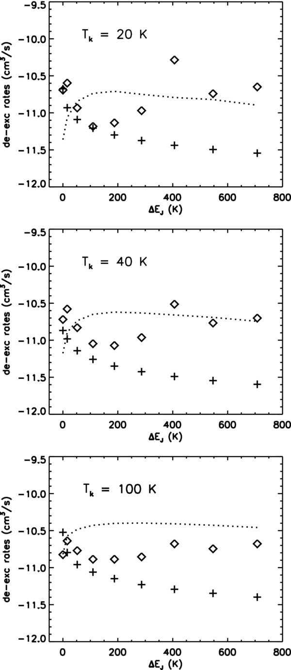
Figure 1. Collision de-excitation rates for J → J − 2 transitions in the X1Σ+g ground state as functions of the energy of the lower rotational level. +: Equations (1) and (2) with σ0 = 2 Å2 (Chaffee et al. 1980; van Dishoeck & Black 1982);  : Najar et al. (2009). Dotted lines represent de-excitation rates by He collisions (Najar et al. 2008).
Download figure:
Standard image High-resolution imageDespite the relatively large abundance of He in the cold neutral medium, the effects of He collisions with C2 has never been included in the rate equations. This is due to the approximation of collision rates that have been assumed to scale with the number density nc of an average collider. The rotational inelastic scattering of the C2 molecule in collisions with He has been theoretically studied by Robbe et al. (1992), and recently by Najar et al. (2008) for rotational transitions up to J = 20. Najar et al. (2009) compared the impact rates of C2 with H2 and those with helium. They found that such rates may differ strongly both in magnitude and shape, in a way that cannot be accounted for only by reduced mass ratio (see Figure 1). Najar et al. (2009) concluded that the different shapes of the potentials between the interacting species provide major effects. Such conclusion invalidates the assumption of an average collider.
Finally and unfortunately, no similar accurate calculations or laboratory data currently exist for C2–ortho-H2 and C2–H non reactive collisions. C2–H collisions are likely to be less relevant than C2–ortho-H2 collisions, since C2 formation should proceed more efficiently in regions in which hydrogen is mainly in molecular form. Results in the literature for different species (e.g., SO2, Cernicharo et al. 2011; methanol, Rabli & Flower 2010; SiS, Lique & Koss 2008; HCN, Dumouchel et al. 2011) show that important differences exist between the collisions with the two species of H2, involving not only intensity but also the variation with temperature. Such differences are certainly present also for collision involving C2, as implied by the differences in the corresponding potential energy surfaces (F. Najar 2011, private communication).
3. RADIATIVE RATES
We consider transitions among three electronic states of C2 arising from the excitations of valence electrons, A1Πu, D1Σ+u, and a3Πu, and its ground state X1Σ+g (see Jiang & Wilson 2011 for an accurate study of ground and excited electronic states in C2). Fluorescence processes in C2 are strongly dependent on the intercombination transitions occurring between the triplet state a3Πu and the singlet ground state (e.g., Le Bourlot & Roueff 1986). Since C2 is homonuclear, pure vibrational and rotational transitions are forbidden. Such states can be radiatively de-populated only through electronic excitations, or via  decay transitions. In other words, intercombination transitions cool down the rotational and vibrational ladders of the C2 radical.
High-accuracy data are obtained by the solution to the electronic Schröedinger equation, a complex problem that requires substantial computational effort in the case of molecules with more than two electrons. The quality of results is controlled by comparing both the radiative lifetimes and the oscillatory forces of lines and bands with the experimental values. Unfortunately, as shown by Kuznetsova & Stefanov (1997), such a comparison is subjected to a relevant number of systematic errors in the experimental values. In particular, ab initio calculations (e.g., Chabalowsky et al. 1983; van Dishoeck 1983; O'Neil et al. 1987; Langhoff et al. 1990) for the v' = 0 → v'' = 0 band of the Phillips system provide results in accord with each other, but differing substantially from the experimental data (e.g., Cooper & Nicholls 1975; Davis et al. 1984). In this work we exploit new theoretical data for the Phillips and Mulliken systems derived by Kokkin et al. (2007) and Schmidt & Bacskay (2007) using multireference configuration interaction techniques. Kokkin et al. (2007) compare the resulting radiative lifetimes of vibrational levels of the state A1Πu with the results of previous calculations and with experimental values. Computed values show a reasonable agreement with the more recent experiments (Erman & Iwamae 1995), although they appear to be larger than experimental results by a little more than the error ranges in the latter. The steep increase of the radiative lifetime with decreasing vibrational number is, however, reproduced by the calculations, while the derived lifetime of the ground vibrational state is the only prediction within the error range for the latest experimental value (Bielefeld & Meuser 1986). Subsequently, using the same technique Schmidt & Bacskay (2007) computed transition moments, oscillator strengths, and lifetimes for the Mulliken system, and recalculated these quantities for the Phillips system (and other electronic transitions) at a higher level of theory. The authors reported band oscillator strengths,  , for all transitions involving vibrational numbers in the range 0 ⩽ v ⩽ 5 for the Phillips and Mulliken systems. Finally, Franck–Condon factors for the intercombination vibrational transitions in the electronic a3Πu − X1Σ+g system are taken in Rousselot et al. (2000), who derived such quantities using a code based on the Rydberg–Klein–Rees method. The whole set of data has been exploited to construct line transition probabilities,
  , and from those the probabilities that a cascade from A1Πu and D1Σ+u, lead to X1Σ+g(0, J) (see van Dishoeck & Black 1982 and Le Bourlot et al. 1987). We briefly report the relevant relations that we used in our calculations in the Appendix (see, e.g., Thorne et al. 1999 for details).
Derived radiative excitation matrix coefficients for the Phillips and Mulliken systems are reported in Tables 1 and 2, respectively, for two different radiation fields, i.e., Mathis et al. (1982) and van Dishoeck & Black (1982). The corresponding pumping rates are virtually independent by the initial rotational level (see Table 3). The code has been tested against the original results of van Dishoeck & Black (1982) for the Phillips system. We incorporate the data inputs reported in van Dishoeck & Black (1982) and van Dishoeck (1983), with the exceptions of the energy of the involved levels, that are constructed exploiting new available data (see Rousselot et al. 2000 and references therein). We find discrepancies less than 5% for coefficients of the radiative excitation matrix of the order of 10−3 or larger. For lower values, fluctuations around the original results may be significantly larger, due to the differences in the derived transition frequencies.
Table 1. Radiative Excitation Matrix for the Phillips Systema
| Jf | ||||||||||
|---|---|---|---|---|---|---|---|---|---|---|
| Ji | 0 | 2 | 4 | 6 | 8 | 10 | 12 | 14 | 16 | 18 |
| 0 | 5.90(−1)b,c | 3.84(−1) | 2.38(−2) | 8.19(−6) | ... | ... | ... | ... | ... | ... |
| 5.93(−1)d | 3.82(−1) | 2.28(−2) | 6.35(−6) | ... | ... | ... | ... | ... | ... | |
| 2 | 8.63(−2) | 6.93(−1) | 2.09(−1) | 9.49(−3) | 3.16(−6) | ... | ... | ... | ... | ... |
| 8.57(−2) | 6.96(−1) | 2.07(−1) | 9.08(−3) | 2.44(−6) | ... | ... | ... | ... | ... | |
| 4 | 3.59(−3) | 1.13(−1) | 6.93(−1) | 1.79(−1) | 8.10(−3) | 2.83(−6) | ... | ... | ... | ... |
| 3.45(−3) | 1.13(−1) | 6.96(−1) | 1.78(−1) | 7.74(−3) | 2.19(−6) | ... | ... | ... | ... | |
| 6 | 9.18(−7) | 3.94(−3) | 1.15(−1) | 7.00(−1) | 1.71(−1) | 8.04(−3) | 2.99(−6) | ... | ... | ... |
| 7.14(−7) | 3.80(−3) | 1.15(−1) | 7.02(−1) | 1.70(−1) | 7.67(−3) | 2.31(−6) | ... | ... | ... | |
| 8 | ... | 6.65(−7) | 2.87(−3) | 1.17(−1) | 7.01(−1) | 1.69(−1) | 8.25(−3) | 3.25(−6) | ... | ... |
| ... | 5.18(−7) | 2.77(−3) | 1.18(−1) | 7.03(−1) | 1.67(−1) | 7.86(−3) | 2.50(−6) | ... | ... | |
| 10 | ... | ... | 3.79(−7) | 2.37(−3) | 1.20(−1) | 6.99(−1) | 1.69(−1) | 8.47(−3) | 3.47(−6) | ... |
| ... | ... | 2.95(−7) | 2.28(−3) | 1.20(−1) | 7.02(−1) | 1.66(−1) | 8.06(−3) | 2.68(−6) | ... | |
| 12 | ... | ... | ... | 2.93(−7) | 2.30(−3) | 1.23(−1) | 6.97(−1) | 1.69(−1) | 8.63(−3) | 3.64(−6) |
| ... | ... | ... | 2.28(−7) | 2.22(−3) | 1.23(−1) | 6.99(−1) | 1.66(−1) | 8.20(−3) | 2.80(−6) | |
| 14 | ... | ... | ... | ... | 2.97(−7) | 2.47(−3) | 1.25(−1) | 6.94(−1) | 1.67(−1) | 8.72(−3) |
| ... | ... | ... | ... | 2.31(−7) | 2.39(−3) | 1.26(−1) | 6.97(−1) | 1.65(−1) | 8.27(−3) | |
| 16 | ... | ... | ... | ... | ... | 3.45(−7) | 2.74(−3) | 1.28(−1) | 6.92(−1) | 1.76(−1) |
| ... | ... | ... | ... | ... | 2.69(−7) | 2.65(−3) | 1.28(−1) | 6.95(−1) | 1.73(−1) | |
| 18 | ... | ... | ... | ... | ... | ... | 4.16(−7) | 3.04(−3) | 1.34(−1) | 8.61(−1) |
| ... | ... | ... | ... | ... | ... | 3.24(−7) | 2.95(−3) | 1.34(−1) | 8.61(−1) | |
Notes.
aData for the transition A1Πu → X1Σ+g are taken in Schmidt & Bacskay (2007), while for the intercombination transition  in Rousselot et al. (2000).
b5.90(− 1) = 5.90 × 10⁻¹.
cRadiation field intensity derived by Mathis et al. (1982).
dRadiation field intensity derived by van Dishoeck & Black (1982).
in Rousselot et al. (2000).
b5.90(− 1) = 5.90 × 10⁻¹.
cRadiation field intensity derived by Mathis et al. (1982).
dRadiation field intensity derived by van Dishoeck & Black (1982).
Download table as: ASCIITypeset image
Table 2. Radiative Excitation Matrix for the Mulliken Systema
| Jf | ||||||||||
|---|---|---|---|---|---|---|---|---|---|---|
| Ji | 0 | 2 | 4 | 6 | 8 | 10 | 12 | 14 | 16 | 18 |
| 0 | 3.33(−1)b,c | 6.66(−1) | 7.50(−4) | 1.02(−9) | ... | ... | ... | ... | ... | ... |
| 3.33(−1)d | 6.66(−1) | 7.31(−4) | ... | ... | ... | ... | ... | ... | ... | |
| 2 | 1.33(−1) | 5.24(−1) | 3.43(−1) | 2.99(−4) | ... | ... | ... | ... | ... | ... |
| 1.33(−1) | 5.24(−1) | 3.42(−1) | 2.91(−4) | ... | ... | ... | ... | ... | ... | |
| 4 | 1.13(−4) | 1.91(−1) | 5.06(−1) | 3.03(−1) | 2.56(−4) | ... | ... | ... | ... | ... |
| 1.10(−4) | 1.91(−1) | 5.06(−1) | 3.02(−1) | 2.49(−4) | ... | ... | ... | ... | ... | |
| 6 | ... | 1.24(−4) | 2.10(−1) | 5.03(−1) | 2.87(−1) | 2.54(−4) | ... | ... | ... | ... |
| ... | 1.21(−4) | 2.10(−1) | 5.03(−1) | 2.86(−1) | 2.47(−4) | ... | ... | ... | ... | |
| 8 | ... | ... | 9.04(−5) | 2.20(−1) | 5.02(−1) | 2.78(−1) | 2.61(−4) | ... | ... | ... |
| ... | ... | 8.83(−5) | 2.20(−1) | 5.02(−1) | 2.78(−1) | 2.54(−4) | ... | ... | ... | |
| 10 | ... | ... | ... | 7.47(−5) | 2.26(−1) | 5.01(−1) | 2.73(−1) | 2.68(−4) | ... | ... |
| ... | ... | ... | 7.29(−5) | 2.26(−1) | 5.01(−1) | 2.72(−1) | 2.61(−4) | ... | ... | |
| 12 | ... | ... | ... | ... | 7.27(−5) | 2.30(−1) | 5.01(−1) | 2.69(−1) | 2.73(−4) | ... |
| ... | ... | ... | ... | 7.11(−5) | 2.31(−1) | 5.01(−1) | 2.68(−1) | 2.66(−4) | ... | |
| 14 | ... | ... | ... | ... | ... | 7.83(−5) | 2.33(−1) | 5.00(−1) | 2.66(−1) | 2.76(−4) |
| ... | ... | ... | ... | ... | 7.65(−5) | 2.34(−1) | 5.00(−1) | 2.66(−1) | 2.68(−4) | |
| 16 | ... | ... | ... | ... | ... | ... | 8.72(−5) | 2.36(−1) | 5.00(−1) | 2.64(−1) |
| ... | ... | ... | ... | ... | ... | 8.52(−5) | 2.36(−1) | 5.00(−1) | 2.64(−1) | |
| 18 | ... | ... | ... | ... | ... | ... | ... | 9.72(−5) | 2.37(−1) | 7.62(−1) |
| ... | ... | ... | ... | ... | ... | ... | 9.50(−5) | 2.38(−1) | 7.62(−1) | |
Notes.
aData for the transition D1Σ+u → X1Σg+ are taken in Schmidt & Bacskay (2007), while for the intercombination transition  in Rousselot et al. (2000).
b3.33(− 1) = 3.33 × 10⁻¹.
cRadiation field intensity derived by Mathis et al. (1982).
dRadiation field intensity derived by van Dishoeck & Black (1982).
in Rousselot et al. (2000).
b3.33(− 1) = 3.33 × 10⁻¹.
cRadiation field intensity derived by Mathis et al. (1982).
dRadiation field intensity derived by van Dishoeck & Black (1982).
Download table as: ASCIITypeset image
Table 3. Total Rates of Absorption (s−1) out of Levelsa X1Σ+g(0, J) to A1Πu and D1Σ+u
| State | Mathis et al. (1982) | van Dishoeck & Black (1982) |
|---|---|---|
| A1Πu | 2.9 × 10⁻⁹ | 3.1 × 10⁻⁹b |
| D1Σ+u | 2.4 × 10⁻¹⁰ | 4.2 × 10⁻¹⁰ |
Notes. aRates are virtually independent of J. bThe original value of the pumping rate to A1Πu derived by van Dishoeck & Black (1982) is 5.7 × 10⁻⁹ s−1, scaled by a factor 1.3 (theoretical) or 1.8 (experimental) adopting new, at that time, oscillator strengths for the Phillips system.
Download table as: ASCIITypeset image
4. RESULTS
In this section, we discuss the effects on the C2 rotational level distribution, exploiting the new collision rates computed by Najar et al. (2008, 2009), and the coefficients of the excitation matrix and pumping rates reported in Tables 1–3. We consider only transitions within the vibrational ground state X1Σ+g of C2, since collisions between higher vibrational levels are not expected to significantly affect the populations of the ground state. We solve the balance equations by means of the cascade efficiency formalism (Black & Dalgarno 1976) in the form given by Le Bourlot et al. (1987). We include cascade from A1Πu and D1Σ+u excited electronic states. Following van Dishoeck & Black (1982), we present our results in terms of relative rotational diagrams -ln[5 × NJ/(2J + 1) × N2] plotted versus ΔEJ = Δ J, 0/kB, where ΔEJ is the energy in K of the Jth rotational state with respect to J = 0, and NJ its column density. In Figure 2, we compare the results obtained through combinations of old and new data. The gas is fully molecular with a helium concentration Y = 0.1. The interstellar radiation field is taken in van Dishoeck & Black (1982), with an enhancing factor χ = 1. We consider the following cases: (a) original data from van Dishoeck & Black (1982); (b) radiative rates from Tables 1–3, and collision rates by van Dishoeck & Black (1982); (c) radiative rates from Tables 1–3, and collision rates computed by Najar et al. (2008, 2009); (d) radiative rates computed by van Dishoeck & Black (1982) and collision rates taken in Najar et al. (2008, 2009). We also modify case (c) setting Y = 0 (no helium), but increasing the gas number density in order to get the same number density of collision partners as in cases (c) and (e). Finally, case (f) has the same settings as case (c) but with a different choice for the interstellar radiation field, i.e., the one derived by Mathis et al. (1982). It is evident that the new impact cross-sections are very effective in de-exciting high rotational levels, the effect being of course more pronounced with increasing density, and tend to minimize differences provided by different radiative rates. Intensity and shape of the two adopted radiation fields do not provide appreciable differences in the population of the lowest rotational levels, although the effects can be more relevant for J ⩾ 10. Depending on the kinetic temperature, C2 may therefore thermalize easily even at relatively low hydrogen number densities. Helium collisions as well appear to be very efficient in rotational de-excitation (see also Figure 1). We thus expect that the use of updated collision rates will provide discrepancies with previous excitation analysis of observational data.

Figure 2. Synthetic excitation diagrams for C2 relative rotational populations as functions of the excitation energy, derived for two combinations of gas number density and kinetic temperature. +: case (a) (see the text); ⋆: case (b); ▵: case (c);  : case (d); □: case (e); ×: case (f). Thin solid lines describe Boltzmann distributions at the gas kinetic temperatures.
Download figure:
Standard image High-resolution imageIn obtaining the results show in Figure 2, we assume that ortho- and para-H2 collisions have identical rates. Although the Phillips (1994) calculations seem to suggest that this is actually the case, Najar et al. (2009) have clearly shown that the interaction potential surface computed by Phillips (1994) is inaccurate. We therefore look at the robustness of our calculations against variations in the collision rates of C2 with ortho-H2 and atomic hydrogen. We consider five different collision rate schemes:
- 1.
- 2.
- 3.the Chaffee et al. (1980) approximation for C2 collisions with H, Najar et al. (2009) for H2 collisions, and Najar et al. (2008) for helium collisions; in this representation the collider number density is given by nc = (x1 + x2 + Y) × nH, where x1 and x2 are the fractional abundances of atomic and molecular hydrogen (x1 + 2 × x2 = 1), and nH is total number density of hydrogen nuclei in the gas;
- 4.same as in (3), but with the use of Equation (3) for C2–H collisions;
- 5.
In exploiting model (v) we may also relax the strong assumptions made for C2 collisions with ortho-H2, scaling such rates by factors of 1/3 and 3 from those for para-H2. In the following, the adopted radiative rates are the ones reported in Tables 1–3.
In order to explore the impact of new radiative and collision rates on data analysis, we select six lines of sight containing diffuse and translucent clouds, in which reliable observations of high C2 rotational levels have been performed. Among them HD147889 and HD169454 are two translucent lines of sight (EB − V = 1.07 and 0.93, respectively; AV ∼ 3 mag) for which absorptions from (1, 0), (2, 0), and (3, 0) bands have been observed (Kaźmierczak et al. 2010), while HD27778 and HD24534 are more diffuse lines of sight (EB − V = 0.37 and 0.59, respectively) observed by Sonnentrucker et al. (2007). In addition, we present rotational diagrams derived from observations of the remarkable lines of sight toward ζ Oph (Lambert et al. 1995) and Cygnus OB2 No. 12 (Gredel et al. 2001). Not surprisingly, we failed to fit the observed rotational density columns assuming the physical conditions inferred by Kaźmierczak et al. (2010), Sonnentrucker et al. (2007), Lambert et al. (1995), and Gredel et al. (2001), unless, of course, assuming the collision model (1). More interestingly, we also failed to fit these six lines of sight using a simple homogeneous cloud model representation, i.e., single values of gas density and kinetic temperature for each line of sight. Apparently, two different physical configurations are needed: one for low J levels, and a different one for higher J. Hence, we model the observations assuming a dense component populating preferentially low J levels, mixed with a more tenuous warmer medium, whose physical conditions control the population of higher excited rotational levels. Such a scenario, initially suggested by van Dishoeck et al. (1991) for translucent clouds and by Lambert et al. (1995) for ζ Oph, has been developed by Cecchi-Pestellini & Dalgarno (2002), who considered a nested structure. We consider column densities as a superposition of the contribution from two regimes NJ = fD × N(D)J + (1 − fD) × N(d)J, where fD is the linear filling factor of the dense gas along the line of sight, and N(D)J and N(d)J are the column densities of the dense and diffuse gas, respectively. In Figure 3 we show results obtained exploiting model (v) modified assuming ortho-H2 rates scaled by a factor of 1/3 from those for para-H2, Y = 0.1, χ = 1, and x1 = 0.3 and 0.1 in the diffuse and dense phases, respectively. For comparison, we report in Table 4 results previously published by other authors for the same lines of sight.

Figure 3. Relative C2 rotational populations as functions of excitation energy (and rotational quantum number) for six lines of sight. The details of different physical models used for the fit (D: dense component, d: diffuse component; fD: percent of dense component contribution) are reported in each plot and in Table 4.
Download figure:
Standard image High-resolution imageTable 4. Physical Conditions Inferred from Observations
| Source | This Worka | |||||||||
|---|---|---|---|---|---|---|---|---|---|---|
| ncb /cm−3 | nH/cm−3 | Tk/K | ncc /cm−3 | nH/cm−3 | Tk/K | fD | ||||
| Dd | d | D | d | D | d | |||||
| HD147889 | 200 | 39 | 195 | 37.5 | 300 | 50 | 40 | 100 | 0.6 | |
| HD169454 | 326 | 19 | 325 | 37.5 | 500 | 50 | 20 | 100 | 0.7 | |
| HD27778 | 200 | 280 | 50 | 650 | 75 | 1000 | 100 | 40 | 100 | 0.3 |
| HD24534 | 200 | 325 | 45 | 390 | 37.5 | 600 | 50 | 40 | 100 | 0.5 |
| ζ Ophe | 85–225 | 125–350 | 30 | 195 | 37.5 | 300 | 50 | 40 | 100 | 0.4 |
| Cyg OB2 No. 12 | 300 | 35 | 460 | 65 | 390 | 75 | 40 | 100 | 0.35 | |
Notes. aModel (v) modified setting ortho-H2 rates equal to one-third of para-H2 rates, with Y = 0.1, χ = 1, and x1 = 0.3 and 0.1 in the diffuse and dense phases, respectively. bData in Columns 2–4 have been derived by Kaźmierczak et al. (2010) for HD147889 and HD169454, Sonnentrucker et al. (2007) for HD27778 and HD24534, Lambert et al. (1995) for ζ Oph, and Gredel et al. (2001) for Cyg OB2 No. 12. cnc = (x1 + x2 + Y) × nH. dD: dense phase, d: diffuse phase. eLambert et al. (1995) suggested the possibility that absorption from the low and high J levels originates in material with kinetic temperature Tk = 60 K but with different gas densities, nc = 175–350 and nc = 125–225 cm−3.
Download table as: ASCIITypeset image
From Table 4 we notice that kinetic temperatures of dense gas are in good agreement with results of previous rotational analyses, while in the diffuse gas kinetic temperatures are systematically larger, i.e., Tk ∼ 100 K, and consistent with T10 excitation temperatures of molecular hydrogen in the diffuse interstellar medium (e.g., Shull et al. 2000). The derived gas number densities in the denser regions are close to or larger than those derived using homogeneous models. However, number densities reported in the literature are critically dependent on the adopted values of the oscillator strengths of the involved transitions (see, e.g., Kaźmierczak et al. 2010). Indeed, C2 column densities of the lowest rotational levels yield the best estimates of kinetic temperature, while column densities of higher J levels provide tighter constraints to gas density.
5. DISCUSSION
In the previous section we show that homogeneous models fail to provide an accurate description of the C2 excitation, and, consequently, of the physical conditions of diffuse interstellar gas. Our results suggest that diffuse and translucent clouds may present a structure in which regions with different densities and kinetic temperatures overlap along the line of sight, such as core-halo clouds or nested structure of the molecular gas, and clumpiness. This is consistent with observations of ionic, atomic, and molecular species in diffuse (e.g., ζ Oph, Liszt et al. 2009) and translucent sight lines (e.g., Rachford et al. 2002; Snow et al. 2010), and more generally with the evidence for pervasive subparsec-scale structure in the diffuse interstellar medium (e.g., Boissé et al. 2009; Smoker et al. 2011). Such conclusion relies on the response of the C2 rotational ladder to the interplay of thermal and radiative conditions, with low and high J levels tracing different regions in the parameter space (see Figure 4). Absorption from high J levels requires more rarefied regions and kinetic temperatures in agreement with temperature estimates inferred from H2 measurements. The excitation temperatures of lower rotational states are coupled to the kinetic temperature of denser regions. The values of filling factors of denser regions increase in translucent clouds.

Figure 4. Relative C2 rotational populations as functions of excitation energy (and rotational quantum number) for the six lines of sight shown in Figure 3. Gas physical conditions are displayed in Figure 3 and Table 4.  : dense phase; ▵: diffuse phase. Column densities NJ are normalized with respect to NT2 = fD × N(D)2 + (1 − fD) × N(d)2.
Download figure:
Standard image High-resolution imageThere are both theoretical and observational indications that C2 formation in the diffuse gas occurs in clumps that are colder and denser than the average gas (e.g., Cecchi-Pestellini & Dalgarno 2000; Le Petit et al. 2004; Sheffer et al. 2008). Such conclusion may be in contrast with gas densities inferred by excitation analysis of C2. The use of the new collisional rates computed by Najar et al. (2008, 2009) exacerbates the dichotomy between C2 excitation and formation. In particular, the relevant timescales for thermal excitation and chemical formation differ by orders of magnitude: H2 formation in diffuse clouds occurs in about 1–3 × 10⁷ years (Liszt 2007), while collisional de-excitation timescales are of order of (1–10) × 103/(nH/cm−3) years (see Figure 1 and Section 2). The timescale for chemical evolution decreases with increasing density, but the same is true for thermal de-excitation. Thus, it is evident that it cannot help to wait for C2 formation without incurring in collisional de-activation of upper rotational states of the molecule. A possible way to remove such impasse is to postulate the existence of high density microstructure on a size scale comparable with that of the solar system (e.g., Falle & Hartquist 2002; Hartquist et al. 2003; Bell et al. 2005), that is thus overpressured and transient. An observationally suggested manifestation of such regions is the variations in atomic and molecular absorption lines on timescales of a decade or less, along many lines of sight in the diffuse interstellar medium (e.g., Rollinde et al. 2003). High density can evidently compensate for the short timescales and low extinction, so that a significant chemistry can develop even in this apparently unfavorable region of parameter space. On the other side, since such regions are expected to merge back in the embedding rarefied gas with a timescale of decades (Bell et al. 2005), there might be a phase in which fractional molecular complexity coexists with low density.
We construct a time-dependent chemical model based on the UMIST Database for Astrochemistry (UDFA; Woodall et al. 2007). We adopt a chemical network constructed from 36 species consisting of the elements H, He, C, and O, with concentrations relative to hydrogen equal to 105, 100, and 200 ppm. The cosmic-ray ionization rate has the standard UDFA value, as well as the radiation field (χ = 1). Details on computational techniques are found in Casu et al. (2001). We select from the UDFA all the reactions that couple the species. We terminate the hydrocarbon chemistry at C2H+2. The purpose of the model is to explore the chemistry that may arise in conditions apparently appropriate for the transient microstructure, i.e., rapid transition from low to high density and back, low temperature, and low extinction. As initial chemical abundances we take the equilibrium values appropriate to nH = 50 cm−3, and Tk = 100 K. The model then evolves into a dense state at nH = 2 × 104 cm−3. The value of the peak density has been assumed to be the one derived by Le Petit et al. (2004). Differences in the peak density scale the chemical evolutionary time, and change slightly the resulting fractional concentrations. We consider regions with size ΔL ∼ 10–100 AU. Such regions will form and disperse on times ∼ΔL/vd, where the velocity vd characterizes the cause of microstructure (e.g., waves traveling at the magnetosonic sound speed). Since vd is the order of 1 km s−1, the lifetime of a condensation is ∼50–500 years.
We report in Figure 5 the evolution of the fractional abundance of C2,  after an integration time of 300 years. Depending on the kinetic temperature of the condensation, the C2 fractional abundance is in the range
  . Chemical evolution follows strictly the increase in the gas density, while the gas within the microstructure falls back to the original composition on a timescale, ∼3000 years (see Figure 5), that is longer than the dispersion time of the region. In such a way, high fractional abundances are coeval with low density gas for a significant amount of time. The fast increase of concentrations in chemical species is driven by the relevant fraction of hydrogen in molecular form in the initial composition of the gas (x2 ≳ 0.4 when AV ≳ 0.05 mag; e.g., Draine & Bertoldi 1996). The abundance of C2 is controlled by the kinetic temperature in the contracting phase, being larger in colder regions. This is due to the slowing-down in the hydrocarbon formation with temperature. C2 fractional abundances are almost independent by the temperature once a steady state is reached (see the thin lines in Figure 5). We note that such condensations are not conducive to CH+ formation. Indeed, artificially opening the endothermic channel C+ + H2 → CH+ + H, we bust remarkably C2 concentration speeding up hydrocarbon build-up. In such a way, it is possible to decrease the peak density of the perturbation. However, even removing endothermicity, C2 forming perturbations cannot provide enough CH+, since this species is efficiently removed by hydrogen collisions. A similar conclusion is reached implicitly in the work of Le Petit et al. (2004), that consider the addition of shocks in order to reproduce the CH+ abundance and those of the excited rotational populations of H2.

Figure 5. Fractional abundance of C2 into the microstructure (see the text). The kinetic temperature of the contracting phase is 10 K (solid line), 50 K (dotted line), and 100 K (dashed line). Thin lines represent chemical relaxation to steady state at the corresponding kinetic temperatures.
Download figure:
Standard image High-resolution image
We briefly compare our model with observations. The aggregate column densities of high rotational levels is given by
where fM is the microstructure filling factor. In Equation (4) we assume that low density gas along the line of sight contributes mainly to populate high rotational levels (see Figure 4). Setting J⋆ = 10–18,  cm−2 for the line of sight toward HD147889 (Kaźmierczak et al. 2010), fd = 0.4 (Figure 3), and a mean C2 fractional concentration 4 × 10⁻⁸, we derive fM ∼ 0.2. Results for the lines of sight shown in Figures 3 and 4 are reported in Table 5. Such filling factors may be larger if the kinetic temperature of the contracting phase of the microstructure is higher than 10 K, or lower if the peak density in the perturbation is larger than 2 × 104 cm−3.
Table 5. Microstructure Filling Factors
| Source | E(B − V) | J⋆min |  |
fd | fM |
|---|---|---|---|---|---|
| HD147889a | 1.07 | 10 | 2.3(13)e | 0.4 | 0.2 |
| HD169454a | 0.93 | 8 | 1.0(13) | 0.3 | 0.15 |
| HD27778b | 0.37 | 6 | 1.4(13) | 0.7 | 0.24 |
| HD24534b | 0.59 | 8 | 0.9(13) | 0.5 | 0.1 |
| ζ Ophc | 0.32 | 8 | 0.6(13) | 0.6 | 0.1 |
| Cyg OB2 No. 12d | 3.31 | 6 | 7.0(13) | 0.65 | 0.14 |
Notes.  taken from (a) Kaźmierczak et al. (2010); (b) Sonnentrucker et al. (2007); (c) Lambert et al. (1995); and (d) Gredel et al. (2001). (e) 2.3(13) = 2.3 × 1013 cm−2.
Download table as: ASCIITypeset image
The results of our rather crude model suggest that it exists in a region in the parameter space which is conducive to both appreciable formation of the C2 molecule and excitation of its higher rotational levels.
6. CONCLUSIONS
In this work we estimate the impact of adopting new reliable collisional rates (Najar et al. 2008, 2009) on the rotational excitation of the dicarbon molecule. We also recompute the radiative excitation matrix (van Dishoeck & Black 1982) exploiting new data for the relevant molecular parameters (Rousselot et al. 2000; Kokkin et al. 2007; Schmidt & Bacskay 2007). Our results suggest that diffuse and translucent clouds have internal gradients in temperature and abundances. The present data are, however, unable to discriminate if the total density is continuously variable, or instead fluctuates "randomly" giving rise to a structure in which regions with different densities and kinetic temperatures are comixed.
We supplement our excitation analysis with a simple model of diffuse interstellar gas in which the chemistry in diffuse clouds incorporates the chemistry in many transient and tiny perturbations. The density of the embedding cloud may have a core-halo profile as suggested by the results in Section 3. We find that including a population of perturbations relieves some of the present constraints on the chemistry and excitation of the C2 molecule, suggesting that the microstructure may be important for interstellar chemistry (see also Cecchi-Pestellini et al. 2010). For the parameters adopted here, the filling factor of such microstructure along a typical line of sight in the diffuse interstellar medium is required to be about 10–25%. These perturbations are assumed to be of unidentified origin. Thus, the results of our chemical model should be tested by a more detailed theoretical study in which the microstructure is attributed to some specific origin such as magnetohydrodynamic waves (e.g., Falle & Hartquist 2002).
We thank the referee for comments that helped the clarity of the paper.
APPENDIX: LINE TRANSITION PROBABILITIES
The energy levels involved in the transitions are computed using the standard formula

with
and

The constants used in Equations (A1)–(A3) are reported in Rousselot et al. (2000). Definitions of F(J) for the different substates of a3Πu are given by Phillips (1968). Such relations require different constants for even and odd rotational values to account for Λ-doubling.
Band transition probabilities (s−1) are computed as follows (Kuznetsova & Stefanov 1997):
where  is the matrix element of the electron-vibrational transition (n, v' → mv''),
  is the frequency of the band origin, and a0 the radius of the first Bohr orbit. Band transition probabilities are related to the band oscillator strengths by means of the relation (van Dishoeck 1983; Thorne et al. 1999)
with λ in nm, and  and 2 for the Mulliken and Phillips systems, respectively (see Chabalowsky et al. 1983). For the intercombination transition system, the band transition probabilities are computed exploiting the relation (Rousselot et al. 2000)
where the band origin is in cm−1, 2S' + 1 the spin multiplicity,  the Frank–Condon factors, and |ΣDe|2 the transition moment (in AU) summed over the
  independent components. We assume that the two moments are equal in magnitude and independent of internuclear separation. However, the exact value of |ΣDe|2 is immaterial as long as we are interested in computing cascade factors from the states A1Πu and D1Σ+u to the ground state X1Σ+g.
Singlet system line transition probabilities are computed from the band transitions and the Hönl–London factors,  , according to
For the intercombination system a3Πu → X1Σ+g the line transition probabilities read as
The Hönl–London factors,  , are taken from the tabulation of Kovács (1969), and from Whiting et al. (1973) and Gredel et al. (1989). For singlet-triplet spin-forbidden transitions the branches are QR, PQ, and OP when N = J − 1 (1Σ → 3Π0 and 3Π2 → 1Σ transitions), R, Q and P when N = J (1Σ → 3Π1 transitions), and SR, RQ and QP when N = J + 1 (1Σ → 3Π2 and 3Π0 → 1Σ transitions). For singlet transitions, the Hönl–London factors are normalized according to the sum rule
where  for D1Σ+u and A1Πu, respectively. For the spin-forbidden transitions we follow the prescription given in Whiting & Nicholls (1974), a generalization of Equation (A9),

where  is the number of independent components of the transition moment.