


ABSTRACT
The frequency distribution of flare energies provides a crucial diagnostic to calculate the overall energy residing in flares and to estimate the role of flares in coronal heating. It often takes a power law as its functional form. We have analyzed various variables, including the thermal energies Eth of 1843 flares at their peak time. They were recorded by both Geostationary Operational Environmental Satellites and Reuven Ramaty High-Energy Solar Spectroscopic Imager during the time period from 2002 to 2009 and are classified as flares greater than C 1.0. The relationship between different flare parameters is investigated. It is found that fitting the frequency distribution of Eth to a power law results in an index of −2.38. We also investigate the corrected thermal energy Ec_th, which represents the flare total thermal energy including the energy loss in the rising phase. Its corresponding power-law slope is −2.35. Compilation of the frequency distributions of the thermal energies from nanoflares, microflares, and flares in the present work and from other authors shows that power-law indices below −2.0 have covered the range from 1024 to 1032 erg. Whether this frequency distribution can provide sufficient energy to coronal heatings in active regions and the quiet Sun is discussed.
Export citation and abstract BibTeX RIS
1. INTRODUCTION
Statistical analyses show that most of the frequency distributions of parameters related to solar active events can be characterized by power-law distributions, such as the peak flux/counts of hard X-ray (HXR) emission (e.g., Datlowe et al. 1974; Lin et al. 1984; Dennis 1985; Crosby et al. 1993; Bai 1993; Lee et al. 1993; Bromund et al. 1995; Aschwanden et al. 1995, 1998; Kucera et al. 1997; Qiu et al. 2004; Su et al. 2006), the peak flux/counts of soft X-ray (SXR) emission (e.g., Hudson et al. 1969; Drake 1971; Lee et al. 1995; Feldman et al. 1997; Veronig et al. 2002; Qiu et al. 2004; Yashiro et al. 2006; Wang et al. 2006), the peak flux/counts of radio emission (e.g., Fitzenreiter et al. 1976; Aschwanden et al. 1995, 1998; Mercier & Trottet 1997; Nita et al. 2002, 2004), the peak flux of extreme-ultraviolet (EUV) emission (e.g., Aschwanden & Parnell 2002), the flux of solar energetic particles (e.g., Van Hollebeke et al. 1975; Gabriel & Feynman 1996), the duration of flare events (e.g., Crosby et al. 1993; Bromund et al. 1995; Veronig et al. 2002; Su et al. 2006), the energy content of events (e.g., Kurochka 1987; Crosby et al. 1993; Krucker & Benz 1998; Wang et al. 2006), and the size of flaring loops (e.g., Aschwanden & Parnell 2002). For more examples see also the review by Aschwanden (2011) and references therein.
Their distributions obey the power law as

where dN denotes the number of events recorded with the variable x in the interval [x, x + dx], and δ and A are constants which can be determined by data fitting.
For the cases where x is the flare energy, Hudson (1991) pointed out that if δ is less than two, flares with higher energies play a key role in the total power; otherwise, the low energy events play a key role. A number of authors have attempted to obtain the frequency distributions of flare energies within different scale ranges in order to explore the coronal heating problem. Crosby et al. (1993) made statistics on the non-thermal electron energies greater than 25 keV observed by Solar Maximum Mission/Hard X-Ray Spectrometer. Its frequency distribution had a power-law index δ of 1.5. Hannah et al. (2008) analyzed the frequency distribution of the microflare thermal energies observed by Reuven Ramaty High-Energy Solar Spectroscopic Imager (RHESSI). It is found that overall δ was around two. Shimizu (1995) statistically analyzed the microflare events manifested as active-region transient brightenings and derived a value of 1.7 for δ. In the energy domain of nanoflares, Aschwanden et al. (2000) obtained an index of 1.8 from the statistics on the thermal energies of EUV nanoflares in the quiet Sun observed by Transition Region and Coronal Explorer (TRACE), whereas for the same observations Parnell & Jupp (2000) got a value of 2.4 and a much higher number of nanoflare events. Benz & Krucker (2002) analyzed the nanoflares in the quiet Sun observed by Extreme ultraviolet Imaging Telescope/SOHO and reached a frequency distribution similar to Parnell & Jupp (2000) with δ = 2.3. A summary of the δ values from different works gives a range from 1.5 to 2.4. They are neither all larger than two nor smaller than two. These inconsistent results make the energy budget estimation for the coronal heating more obscure.
In this paper, we are going to calculate the flare thermal energy from Geostationary Operational Environmental Satellites (GOES) and RHESSI observations. The frequency distribution of such calculated thermal energies has not been done before. In Section 2, we describe how to select the statistical sample, define the statistical variables, and analyze their relationship. In Section 3, the frequency distributions of various flare parameters are calculated. The discussions and conclusions are presented in Section 4.
2. STATISTICAL SAMPLE, VARIABLES, AND THEIR RELATIONSHIP
2.1. Statistical Sampling
For the statistics, the sampling is done for the flares observed between 2002 and 2009 according to the three criteria below.
- 1.The peak flux recorded by GOES should be larger than the C1.0 flare. We have found that about 5800 flares fulfill the criterion from the GOES flare list in Solar Geophysical Data (SGD).
- 2.The selected GOES flare should be observed by RHESSI. There are more than 2000 samples out of the 5800 GOES flares that were observed by RHESSI.
- 3.The RHESSI data should have enough signal-to-noise ratio. Thus, we have selected flares with a peak flux greater than 500 counts s−1 in the 6–12 keV energy band.In the end, our flare samples amount to 1843. The following statistics are all based on this sampling.
2.2. Statistical Variables
The temporal resolution of the data listed in SGD is one minute. Furthermore, only peak flux is recorded there, without the information on background flux. Here, we aim to obtain a more precise start and peak time for each event, and to obtain both the background and peak flux. We therefore pick up the 3 s resolution data from GOES. The new start and peak times are derived when the light curves in the 1–8 Å wavelength band during the two time intervals (90 s around the original SGD start time and 60 s around the original SGD peak time) reach the minimum and maximum, respectively. The corresponding minimum is the background flux while the maximum is the peak flux (which is used to classify SXR flares).
The statistical variables derived from GOES data are listed here. In the higher energy band from 0.5 to 4 Å, we determine its peak flux FH. In the lower energy band from 1 to 8 Å, we determine the peak flux FL, the background flux FB, the flare rising time τrise defined as the peak time minus the start time, the flare decay time τdecay defined as the end time obtained from the original SGD record minus the peak time, the duration defined as the end time minus the start time, the temperature T, and the emission measure EM at the peak time derived with the background subtracted using the standard Solar SoftWare code (White et al. 2005). A total of eight statistical variables are considered for later analyses.
The image in the 6–12 keV energy band recorded by RHESSI is utilized to obtain the area of the flare thermal emission S, and then to estimate its corresponding volume. Naturally, it would be more consistent if the thermal parameters T and EM were derived from RHESSI observations, say from the energy spectra from 6 to 12 keV. However, considering the statistical emphasis of this work, the large number of samples requires the analysis be done automatically. Unfortunately, the varying state of the attenuator aboard RHESSI makes the background energy spectra so complicated that an automated background subtraction is quite difficult. One has to manually select the start and end points in a spectrum, and choose the case-to-case-dependent background mode to perform the subtraction. Furthermore, sometimes there is no reliable energy spectrum lower than 10 keV available to derive the corresponding thermal parameters due to the influence of the attenuator on board RHESSI when in the A3 state.
The CLEAN algorithm (Hurford et al. 2002) is used for detectors 3F, 4F, 5F, 6F, 8F, and 9F to make a image, and the time integral covers 8 s around the flare peak time. To calculate the flare emission area, as done by Emslie et al. (2004), the pixels with a flux larger than 50% of the peak flux are counted. The emission volume V is then estimated by V = S3/2 accordingly. Compared with the PIXON method, a CLEAN image has the advantage of much less time consumption. The visibility forward fitting method depends on assumptions concerning the source morphology of the thermal emissions. It is quite difficult to implement automatically. Therefore, in this work the CLEAN method seems to be the most proper and robust one. For more information on the RHESSI image reconstruction methods see also Dennis & Pernak (2009) and references therein. By default, the CLEAN algorithm does not include the deconvolution of the beam size. For the example shown in Figure 1, the area in the 50% contour derived from the deconvolution-included CLEAN image is about 450 arcsec2. The default CLEAN image gives an area of about 550 arcsec2, which is about 20% larger. We estimate that the thermal energy is consequently about 16% higher.
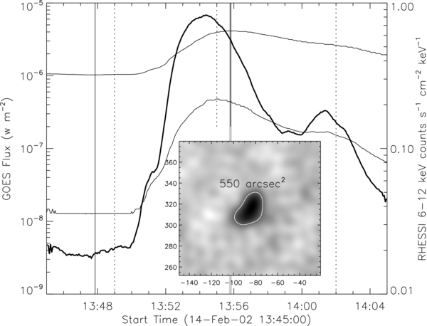
Figure 1. Example of GOES 1–8 Å, 0.5–4 Å, and RHESSI 6–12 KeV light curves. The dotted vertical lines mark the start, peak, and end times of the flare obtained from the SGD database with a one-minute temporal resolution. The refined start and peak times with a 3 s time cadence are indicated by solid vertical lines. The thickness of the second solid vertical line represents the 8 s integration time for RHESSI to make an image. On the bottom is the CLEAN image of the same flare at its peak time. The 50% contour and the corresponding area are indicated.
Download figure:
Standard image High-resolution imageCombining the derived variables from GOES and RHESSI, we obtain the electron density Ne of the hot plasma in SXR at its peak time by  . The calculation of the variable Eth in this paper follows the formula (e.g., Emslie et al. 2004; Sui et al. 2005; Li et al. 2009):

where kB is the Boltzmann constant and f is the filling factor. If f is less than one and is the same for all flares, the frequency distributions in Section 3 will have a translation to lower thermal energies but keep the power-law index unchanged. More realistically, f differs from flare to flare. Unfortunately, to our knowledge there is no good method to quantify it. Thus, in this work f is set to one.
Taking the energy loss in the rising phase into account, we have defined a corrected thermal energy  to represent the total thermal energy of a flare. If we assume that the energy loss rate in the rising phase is the same as the decay phase (Eth/τdecay), and that there is no further heating source after the SXR peak,
  has the form of

2.3. Relationships between Statistical Variables
In Figure 2, the relations of the flare peak flux FL to other flare parameters listed in Section 2.2 are presented in the log–log scale. The linear regression fittings have been done to derive the associated correlation coefficients (CCs). It is found that there are very low correlations between the flare's characteristic times and its peak flux. The CCs are not greater than 0.15. The ratio of rising and decay time shows a very poor correlation as well. For the emission area derived from RHESSI, there is almost no relationship to FL. Concerning the background flux FB, a weak correlation exists. It seems that a higher peak flux possibly comes along with a higher background flux. The temperature and density have higher CCs with FL, and Ne∝F0.5L is found.
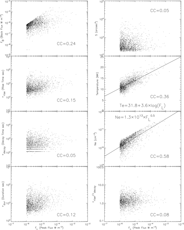
Figure 2. Scatter plots of the flare parameters as a function of the peak flux. Left column from top to bottom are for background flux, rise time, decay time, and duration; right column from top to bottom are for the emission area, temperature, density of the plasma, and τrise/τdecay. The solid lines represent the linear regression fits to the data in log–log space with the consequent regression functions indicated in the related panels. The correlation coefficients (CCs) are shown in each panel.
Download figure:
Standard image High-resolution imageFigure 3 shows the peak flux FL times flare characteristic times (e.g., τrise, τdecay, τdur) as a function of  (left column) and Eth (right column). Compared with Figure 2, the relationship presented here is quite promising. These results are consistent with the correlation analyses in Veronig et al. (2002). They found that the flare fluence, defined as flux integrated over time, had a very nice relationship to the peak flux times flare duration. Given the high CCs here, FL × τrise and FL × τdur can be utilized to estimate the thermal energy. From the linear regression analyses, we have derived the relationship of these two parameters to
  to be, respectively,
  and
and  .
.

Figure 3. Scatter plots of the flare parameters (from top to bottom: peak flux multiplied by rise time, decay time, and duration) as a function of the corrected energy (left column) and peak thermal energy (right column). The results of the linear regression fits are shown in each panel as well.
Download figure:
Standard image High-resolution image3. FREQUENCY DISTRIBUTIONS OF FLARE PARAMETERS
In this section, the frequency distributions of different flare parameters in log–log space are presented. If applicable, they are fitted by power-law distributions. In the cases below, the fittings are done with the maximum likelihood estimators (Clauset et al. 2009). The lower boundary of the fitted quantity is determined automatically by this method. The upper boundary is the maxima of the corresponding flare parameter. We find that even though there are a few noisy points at the higher end, the power-law index is not affected too much. The deviations in the power-law distributions are determined by the Kolmogorov–Smirnov, or KS, statistic (Press et al. 1992).
In Figure 4, the frequency distributions of FL, FL/τrise, FL/FB, and FH are displayed. Here, FL/τrise represents the averaged non-thermal flux according to the Neupert effect (Su et al. 2006). All the distributions can be nicely fitted by power-law functions with their corresponding indices of 2.04, 2.25, 1.90, and 1.85. A closer inspection indicates that, except for the case of FL/τrise, most of the flare samples obey the power-law distribution. We have to note that minor deviations to the power-law distributions exist in the lower range of the measurements. Compared with the index of 2.11 FL in Veronig et al. (2002), our results are quite close to theirs. In general, the frequency distribution of the non-thermal peak flux is relatively harder, with its power-law index around 1.8 (e.g., Crosby et al. 1993; Su et al. 2006). However, we find that the index associated with FL/τrise is even softer than the SXR peak flux. To explain this result, further studies are needed.

Figure 4. Frequency distributions as a function of the peak flux, peak flux/rise time, peak flux/background, and flux in the high energy channels at peak time. The straight lines indicate the data fittings by the maximum likelihood estimators.
Download figure:
Standard image High-resolution imageThe frequency distributions of T, EM, and Ne at flare peak time, and the flare emission area S are presented in Figure 5. It is shown that EM and S follow the power law and the corresponding indices are 2.02 and 2.65, whereas the plasma T and Ne do not, and the distribution of temperature has the shape of a Gaussian with a hump in the higher temperature tail. Considering the logarithm scale in the Y axis, the enhancement of flare numbers in higher temperatures is actually quite limited. The distribution is peaked at T ≈ 12 MK. About 87% of the analyzed flare samples have temperatures between 8.5 MK and 15.5 MK. The deficiency of flares in lower temperatures with respect to the Gaussian distribution is probably due to instrument sensitivity.
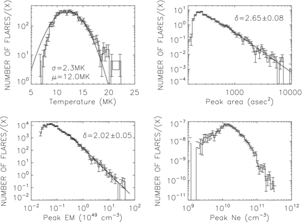
Figure 5. Frequency distributions as a function of temperature, EM, area, and density of the plasma at peak time. The distribution as a function of temperature is fitted by a Gaussian function with the μ = 12 MK and σ = 2.3 MK. The straight lines have the same meaning as in Figure 4.
Download figure:
Standard image High-resolution imageThe frequency distributions of the thermal energies Eth and  (Figure 6) are most attractive in this work. Their power-law fittings produce indices of 2.38 and 2.35, respectively. The thermal energy at flare peak time Eth covers the range from 8 × 1028 to 3 × 1031 erg. The total thermal energy
  spans from 8 × 1028 to 3 × 1032 erg. It can be seen that the index related to Eth is a little bit softer than the one associated with
  . A possible explanation could be that often a larger flare has bigger τrise/τdecay (see Figure 1), and therefore has more additional corrected energy loss.
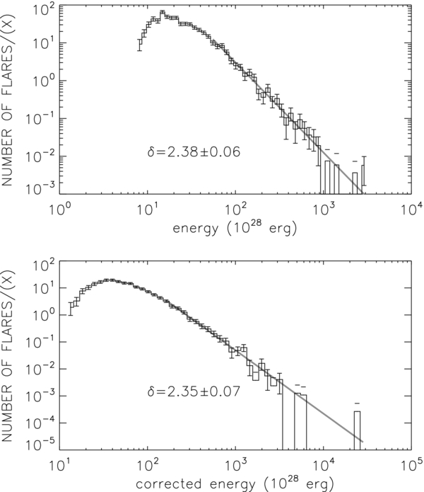
Figure 6. Frequency distributions as a function of thermal energy and corrected thermal energy. The straight lines have the same meaning as in Figure 4.
Download figure:
Standard image High-resolution imageThe energy coverage in the frequency distribution spans three magnitudes for our flare samples greater than C1.0 class. It is one magnitude narrower than the one in Veronig et al. (2002) in which all the GOES flare list events are considered. Such a selection bias has an influence on the frequency distribution of thermal energy, e.g., a higher turn-over value in Figure 6. According to Aschwanden & Charbonneau (2002), flare sampling with a narrow temperature range might affect the power-law index and produce a weaker power-law distribution than the unbiased sampling. However, our flare samples have an energy coverage broad enough to obtain a reliable power-law index. In Figure 6, the turn-over point determined by the maximum likelihood method is indeed close to the C 5.0 flare if we assume that the thermal energy is proportional to its peak flux. Even if we extend flare samples down to a B class flare, we expect that the power-law index does not change much and is still greater than two since it is mostly determined by the data points above the turn-over point.
To compile the frequency distributions of flare energies in the context of the results from other authors, we normalized the differential flare frequency in units of s−1 cm−2 erg−1 by the visible surface area of the Sun and the duration of observation (2002–2009), as done in Aschwanden et al. (2000) and Hannah et al. (2008). The result is shown in Figure 7. Concerning the normalization, we have taken into account that RHESSI did not observe all flares during the observations from 2002 to 2009. For all of the 5800 flares greater than C level recorded during this period, RHESSI only had observations available for 1843 flares. For the normalization of the frequency distribution in Figure 7, we multiplied the flare number in Figure 6 with a factor of 5800/1843. In other words, the integrated total number of flares in Figure 6 is 1843, but this number is increased to 5800 in Figure 7. By combining the statistics based on the data from different instruments, the power-law distributions have now been extended to a broader flare energy range which is from 1024 to 1032 erg. Their frequency distributions can be classified into two categories: one with a power-law index δ less than two (e.g., Crosby et al. 1993; Aschwanden et al. 2000; Shimizu 1995), and the other group with δ greater than two (e.g., Parnell & Jupp 2000; Benz & Krucker 2002; and the present work).

Figure 7. Composite flare frequency distribution in a normalized scale and in units of 10−50 flares s−1 cm−2 erg−1. The diagram includes the flares analyzed in this work (abbreviated as GL) from Hannah et al. (2008, RH), Benz & Krucker (2002, EB), Aschwanden et al. (2000, TA), Parnell & Jupp (2000, TP), Shimizu (1995, SS), and Crosby et al. (1993, SC). The slopes of −2.0 and −2.3 are extrapolated to the entire energy domain from 1024 to 1032 erg.
Download figure:
Standard image High-resolution image
4. DISCUSSIONS AND CONCLUSIONS
In this paper, we have performed statistical analyses of 1843 flares larger than the C1.0 class which were observed by GOES and RHESSI during the period between 2002 and 2009. The frequency distribution of their peak thermal energies can be fitted quite well by a power-law function having an index of −2.38. After correcting the flare heating losses, we made statistics on the total thermal energies. The corresponding frequency distribution produces an index of −2.35.
From Figure 7, we can see that our power-law index is consistent with the ones derived by Benz & Krucker (2002) and Parnell & Jupp (2000) based on the TRACE nanoflare statistics. Thus, the index around −2.3 deduced from the frequency distribution of flare thermal energies is valid within a broader energy range which is now extended from 1024 to 1032 erg. However, the empty space in the energy scale of the microflare still needed to be filled. Interestingly, the SS (Shimizu 1995) got close to our power-law fitting line and the slope at their higher energy part looks quite close to our results as well.
Aschwanden et al. (2007) estimated the requirement of heating power density according to the energy balance in the corona and found a value of ∼105 erg cm−2 s−1 for quiet-Sun regions and ∼106 erg cm−2 s−1 in active regions. On the other hand, the energy supply to coronal heating can be calculated from the frequency distribution of flare energies (e.g., Hudson 1991):
where W is the total energy power density provided by flares, and N(E) is the differential frequency distribution of flare energies derived in Section 3 which has the functional form of A E−δ.
It has been proved in Hudson (1991) that if δ > 2, then the total power density produced by flares depends on the less energetic events, that is, the integral lower limit Emin has a greater effect on W. On the contrary, in the cases where δ < 2, the value of Emax is more important to W. If flares at different energy scales can provide the energy required for the heating in quiet Sun and active regions, Emax or Emin have to reach the magnitude listed in Table 1 in which different frequency distributions are considered.
Table 1. The Magnitude of Energy Upper or Lower Limits (Emax or Emin in erg) Calculated from Equation (4) on the Condition that the Energy Budgets Estimated from Different Cases of Frequency Distributions are Capable to Fulfill the Heating Requirements for the Quiet Sun (QS) and Active Regions (AR)
| Case | QS | QS | AR | AR |
|---|---|---|---|---|
| (min) | (max) | (min) | (max) | |
| TA | ... | 1037 | ... | 1041 |
| SC | ... | 1035 | ... | 1037 |
| SS | ... | 1034 | ... | 1037 |
| TP | 1021 | ... | 1019 | ... |
| EB | 1024 | ... | 1021 | ... |
| GL | 1023 | ... | 1020 | ... |
Download table as: ASCIITypeset image
Concerning the coronal heating in the quiet Sun, it can be seen from Table 1 that in the cases of frequency distributions with δ > 2, EB and GL have Emin around 1024 and 7 × 10²³ erg, respectively. Therefore, it can be concluded that flares with energy between 1024 and 1032 erg are able to meet the requirement of corona heating in the quiet Sun.
With regard to the issue of active-region heating, we similarly derive Emax for the three frequency distributions with δ < 2. They are 1041, 1037, and 1037 erg for the cases of TA, SC, and SS, respectively. Accordingly, we calculated the corresponding probabilities of the events with energy greater than 1034 erg by  . We found that these high energy events should occur about 5, 7, or 33 times per 11 years to provide sufficient heating to active regions. However, such grand flare events have not been observed in the frequency estimated above during the past few solar cycles.
In the cases of frequency distributions with δ > 2, we find that flare energy has to be extended to about 1020 erg in order to heat active regions. The energy interval between 1024 and 1032 erg can provide only 10% of the total heating requirement for active regions. The remaining 90% of heating sources are hiding in the currently undetectable energy band from 1020 to 1024 erg. If we assume a plasma temperature of 2 MK and density of 108 cm−3, then the spatial scale of flares with energy of 1020 erg is around 100 km. We can expect an even smaller scale if the temperature and density are higher. Furthermore, the occurrence rate of such small-scale flares is estimated to be 20 arcsec−2 s−1. Up to now, there has been no detector with such a spatial and temporal resolution to observe the flares with energies below 1020 erg. It could be important in the future to test if the same power-law index around −2.3 could be extended downward to an energy of 1020 erg.
The above discussions assumed that the total energy in the range from nanoflares to regular flares is uniformly distributed in the full solar disk, which is either all covered by quiet regions or all covered by active regions. However, realistically the solar disk is often covered by the quiet Sun and active regions at the same time. The coronal heating problem in active regions and the quiet Sun is different.
The frequency distribution derived from EUV observations in the energy range between 1024 and 1028 erg is dedicated to the heating of the quiet Sun. Benz & Krucker (2002) pointed out that microevents in the quiet corona and regular flares in active regions are statistically different. Therefore, the energy distribution of the EUV microflares in the quiet Sun cannot be extrapolated to active regions. However, Aschwanden et al. (2000) found some uniform scaling laws as a function of temperature for both active regions and the quiet Sun. Hence, a power-law distribution with the same index can be valid in the range from 1024 to 1032 erg. The regular flares analyzed in this work only occurred in active regions. The power-law index of their energy distribution is consistent with the one derived from the events in the quiet Sun, i.e., the results derived from the EUV nanoflares in EB and TP. We also found a similar result derived from the microflares in the work of SS.
In reality, flares, especially those big ones, only occur and release energy in active regions. The normalization of their frequency distributions should also take the parameters of active regions. Suppose we normalize the distribution of the regular flares by the area of active regions instead of the visible surface area of the Sun, its frequency distribution would be lifted, and its power-law fitting would still be parallel to the thick line in Figure 7. In other words, in Equation (4) the coefficient A would increase, and the index δ would be the same. If we apply the same procedure to the results in SS, which was normalized by the area of the full disk in Aschwanden et al. (2000) and Hannah et al. (2008), the corresponding frequency distribution would increase by the same level as our flare distribution. Note that the SS result represents the frequency distribution of the microflares in active regions. For active-region heating, the same frequency distribution could then be extended from the regular flares to microflares. According to our energy estimate in Equation (4), if A increases, then the derived Emin would increase as well, which would be higher than the previous value of 1020 erg. As long as the power-law distribution can be extrapolated to the calculated Emin, the total integrated energy extended to nanoflare or even less energetic scales could be sufficient to heat active regions. To our knowledge, there have been no statistics on nanoflares in active regions. We hope that some clues can be achieved with the Atmospheric Imaging Assembly observations on board the Solar Dynamics Observatory.
We thank the referee for comments which greatly improved our manuscript. The authors thank the GOES and RHESSI consortia for supplying their data. Y.P. Li and W.Q. Gan were supported by NSFC grants (10833007, 11078025, and 11173063) and 973 Program (2011CB811402); L. Feng was supported by NSFC grant 11003047.