


ABSTRACT
The astrophysical reaction rates of 12C(α,γ)16O below T9 = 3, calculated from the potential model, are provided in tabular form and as analytic expressions. The uncertainties of the reaction rates are estimated by using variations of the model parameters.
Export citation and abstract BibTeX RIS
1. INTRODUCTION
The 12C(α, γ)16O reaction is considered as the key reaction for the carbon–oxygen ratio in the universe, and it influences not only the production of all elements heavier than A = 16 nuclei, but also stellar evolution from the He-burning phase to the explosive phase (Rolfs & Rodney 1988). The knowledge of 12C(α, γ)16O, however, has not been established yet, because the energy near the Gamow window corresponding to He-burning temperatures (Ec.m. = 0.3 MeV) is too low to measure the cross section in present laboratories. In the sequence of reactions in He burning, 3α → 12C(α, γ)16O(α, γ)20Ne, the reaction rates of the triple-α process is comparatively well determined experimentally through the study of the resonance at the excitation energy Ex = 7.65 MeV in 12C. The 16O nuclei cannot be consumed significantly, because there is no resonance in 20Ne at the astrophysically interesting energies. At present, the low-energy 12C(α, γ)16O cross section, from which the reaction rate is derived, is a remaining unsolved problem. Current theoretical discussions about the α-capture reactions are available at, e.g., Katsuma (2008), Mohr (2005), Ogata et al. (2009), and Dufour & Descouvemont (2008).
Recently, precise measurements of γ-ray angular distributions (Assunção et al. 2006; Makii et al. 2009; Kunz et al. 2001; Ouellet et al. 1996; Redder et al. 1987), cascade transitions (Kettner et al. 1982; Redder et al. 1987; Matei et al. 2006), and β-delayed α spectra for 16N (Buchmann & Barnes 2006; Tang et al. 2010 and references therein) have been performed to understand the low-energy 12C(α, γ)16O reaction more thoroughly. The phase shifts of α + 12C elastic scattering at low energies have been investigated to describe accurately the initial scattering channel (Plaga et al. 1987; Tischhauser et al. 2009). Through these experimental studies, the extension of the cross section to low energies has been extrapolated. Other experimental information are available in Dyer & Barnes (1974), Kremer et al. (1988), Barker & Kajino (1991), Buchmann et al. (1993, 1996), Azuma et al. (1994), Ouellet et al. (1996), Trautvetter et al. (1997), Angulo & Descouvemont (2000), Kunz et al. (2001), Tischhauser et al. (2002), Kettner et al. (1982), Barker (1987), Roters et al. (1999), Buchmann (2001), Hammer et al. (2005), Schürmann et al. (2005), Redder et al. (1987), and Matei et al. (2006). The extrapolation has also been predicted by the studies of the indirect measurements (6Li,d) and (7Li,t), e.g., Belhout et al. (2007) and Brune et al. (1999). Despite these efforts, uncertainties still remain in the astrophysical reaction rates at the important He-burning temperatures, T9 ≈ 0.1–0.2 (T9 is defined by T = T9 × 109 K).
Representative results for the reaction rate have been provided by Kunz et al. (2002, 2001), Buchmann (1996), Buchmann et al. (1996), Azuma et al. (1994), and Buchmann et al. (1993), based on the R-matrix analyses of the radiative capture data, the β-delayed α spectrum of 16N, and the phase shifts for elastic scattering. In this article, their results are referred to as KU02 (Kunz et al. 2002, 2001) and BU96 (Buchmann 1996; Buchmann et al. 1996; Azuma et al. 1994; Buchmann et al. 1993). For the extrapolated astrophysical S factors at Ec.m. = 0.3 MeV, KU02 estimate SE1 = 76 ± 20 keV b, SE2 = 85 ± 30 keV b, and Scasc = 4 ± 4 keV b for the E1, E2, and cascade transitions. BU96 predict SE1 = 79 ± 21 keV b, SE2 = 70 ± 70 keV b, and Scasc = 16 ± 16 keV b. The derived reaction rates give different temperature dependences from that in the Fowler's pioneering compilation of the reaction rates (Caughlan & Fowler 1988, hereafter CF88).
The NACRE compilation (Angulo et al. 1999) is the milestone work after CF88, providing evaluated reaction rates for the astrophysical community. For 12C(α, γ)16O, the NACRE reaction rate is based on the results from the R-matrix method of Buchmann et al. (1993) and Azuma et al. (1994) for E1 and Barker & Kajino (1991) for E2. Their extrapolated values at Ec.m. = 0.3 MeV are SE1 = 79 ± 21 keV b and SE2 = 120 ± 60 keV b. It is assumed that the contribution from the cascade transition through the excited states in 16O is negligible. The contribution from resonances up to Ec.m. = 6 MeV is added separately. The NACRE reaction rates of the 12C(α, γ)16O reaction now seem somewhat out-of-date compared with the recommended rates from the recent experimental and theoretical works.
The low-energy α+12C cross sections have been investigated with microscopic models (e.g., Dufour & Descouvemont 2008; Descouvemont & Baye 1987; Descouvemont et al. 1984). Hybrid models have also been performed in, e.g., Langanke & Koonin (1985), Funck et al. (1985), Langanke & Koonin (1983), and Koonin et al. (1974). The qualitative analyses by the models may seem successful. The effects of coupling to other channels were taken into account theoretically. But they might not have described 12C(α,γ)16O with sufficient accuracy, because of the limitations of their models. Besides, the coupling included explicitly might be redundant for the low-energy α+12C reaction because elastic scattering can be described by the single channel calculation of Katsuma (2010a).
For the evaluation of the reaction rates, the E1 contribution from the 1−1 state at Ex = 7.12 MeV, just below the α-particle threshold of 16O, is assumed to play a crucial role in the reproduction of the available data at low energies. Our recent theoretical study (Katsuma 2008) using the potential model, however, shows that the low-energy cross section is dominated by the E2 component. The additive contribution from the 1−1 state does not seem to be necessarily required. The derived S factors at Ec.m. = 0.3 MeV are SE1 = 3 keV b, SE2 = 150 keV b, and Scasc ≈ 20 keV b. Moreover, Katsuma (2008) illustrates that the derived reaction rate is concordant with published rates at the He-burning temperatures, even if the low-energy E1 cross section is not enhanced by the subthreshold 1−1 state. Our potential model is constructed so as to satisfy the semi-classical limit of α-clustering aspect deduced by the optical potential describing rainbow phenomena at high energies (Katsuma 2008). Additional information from comments and replies is available in Descouvemont et al. (2010) and Katsuma (2010b).
The α+12C elastic scattering provides the initial channel for the direct capture potential model. The result from Katsuma (2010a), using the empirical potential (Katsuma 2008), gives a successful reproduction of the elastic differential cross sections, especially the enhancement of backscattering. It also shows survival of the single-particle motion of α-particle in the excitation function below Ec.m. = 5 MeV. Katsuma (2010a) endorses the applicability of the potential model with a simple α+12C configuration.
In this article, the numerical values of the 12C(α, γ)16O reaction rate below T9 = 3 are listed in a tabular form. By performing a polynomial expansion of the reaction rates, a simple analytic expression is proposed. To estimate the theoretical uncertainties, we examine the sensitivity to the model parameters. The phase shifts of α + 12C elastic scattering are used to guide the variation of the potential parameters. The main purpose of this article is to distribute the theoretical reaction rates for assessment in astrophysical applications. The difference between our reaction rate and others (KU02; BU96; NACRE; CF88) originates from the assumed reaction mechanism in the analysis of the 12C(α, γ)16O cross section. We assume a direct capture mechanism and adopt the simple potential model. We take account of the contribution from the cascade transition through the excited states of 16O.
In the following section, we describe the procedure for estimating the reaction rates. In Section 3, the sensitivity of the 12C(α, γ)16O cross sections to the model parameters is investigated. The reaction rates are compared with KU02, BU96, NACRE, and CF88 and are given in tabular form and by an analytic expression. We examine the reaction rates deduced from the new phase-shift data of Tischhauser et al. (2009). A summary is given in Section 4.
2. THEORETICAL REACTION RATES
The reaction rates of the 12C(α, γ)16O reaction are estimated from the potential model. The model used in this article is the same as that in the previous work (Katsuma 2008). We describe here the theoretical reaction rates, the procedures for estimating uncertainties, and analytic expressions. The details of the model can be found in Katsuma (2008).
The Maxwellian averaged thermonuclear reaction rate (Rolfs & Rodney 1988; Angulo et al. 1999) is defined by
where NA, kB, μ, and T are the Avogadro number, Boltzmann constant, reduced mass, and temperature, respectively. Ec.m. is the center-of-mass energy. The σ(Ec.m.) is the capture cross section obtained from the potential model with a simple α + 12C configuration, and it is given as
where ϕf and ϕi are the wave functions for the final bound state and initial scattering channel, respectively. MEλ is the electromagnetic operator of the Eλ transition with the effective charge. The λ is the multipolarity of the transition; kγ is the wave number of γ-rays; v is the relative velocity; d0 is the factor depending on the orbital angular momentum and λ.
The effective charge in the electromagnetic operator is expressed with ![$\tilde{e}^{E\lambda }= e[Z_1(A_2/A)^\lambda + Z_2(-A_1/A)^\lambda ]$](https://content.cld.iop.org/journals/0004-637X/745/2/192/revision1/apj412062ieqn1.gif) (Barker & Kajino 1991; Descouvemont 2003), where A1(Z1) and A2(Z2) are mass number (charge) of nuclei in the initial channel and A = A1 + A2. However, the effective charge is treated as an adjustable parameter in our model (Katsuma 2008), including corrections in normalization of the transition amplitude. For example, the effective charge for the E1 transition is
(Barker & Kajino 1991; Descouvemont 2003), where A1(Z1) and A2(Z2) are mass number (charge) of nuclei in the initial channel and A = A1 + A2. However, the effective charge is treated as an adjustable parameter in our model (Katsuma 2008), including corrections in normalization of the transition amplitude. For example, the effective charge for the E1 transition is  . This may express the isospin selection rule. However,
  can be a small value due to violation of the isospin selection rule. The normalization also originates from the simplicity of the model. It may depend on the assumption of the direct capture. The final bound state may have the complicated nuclear structure, which reflects to a spectroscopic factor deviating from unity. The effective charge is basically a part of the electromagnetic operator leading to the transition from the scattering channel to the bound state. It is, however, expressed as a value depending on the final bound state
  because of the inclusion of the spectroscopic factor.
To generate the initial waves ϕi, we use the parity-dependent potential,
where ξ denotes the "+" (even) and "−" (odd) parities of the scattering channel. For the final bound state, the same functional form of the potential is used, of which the strength parameter is adjusted to reproduce the α-particle separation energy. In the case of the final bound state, ξ is used as a label of the state, assigned in order of the excitation energy. The method generating the bound state with the experimental particle separation energy is generally implemented in the direct reaction calculations (Satchler 1983) using, for example, the distorted-wave Born approximation. For the Coulomb potential, we use the uniform charge sphere with a radius RC = 3.5 fm.
In our potential model (Katsuma 2008), the given potentials generate both the initial and final wave functions. The effective charges  of the bound state are adjusted so as to minimize the difference between the experimental and theoretical cross sections (Assunção et al. 2006; Kunz et al. 2001; Kettner et al. 1982; Redder et al. 1987; Matei et al. 2006). The reaction rates are obtained from the numerical integrals of the calculated cross section, including the extrapolated values. Thus, it is a difficult task to find reasonable parameters of the potential.
The astrophysical S factor is used to compensate for the rapid variation of the cross section below the Coulomb barrier and is defined by

where η is the Sommerfeld parameter, η = Z1Z2e2/(ℏv); Z1 and Z2 are the charges of interacting nuclei.
Before describing the procedure for estimating the uncertainties, let us recall the results from Katsuma (2008).
- 1.At low energies, the S factor is dominated by the E2 transition to the 16O ground state, whereas the E1 component is not enhanced by the subthreshold 1−1 state. The E2 component originates from the 2+1 state (Ex = 6.92 MeV).
- 2.The cascade transitions through the excited states below the α-particle threshold are not very important below Ec.m. = 1 MeV.
- 3.The reaction rates above T9 = 1 cannot be determined without reference to the cascade transition of the 3−1 state (Ex = 6.13 MeV).
These imply the following.
- (A)The variation of the even-parity potential leads to the different energy dependence of the E2 cross section.
- (B)Above T9 = 1, the unknown cascade transition to the 3−1 state of 16O produces a large part of the uncertainties.
We estimate the uncertainties of the S factor and reaction rates by variation of the model parameters, i.e., the even-parity potential and the 3−1 effective charge.
To examine (A), we use the even-parity potentials (Katsuma 2008) labeled as P4a–P4g in Table 1, which are obtained from a χ2 fit to the phase-shift data (Plaga et al. 1987). The χ2ps is defined by
where δexl and δthl are the experimental and theoretical phase shifts, respectively. Δδl is the uncertainty of the data, assumed to be Δδl = 1°. The angular momentum has values of l = 0, 2, 4. Figure 1 shows the differences in the reproduction of the phase shifts. The solid curves are calculated from the best-fit parameters (P4d). The dotted and dashed curves are obtained from P4b and P4f, respectively. The phase shifts vary smoothly with the listed potential. In this article, we presume that the parameter sets of P4b–P4f are within the theoretical uncertainty. The odd-parity potential is fixed to V− = 168.1 MeV, R− = 2.76 fm, and a− = 0.567 fm.
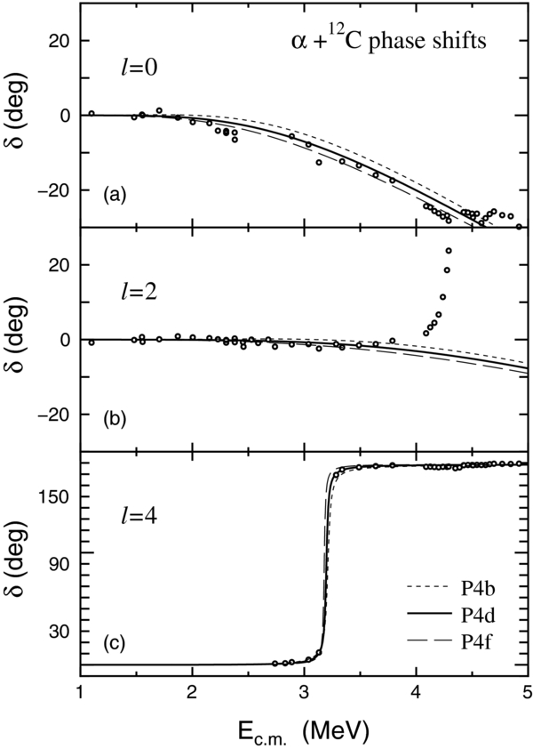
Figure 1. Phase shifts of α+12C elastic scattering for (a) l = 0, (b) l = 2, and (c) l = 4. The solid curves are the results calculated from the best-fit parameters (P4d). The dotted and dashed curves are obtained from P4b and P4f, respectively. The parameters are listed in Table 1. The experimental data are taken from Plaga et al. (1987).
Download figure:
Standard image High-resolution imageTable 1. Parameters of the Even-parity Potential
| Potentials | R+ | V+ | a+ | χ2ps/94 |
|---|---|---|---|---|
| (fm) | (MeV) | (fm) | ||
| P4a | 2.05 | 204.2 | 0.831 | 8.79 |
| P4b | 2.10 | 202.0 | 0.801 | 5.74 |
| P4c | 2.15 | 200.5 | 0.766 | 4.02 |
| P4d | 2.18 | 199.7 | 0.743 | 3.74 |
| P4e | 2.20 | 199.4 | 0.726 | 3.86 |
| P4f | 2.25 | 199.5 | 0.674 | 5.16 |
| P4g | 2.28 | 203.7 | 0.608 | 6.52 |
Download table as: ASCIITypeset image
For (B), the E2 effective charge of the 3−1 state is varied within the range of  . In Katsuma (2008), it was assumed that
  .
.
An analytic expression of the reaction rate is useful not only to implement the astrophysical applications but also to understand the contributions to the reaction rates. Several types of the analytic expression have been considered (Rolfs & Rodney 1988; Caughlan & Fowler 1988; Angulo et al. 1999). We try to express the reaction rate by using only a few parameters, as one of the forms:
where hn,  (n = 0–3), and gn (n = 1, 2) are the coefficients of the expansion, which are adjusted to make the appropriate reaction rates. Although g1 is given by g1 = 3(π2μ/(2kB))1/3(e2Z1Z2/ℏ)2/3 ≈ 32.1, it is adjusted to make a good approximation. The expression of Equation (7) is adopted in the NACRE compilation. The leading term at low temperatures in both equations appears to originate from the subthreshold state, as described in Section 3.3. The other terms do not have any specific mechanisms, but are used for the polynomial expansion, so the negative values of the coefficient do not have a special interpretation. The deviation between the analytic expression and tabular rate is defined by
where NA〈σv〉Eq and NA〈σv〉Table are the analytic expression and the tabular value, respectively. The accuracy of the expansion is characterized by the maximum value of Δ.
The theoretical reaction rates in the temperature T9 = 0.012–3.0 region are calculated with the potential model. The values of T9 are the same in the table of CF88 (Caughlan & Fowler 1988). However, the reaction rate at T9 = 0.012 is too small; the order of magnitude is approximately 10−50 cm3 mol−1 s−1. In the NACRE compilation, the reaction rates below 10−25 cm3 mol−1 s−1 are assumed to be practically negligible for all astrophysical conditions. Thus, the tabular rates for T9 = 0.04–3.0 are provided in this article. This choice of the lowest temperature is the same as that in KU02 (Kunz et al. 2002). When making an analytic expression, the reaction rates in the entire region are taken into account to reproduce the theoretical model. Above T9 = 3, the uncertainties of the reaction rates are expected to increase because of the contribution from the experimental data concerning narrow resonances. Moreover, the unknown 3−1 cascade transition leads to the uncertainties (Katsuma 2008). We truncate the reaction rates at T9 = 3 because the rates above T9 = 3 do not correspond to the range of the considered cross section data.
3. RESULTS
In this section, we indicate the sensitivity of the S factor to the variation of the model parameters and compare the theoretical rate with the published rates (KU02; BU96; NACRE; CF88). The uncertainties of the reaction rates are also discussed. After listing the numerical values of the reaction rates, we present polynomial expansions with Equations (6) and (7), and provide a recommended expression. We finally discuss the results from the new phase-shift data of Tischhauser et al. (2009).
3.1. S Factors
The astrophysical S factors of the E2 transition for the 12C(α, γ0)16O reaction are shown in Figure 2. The solid curve is the result calculated with the parameter set of P4d, which is the same curve as in Figure 5 of Katsuma (2008). The dotted and dashed curves are obtained from P4b and P4f, respectively. The E1 and E2 effective charges of the ground state, listed in Table 2, are adjusted to minimize the difference between the experimental and theoretical cross sections. The E2/E1 ratio seems reasonable from the angular distribution of γ-rays (Katsuma 2008).
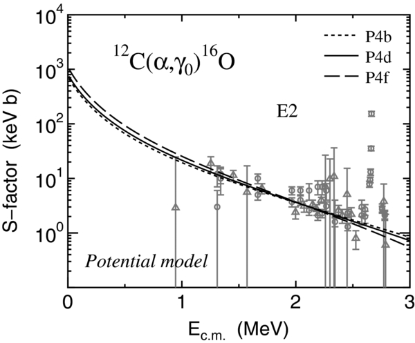
Figure 2. Astrophysical S factors of the E2 component for the 12C(α,γ0)16O reaction. The solid curve is the result calculated with the parameter set of P4d (Table 1). The dotted and dashed curves are obtained from P4b and P4f, respectively. The experimental data are taken from Assunção et al. (2006) and Kunz et al. (2001).
Download figure:
Standard image High-resolution imageTable 2. Sensitivity of the S Factors at Ec.m. = 0.3 MeV and Derived Effective Charges of the Ground State
| Potentials |  |
 |
SE1 | SE2 |
|---|---|---|---|---|
| (10−3 e) | (e) | (keV b) | (keV b) | |
| P4a | 8.33 | 1.16 | 3.0 | 121 |
| P4b | 8.80 | 1.29 | 2.9 | 133 |
| P4c | 9.46 | 1.54 | 2.9 | 140 |
| P4d | 9.96 | 1.69 | 2.9 | 150 |
| P4e | 10.38 | 1.86 | 2.9 | 156 |
| P4f | 11.97 | 2.37 | 2.9 | 191 |
| P4g | 15.20 | 3.57 | 3.0 | 257 |
Download table as: ASCIITypeset image
In Table 2, the obtained S factors are listed. The E2 S factor varies smoothly, and it is found to be SE2 = 150+41−17 keV b at Ec.m. = 0.3 MeV, if the potentials of P4b, P4c, P4d, P4e, and P4f with the optimized effective charges are adopted. In contrast, SE1 ≈ 3 keV b is estimated. Although we examined the sensitivity of the S factor by varying the odd-parity potential keeping the l = 1, 3 phase shifts, the resultant E1 S factor was hardly affected.
To examine the sensitivity of the total S factor to the variation of the parameters, the cascade transitions must be taken into account. The effective charges of the excited states are listed in Table 3, as well as those of the ground state. The  of 0+2, 2+1, and 1−1 are obtained from the fits to the cross section data (Kettner et al. 1982; Redder et al. 1987; Matei et al. 2006). The values
  , 1.4, and 2.8 e are used for the 3−1 cascade transition. At Ec.m. = 0.3 MeV, the resultant S factor of the cascade transitions is ScascE1 + E2 = 18 ± 4.5 keV b. The total S factor is, therefore, found to be StotE1 + E2 = 171+46−22 keV b.
Table 3. E1 and E2 Effective Charges of the Bound States
| Potentials |  |
 |
 |
 |
 |
 |
 |
 |
 |
 |
|---|---|---|---|---|---|---|---|---|---|---|
| (10−3 e) | (e) | (10−3 e) | (e) | (10−3 e) | (e) | (10−3 e) | (e) | (10−3 e) | (e) | |
| P4a | 8.33 | 1.16 | 0. | 1.77 | 0. | 0., 1.4, 2.8 | 4.50 | 2.03 | 0. | 1.38 |
| P4b | 8.80 | 1.29 | 0. | 1.86 | 0. | 0., 1.4, 2.8 | 5.54 | 2.07 | 0. | 1.38 |
| P4c | 9.46 | 1.54 | 0. | 1.97 | 0. | 0., 1.4, 2.8 | 4.96 | 2.37 | 0. | 1.38 |
| P4d | 9.96 | 1.69 | 0. | 2.05 | 0. | 0., 1.4, 2.8 | 5.33 | 2.48 | 0. | 1.38 |
| P4e | 10.38 | 1.86 | 0. | 2.11 | 0. | 0., 1.4, 2.8 | 6.17 | 2.49 | 0. | 1.38 |
| P4f | 11.97 | 2.37 | 0. | 2.32 | 0. | 0., 1.4, 2.8 | 9.63 | 2.21 | 0. | 1.38 |
| P4g | 15.20 | 3.57 | 0. | 2.63 | 0. | 0., 1.4, 2.8 | 14.43 | 1.27 | 0. | 1.38 |
Download table as: ASCIITypeset image
We now discuss what is known about the asymptotic normalization constants (ANC; Mukhamedzhanov & Tribble 1999; Mukhamedzhanov et al. 1995). The α-particle ANC is defined by  , where W(r) is the Whittaker function. Sα is the α-particle spectroscopic factor, given by
  in our model (Katsuma 2008). The ANCs of the bound states used in the calculation of the recommended reaction rates shown in the next subsection are C2 = 5.01 × 1028 fm−1, 2.03 × 10¹⁰ fm−1, 1.18 × 10⁴ fm−1, 2.76 × 10⁶ fm−1, and 3.00 × 10⁵ fm−1 for 1−1, 2+1, 3−1, 0+2 (Ex = 6.05 MeV), and 0+1 (ground state). The ANC and Sα seem to be consistent with previous analyses (Belhout et al. 2007; Brune et al. 1999; Sparenberg 2004).
The calculated lifetime and B(E2) of the 2+1 state allow the model to be assessed. The lifetime t = 5.98+0.72−3.33 fs and B(E2; 2+1 → 0+1) = 8.62+10.8−0.93 e2 fm4 values are obtained from the parameters of Tables 1 and 3. The density distribution of α-particle (Satchler & Love 1979) and 12C (Kamimura 1981) are used. The α-particle spectroscopic factor of 2+1 is assumed to be Sa = 1. The evaluated value is t = 6.78 ± 0.19 fs (Tilley et al. 1993).
3.2. Reaction Rates
In Figure 3, the reaction rates obtained from the potential model are compared with the published rates: (a) CF88, (b) NACRE, (c) KU02, and (d) BU96. In each panel, the theoretical reaction rates are indicated with the ratio to the respective reaction rates. The solid curves are the ratio of our recommended reaction rates. For reference, the ratio of the upper (lower) limit evaluated by NACRE, KU02, and BU86 is indicated with the dotted (dashed) curve. There is no indication of the dotted and dashed curves in Figure 3(a) because CF88 do not provide the uncertainties. Below T9 ≈ 0.4, our reaction rates are within the uncertainties of NACRE, KU02, and BU96. From Figure 3 one sees that our reaction rates resemble BU96 in the temperature dependence, rather than CF88 and NACRE. Our reaction rate has a different trend with temperature compared with CF88 and NACRE, and shows a steep slope with increasing T9. At high temperatures, the deviation from NACRE and CF88 mainly originates from the contribution of the cascade transition. The contribution from the experimental narrow resonances stemming from the compound nucleus mechanism is not analyzed in this paper.
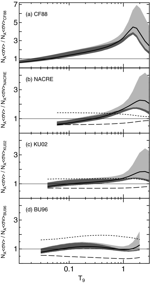
Figure 3. Comparison between the reaction rates. The present reaction rates are indicated by the ratios to the recommended rates in (a) CF88 (Caughlan & Fowler 1988), (b) NACRE (Angulo et al. 1999), (c) KU02 (Kunz et al. 2002, 2001), and (d) BU96 (Buchmann 1996; Buchmann et al. 1996; Azuma et al. 1994; Buchmann et al. 1993). The solid curves are the ratio of the recommended reaction rates, while the pale and dense shade regions show the uncertainties estimated in this article (see the text). For reference, the ratio of the upper (lower) limit evaluated by the respective articles is indicated with the dotted (dashed) curve.
Download figure:
Standard image High-resolution imageThe uncertainties of the reaction rates obtained from the variation of the parameters are illustrated by the shaded areas in Figure 3. The pale shade is the uncertainty estimated from the variation of the potential parameters and  . The dense shade is with fixed
  . We confirm from this figure that the uncertainties at low temperatures stem from the potential variation. In contrast, the large part of the uncertainties above T9 = 1 originates from the cascade transition through the 3−1 state. To put the reaction rates on a firm foundation, measurement of the 3−1 cascade cross section would be required. Conceivably, the 3−1 cascade cross section may be as important as contributions from narrow resonances in the 1 < T9 < 3 temperature region. The recommended values have been calculated by assuming that the effective charge of the 3−1 state is approximately equal to that of the 1−1 state (Katsuma 2008). The uncertainties estimated here appear to be reduced at low temperatures compared with other evaluations.
The numerical values of the present reaction rate are listed in Table 4, including the upper and lower limits. The reaction rates are given in units of cm3 mol−1 s−1. The values in each row should be multiplied by 10n, where n is listed in the sixth row.
Table 4. Theoretical 12C(α,γ)16O Reaction Rates
| T9 | Low | Recommend | High | NACREa | 10n |
|---|---|---|---|---|---|
| 0.04 | 6.14 | 6.84 | 8.96 | ⋅⋅⋅ | −31 |
| 0.05 | 4.03 | 4.50 | 5.86 | ⋅⋅⋅ | −28 |
| 0.06 | 5.59 | 6.25 | 8.11 | 10.2 | −26 |
| 0.07 | 2.84 | 3.18 | 4.11 | 4.98 | −24 |
| 0.08 | 7.20 | 8.07 | 10.4 | 12.2 | −23 |
| 0.09 | 1.10 | 1.23 | 1.58 | 1.80 | −21 |
| 0.10 | 1.15 | 1.29 | 1.64 | 1.81 | −20 |
| 0.11 | 8.83 | 9.91 | 12.6 | 13.5 | −20 |
| 0.12 | 5.37 | 6.02 | 7.66 | 7.98 | −19 |
| 0.13 | 2.69 | 3.02 | 3.83 | 3.89 | −18 |
| 0.14 | 1.15 | 1.29 | 1.63 | 1.61 | −17 |
| 0.15 | 4.27 | 4.80 | 6.05 | 5.86 | −17 |
| 0.16 | 1.42 | 1.60 | 2.01 | 1.91 | −16 |
| 0.18 | 1.19 | 1.32 | 1.67 | 1.53 | −15 |
| 0.20 | 7.30 | 8.20 | 10.2 | 9.11 | −15 |
| 0.25 | 2.76 | 3.09 | 3.81 | 3.21 | −13 |
| 0.30 | 4.32 | 4.84 | 5.93 | 4.75 | −12 |
| 0.35 | 3.84 | 4.31 | 5.24 | 4.03 | −11 |
| 0.40 | 2.31 | 2.60 | 3.14 | 2.31 | −10 |
| 0.45 | 1.06 | 1.18 | 1.42 | 1.00 | −9 |
| 0.50 | 3.86 | 4.32 | 5.16 | 3.52 | −9 |
| 0.60 | 3.27 | 3.66 | 4.33 | 2.75 | −8 |
| 0.70 | 1.79 | 2.01 | 2.37 | 1.40 | −7 |
| 0.80 | 7.25 | 8.14 | 9.61 | 5.36 | −7 |
| 0.90 | 2.36 | 2.66 | 3.16 | 1.66 | −6 |
| 1.00 | 6.56 | 7.42 | 8.87 | 4.41 | −6 |
| 1.25 | 5.15 | 5.96 | 7.57 | 3.19 | −5 |
| 1.50 | 2.60 | 3.13 | 4.40 | 1.53 | −4 |
| 1.75 | 9.79 | 12.6 | 19.8 | 5.76 | −4 |
| 2.00 | 3.04 | 4.19 | 7.15 | 1.84 | −3 |
| 2.50 | 1.92 | 2.85 | 5.26 | 1.27 | −2 |
| 3.00 | 7.71 | 11.9 | 22.0 | 5.81 | −2 |
Notes. The reaction rates are in units of cm3 mol−1 s−1. aNACRE reaction rates (Angulo et al. 1999).
Download table as: ASCIITypeset image
3.3. Analytic Expression of the Reaction Rates
We find a polynomial expansion of the tabular form of the reaction rates using Equation (6). The coefficients of the expansion are listed in Table 5. The maximum deviations, defined by Equation (8), are 6%, 8%, and 7% for the recommended, the upper limit, and the lower limit of the rates. The tabular reaction rates are satisfactorily expressed by Equation (6). The coefficients are |hn| < 1 (n = 1, 2, 3). The reaction rate is thus found to be dominated by the first term at low temperatures.
Table 5. Coefficients of the Expansion of the Theoretical Reaction Rates, Defined by Equation (6)
| Tabular Form | h0 | h1 | h2 | h3 | g1 | g2 | Max. Δa |
|---|---|---|---|---|---|---|---|
| (cm3 mol−1 s−1) | |||||||
| Recommend | 1.16 × 10⁹ | −0.371 | −0.106 | 0.264 | 32.369 | 3.17 | 6% |
| High | 1.32 × 10⁹ | −0.0686 | −0.845 | 0.711 | 32.330 | 2.80 | 8% |
| Low | 1.02 × 10⁹ | −0.422 | 0.124 | 0.0894 | 32.363 | 4.04 | 7% |
Note.a The maximum deviation is defined by Equation (8).
Download table as: ASCIITypeset image
A better expression could not be found with Equation (7) adopted in NACRE. The coefficients for the recommended reaction rates are listed in Table 6.  becomes large,
  . Taking T9 = 0.1, for example, the reaction rate is found to be dominated by the second term.
Table 6. The Same as Table 5, but the Coefficients Are Defined by Equation (7)
| Tabular Form |  |
 |
 |
 |
g1 | g2 | Max. Δ |
|---|---|---|---|---|---|---|---|
| (cm3 mol−1 s−1) | |||||||
| Recommend | 9.04 × 10⁶ | 186.3 | −189.8 | 88.6 | 32.189 | 3.45 | 16% |
Download table as: ASCIITypeset image
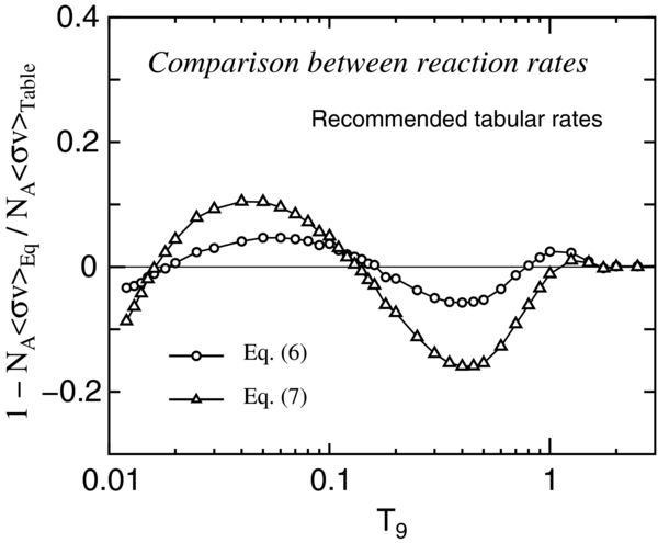
Figure 4 makes a comparison between the analytic expression and the tabular form. For the recommended reaction rates, the deviations 1 − NA〈σv〉Eq/NA〈σv〉Table are indicated with the circles (Equation (6)) and triangles (Equation (7)). Around T9 = 0.05 and 0.4, the analytic expressions deviate from the recommended tabular rates.
Figure 4. Comparison between the analytic expression and the tabular form. For the recommended reaction rates, 1 − NA〈σv〉Eq/NA〈σv〉Table are indicated with the circles (Equation (6)) and triangles (Equation (7)). The maximum deviations, defined by Equation (8), are 6% and 16% for the circles and triangles, respectively. The lines are used to guide the eye.
Download figure:
Standard image High-resolution image
Let us consider the reaction mechanism associated with Equation (6). Using Equation (14) of Angulo et al. (1999) with ωγ = 0, the contribution from the subthreshold state, NA〈σv〉SR, is expressed in units of cm3 mol−1 s−1 as follows:

where S(E0) is the S factor in MeV b units at the most effective energy E0 (Rolfs & Rodney 1988; Angulo et al. 1999) approximately given as E0 ≈ 0.922T2/39 MeV for the considered reaction (Angulo et al. 1999). Suppose the slope of the S factor is simplified with S∝1/Ec.m., then T−2/39 dependence is found in S(E0). The corresponding reaction rate implicitly depends on T−4/39. The T−29 dependence is found if S∝1/E2c.m. is assumed. It thus seems that the first term of Equation (6) is the so-called tail contribution from the subthreshold state, having a weak energy dependence.
If S(E0) = 0.17 MeV b is substituted into Equation (9), the coefficient becomes 2 × 10⁹. This appears to be in the same order of magnitude as h0 (Table 5). For the expression of Equation (7),  is small compared with 109, while
  becomes comparable (Table 6). We thus consider the analytic expression of Equation (6) to be better than that of Equation (7) for the present reaction rates because it is easier to understand the reaction rates at low temperatures. Besides, the accuracy of Equation (6) is good.
At high temperatures, the analytic expression of Equation (6) consists of the contributions from the total S factor and includes the cascade transitions. The resonant contributions of the states belonging to the α + 12C rotational band in 16O are also included. Therefore, the polynomial expansion does not have any specific interpretation.
3.4. Discussion about the New Phase Shift Data
We assemble the new data for l = 0, 2, 4 from Tischhauser et al. (2009) to determine the even-parity potential. In accordance with Katsuma (2008), l = 2 data for Ec.m. > 4 MeV are not included. δexl = 0 is excluded in the χ2ps fit. l = 6 data are not included because they are almost zero in the energy range. Thus, the number of data points is 331 (l = 0), 190 (l = 2), and 323 (l = 4). The s-wave phase shift of Tischhauser et al. (2009) seems to deviate slightly from that of Plaga et al. (1987).
The even-parity potential is calculated so as to minimize the χ2ps value defined by Equation (5). With the fixed R+, the sensitivity of the potential is examined around the P4 (Katsuma 2008) minimum of the χ2ps surface. We additionally impose the constraint on the potential to reproduce the α-particle separation energy of the 2+1 state. The resultant parameters are listed in Table 7. The potential giving the χ2ps minimum is labeled as P4d'. The radius parameter of P4d' is slightly larger than R+ = 2.18 fm of P4d (Table 1). P4d' is identical to P4e.
Table 7. Parameters of the Even-parity Potential Obtained from the Data of Tischhauser et al. (2009)
| R+ | V+ | a+ | χ2ps/844 |
|---|---|---|---|
| (fm) | (MeV) | (fm) | |
| 2.05 | 203.8 | 0.8337 | 24.5 |
| 2.10 | 201.6 | 0.8042 | 14.9 |
| 2.15 | 200.0 | 0.7694 | 8.0 |
| 2.18 | 199.5 | 0.7445 | 5.3 |
| 2.20 | 199.4 | 0.7256 | 4.3a |
| 2.22 | 199.75 | 0.7029 | 4.7 |
| 2.25 | 201.9 | 0.6548 | 8.6 |
| 2.26 | 204.3 | 0.6250 | 12.1 |
| 2.27 | 206.0 | 0.6004 | 65.9 |
Note.a P4d'.
Download table as: ASCIITypeset image
The small change mentioned above does not lead to a large difference of the reaction rates in the present method.
4. SUMMARY
The theoretical 12C(α, γ)16O reaction rates below T9 = 3 have been considered with the potential model, and they have been provided in tabular form and by an analytic expression. The uncertainties of the reaction rates and cross sections have been estimated from the variation of the model parameters. The even-parity potential and 3−1 effective charge are varied. As a guide to the variation of the potential parameters, the sensitivity of the phase shifts for α + 12C elastic scattering was examined.
At Ec.m. = 0.3 MeV, the S factor is estimated to be SE2 = 150+41−17 keV b for the E2 component. The uncertainties of the E1 and cascade transitions are not so important as that of SE2. The E1 S factor is SE1 ≈ 3 keV b. The S factor of the cascade transition is ScascE1 + E2 = 18 ± 4.5 keV b. Therefore, the total S factor is StotE1 + E2 = 171+46−22 keV b.
The reaction rates are listed in Table 4, as well as the upper and lower limits, and they are compared with KU02, BU96, NACRE, and CF88. Although the assumed reaction mechanism is different, the reaction rate seems to be concordant with the published rates at low temperatures. The temperature dependence of our reaction rates is similar to that of BU96.
The recommended reaction rates for T9 ⩽ 3 are expressed as
in units of cm3 mol−1 s−1. The maximum deviation from the tabular reaction rate is 6%. The first term appears to represent the tail contribution from the subthreshold 2+1 state and dominates the reaction rate at low temperatures. For the present rates, the expression beginning with T−4/39 (Equation (6)) is superior to that with T−29 (Equation (7)). The upper and lower limits, NA〈σv〉H and NA〈σv〉L, are given by
The maximum deviations are 8% and 7%, respectively.
The author thanks Professors Y. Sakuragi, A. Kawauchi, and Y. Ohnita for their comments and encouragement, and thanks Professor I. J. Thompson for a careful reading of the manuscript. He also thanks Professors P. Descouvemont, M. Dufour, J.-M. Sparenberg, and A.E. Champagne for calling his attention to the present problem. He is grateful to Professors M. Arnould, A. Jorissen, K. Takahashi, and H. Utsunomiya for their hospitality and encouragement during his stay at Université Libre de Bruxelles (ULB). He thanks anonymous referee for comments. This work has been done in part by the Interuniversity Attraction Pole IAP 5/07 of the Belgian Federal Science Policy (Konan University—ULB convention), and was partially supported by the JSPS institutional program for young researcher overseas visits, "Promoting International Young Researchers in Mathematics and Mathematical Sciences led by Osaka City University Advanced Mathematical Institute."