


ABSTRACT
We report the discovery of HAT-P-25b, a transiting extrasolar planet orbiting the V = 13.19 G5 dwarf star GSC 1788-01237, with a period P = 3.652836 ± 0.000019 days, transit epoch Tc = 2455176.85173 ± 0.00047 (BJD—barycentric Julian dates throughout the paper are calculated from Coordinated Universal Time, UTC), and transit duration 0.1174 ± 0.0017 days. The host star has a mass of 1.01 ± 0.03 M☉, radius of 0.96+0.05− 0.04 R☉, effective temperature 5500 ± 80 K, and metallicity [Fe/H] = +0.31 ± 0.08. The planetary companion has a mass of 0.567 ± 0.022 MJ and radius of 1.190+0.081− 0.056 RJ yielding a mean density of 0.42 ± 0.07 g cm−3.
1. INTRODUCTION
As more transiting extrasolar planets (TEPs) are discovered, statistics become significant enough to begin looking at bulk properties of exoplanet populations. By investigating relationships between stellar, planetary, and orbital characteristics (see, e.g., Hartman et al. 2011; Burrows et al. 2007; Enoch et al. 2011), we can probe the underlying astrophysics that dictates the properties we observe. In this paper, we present the discovery of HAT-P-25b, the 25th TEP found by the Hungarian-made Automated Telescope Network (HATNet; Bakos et al. 2004) survey, orbiting the star also known as GSC 1788-01237.
With V = 13.19, HAT-P-25 was the faintest transiting planet host star discovered by a wide-field, ground-based transit survey at the time of its discovery—the recently announced hot-Jupiter TrES-5b (Mandushev et al. 2011) orbits a V = 13.72 star. Traditionally wide-field surveys using small-aperture telescopes, such as HAT, WASP, XO, and TrES, have focused on stars with V < 13 mag while fainter stars have been the domain of space-based surveys and narrow-field ground-based surveys such as OGLE (e.g., OGLE-TR-56b, V = 16.6; Konacki et al. 2003), CoRoT (e.g., CoRoT-1b, V = 13.3; Barge et al. 2008), and Kepler (e.g., Kepler-5b, V = 13.4; Koch et al. 2010). As these latter surveys have shown, spectroscopically confirming planets around faint stars poses several challenges which are not present for brighter hosts (e.g., Pont et al. 2008).
HATNet has been one of the main contributors to the discovery of TEPs. In operation since 2003, it has now covered approximately 14% of the sky, searching for TEPs around bright stars (8 ≲ I ≲ 14.0). HATNet operates six wide-field instruments: four at the Fred Lawrence Whipple Observatory (FLWO) in Arizona and two on the roof of the hangar housing the Smithsonian Astrophysical Observatory's Submillimeter Array, in Hawaii.
The layout of the paper is as follows. In Section 2, we report the detection of the photometric signal and the follow-up spectroscopic and photometric observations of HAT-P-25. In Section 3, we describe the analysis of the data, beginning with the determination of the stellar parameters, continuing with a discussion of the methods used to rule out non-planetary, false positive scenarios which could mimic the photometric and spectroscopic observations, and finishing with a description of our global modeling of the photometry and radial velocities. Our findings are discussed in Section 4.
2. OBSERVATIONS
2.1. Photometric Detection
The transits of HAT-P-25b were detected with the HAT-10 telescope in Arizona and the HAT-9 telescope in Hawaii. The region around GSC 1788-01237, a field internally labeled as 259, was observed on a nightly basis between 2008 September 15 and 2009 March 16, whenever weather conditions permitted. We gathered 6786 exposures of 5 minutes at a 5.5 minute cadence. Each image contained approximately 36,000 stars down to Sloan r ∼ 14.5. For the brightest stars in the field, we achieved a per-image photometric precision of 4 mmag.
The calibration of the HATNet frames was carried out using standard photometric procedures. The calibrated images were then subjected to star detection and astrometry, as described in Pál & Bakos (2006). Aperture photometry was performed on each image at the stellar centroids derived from the Two Micron All Sky Survey (2MASS; Skrutskie et al. 2006) catalog and the individual astrometric solutions. The resulting light curves were decorrelated (cleaned of trends) using the external parameter decorrelation (EPD; see Bakos et al. 2010) technique in "constant" mode and the trend filtering algorithm (TFA; see Kovács et al. 2005). The light curves were searched for periodic box-shaped signals using the box least-squares (BLS; see Kovács et al. 2002) method. We detected a significant signal in the light curve of GSC 1788-01237—also known as 2MASS 03134450+2511506; , δ = +25°11'50 7; J2000; V = 13.19 (The Amateur Sky Survey, TASS; Droege et al. 2006)—with an apparent depth of ∼15.1 mmag, and a period of P = 3.6528 days (see Figure 1). The drop in brightness had a first-to-last-contact duration, relative to the total period, of q = 0.0321 ± 0.0005, corresponding to a total duration of Pq = 2.817 ± 0.041 hr (see Figure 1).


Figure 1. Unbinned (top) and binned (bottom) light curves of HAT-P-25 including all 6786 instrumental Sloan r band 5.5 minute cadence measurements obtained with the HAT-9 and HAT-10 telescopes of HATNet (see the text for details), and folded with the period P = 3.6528362 days resulting from the global fit described in Section 3. The solid line shows the "P1P3" transit model fit to the light curve (Section 3.3).
Download figure:
Standard image High-resolution image2.2. Reconnaissance Spectroscopy
As is routine in the HATNet project, all candidates are subjected to careful scrutiny before investing valuable time on large telescopes. We used two facilities to carry out the reconnaissance spectroscopy: the Tillinghast Reflector Echelle Spectrograph (TRES; Fűrész 2008) on the 1.5 m Tillinghast Reflector at FLWO and the FIbre-fed Echelle Spectrograph (FIES; Frandsen & Lindberg 1999) on the 2.5 m Nordic Optical Telescope (NOT; Djupvik & Andersen 2010) at La Palma, Spain. Both of these instruments provide high-resolution spectra which, with even modest signal-to-noise ratios (S/Ns), are suitable for deriving radial velocities (RVs) with moderate precision (≲ 0.1 km s−1) for slowly rotating stars. The reconnaissance observations are summarized in Table 1. Below we provide a brief description of each instrument, the data reduction, and the analysis.
Table 1. Reconnaissance Spectroscopy of HAT-P-25
| Instrument | BJD | RVa | Teff⋆b | log g⋆ | vsin i |
|---|---|---|---|---|---|
| (2,454,000+) | ( km s−1) | (K) | ( km s−1) | ||
| TRES | 1113.87949 | −12.417 ± 0.036 | 5250 ± 125 | 4.0 ± 0.25 | 6.0 ± 1.0 |
| FIES | 1115.67533 | −12.608 ± 0.036 | 5250 ± 125 | 4.0 ± 0.25 | 4.0 ± 1.0 |
Notes. aThe velocities reported here are the result of a multi-order cross-correlation against the IAU standard HD182488 and have been shifted to the absolute velocity scale of Nidever et al. (2002). The errors are calculated from the rms scatter of individual orders in the multi-order analysis. This error estimate does not include possible systematic errors due to, e.g., template mismatch or uncorrected instrumental drifts. bThe stellar parameters Teff⋆, log g⋆, and vsin i are the result of correlation of a single order against a grid of synthetic spectra with assumed [Fe/H] = 0. Errors quoted are half of the grid spacing, but do not take into account systematic errors introduced if HAT-P-25 has non-solar metallicity.
Download table as: ASCIITypeset image
Our first spectrum was taken with the medium fiber on TRES, which has a resolving power of λ/Δλ ≈ 44, 000 and a wavelength coverage of ∼3900–8900 Å. The second spectrum was taken with the medium fiber on FIES, which has resolving power of λ/Δλ ≈ 46, 000 and a wavelength coverage of ∼3600–7400 Å. The spectra were extracted and analyzed according to the procedures outlined by Buchhave et al. (2010). Having monitored the IAU radial velocity standard HD182488 over the span of about 400 days with both TRES and FIES, we can compare the velocity zero points and stability of each instrument to determine if any correction must be applied before combining the data sets. We calculate the mean TRES velocity to be −20.821 ± 0.060 km s−1 (rms error) when correlations are performed in a single echelle order against a synthetic spectrum. For FIES, this number is −20.890 ± 0.046 km s−1. From this, we conclude that velocities from TRES and FIES are on the same velocity scale (to within the errors), and for the purposes of detecting velocity variation due to a stellar companion (tens of km s−1), no offset need be applied.
Based on the reconnaissance spectroscopy, we find that the system has rms velocity residuals consistent with no velocity variation within the measurement precision, and the observations show no evidence of a composite spectrum. From this, we conclude that HAT-P-25 has no stellar companion. Furthermore, the surface gravity found by each instrument is consistent with a dwarf star, which reduces the likelihood that the HATNet detection is caused by a background blend.
While we found the reconnaissance velocities to be consistent with each other to within the measurement precision, these velocities were calculated by making use of only one order of each spectrum, a small wavelength range (∼80 Å) surrounding the Mg i b triplet. By cross-correlating two spectra against each other order by order and summing the correlation functions, we can utilize the information in a larger wavelength range, effectively increasing the S/N and reducing the measurement errors. In doing so, we may be able to detect a statistically significant velocity variation indicative of a planetary companion or at least place an upper limit on the mass of any such companion. For the multi-order cross-correlation, we used observed templates—spectra of the IAU standard HD182488 taken on the same night as each HAT-P-25 spectrum—to perform the analysis. This allowed us to shift each relative velocity to the IAU scale and look for orbital motion. We used the wavelength range ∼4400–6650 Å, and the resulting velocities are shown in Table 1. The revised velocities imply Mp = 0.74 ± 0.19 MJ, assuming a mass of 1 M☉ for HAT-P-25, an estimate from the classification of the reconnaissance spectra. We note that the error does not take into account systematic uncertainties due to template mismatch, which could affect the relative velocities; or the stability of the instruments, which could affect the combination of the relative velocities onto the absolute scale.
2.3. High-resolution, High-S/N Spectroscopy
We obtained high-resolution, high-S/N spectra of HAT-P-25 using the HIRES instrument (Vogt et al. 1994) on the Keck I telescope located on Mauna Kea, Hawaii, between 2009 December and 2010 February. The width of the spectrometer slit was 086, resulting in a resolving power of λ/Δλ ≈ 55, 000, with a wavelength coverage of ∼3800–8000 Å.
Eight exposures were taken through an iodine gas absorption cell, which was used to superimpose a dense forest of I2 lines on the stellar spectrum and establish an accurate wavelength fiducial (see Marcy & Butler 1992). An additional two exposures were taken without the iodine cell, for use as a template in the reductions. Relative RVs in the solar system barycentric frame were derived as described by Butler et al. (1996), incorporating full modeling of the spatial and temporal variations of the instrumental profile. The RV measurements and their uncertainties are listed in Table 2. The period-folded data, along with our best fit described below in Section 3, are displayed in Figure 2.

Figure 2. Top panel: Keck/HIRES RV measurements for HAT-P-25 shown as a function of orbital phase, along with our best-fit model (see Table 5). Zero phase corresponds to the time of mid-transit. The center-of-mass velocity has been subtracted. Second panel: velocity O − C residuals from the best fit. The error bars include a component from astrophysical jitter (3.5 m s−1) added in quadrature to the formal errors (see Section 3.3). Third panel: bisector spans (BS), with the mean value subtracted. The measurement from the template spectrum is included (see Section 3.2). Bottom panel: relative chromospheric activity index S measured from the Keck spectra. Note the different vertical scales of the panels.
Download figure:
Standard image High-resolution imageTable 2. Relative Radial Velocities, Bisector Spans, and Activity Index Measurements of HAT-P-25
| BJD | RVa | σRVb | BS | σBS | Sc |
|---|---|---|---|---|---|
| (2,454,000+) | ( m s−1) | ( m s−1) | ( m s−1) | ( m s−1) | |
| 1188.91303 | −68.72 | 2.58 | 113.04 | 4.61 | 0.39 |
| 1190.94964 | 60.74 | 2.14 | 109.06 | 4.41 | 0.39 |
| 1190.96797 | ... | ... | 107.63 | 4.51 | 0.37 |
| 1191.92204 | ... | ... | 108.46 | 7.58 | 0.40 |
| 1191.93647 | −47.94 | 2.31 | 95.72 | 4.43 | 0.36 |
| 1192.93217 | −49.91 | 2.62 | 34.02 | 7.53 | 0.40 |
| 1196.88472 | −6.40 | 2.36 | −104.19 | 30.34 | 0.43 |
| 1197.87232 | 69.96 | 3.01 | −134.17 | 36.62 | 0.38 |
| 1250.85004 | −77.40 | 3.34 | −188.93 | 48.96 | 0.33 |
| 1251.84005 | 13.68 | 2.98 | −140.64 | 51.95 | 0.32 |
Notes. For the iodine-free template exposures we do not measure the RV but do measure the BS and S index. Such template exposures can be distinguished by the missing RV value. aThe zero point of these velocities is arbitrary. An overall offset γrel fitted to these velocities in Section 3.3 has not been subtracted. bInternal errors excluding the component of astrophysical jitter considered in Section 3.3. cRelative chromospheric activity index, not calibrated to the scale of Vaughan et al. (1978).
Download table as: ASCIITypeset image
In the same figure we show also the relative S index, which is a measure of the chromospheric activity of the star derived from the flux in the cores of the Ca ii H and K lines. This index was computed following the prescription given by Vaughan et al. (1978), but was not calibrated to their scale (for details on calculation of the relative S index, see Hartman et al. 2009). We do not detect any significant variation of the relative S index correlated with orbital phase; such a correlation might have indicated that the RV variations could be due to stellar activity, casting doubt on the planetary nature of the candidate. There is no sign of emission in the cores of the Ca ii H and K lines in any of our spectra from which we conclude that the chromospheric activity in HAT-P-25 is very low. Furthermore, we estimate from the HIRES spectra that on the Mt. Wilson activity scale adopted by Knutson et al. (2010), the log R'HK = −4.99 and SHK = 0.166 (median values). The log R'HK value depends on our estimate of B − V = 0.75 using the Teff calibration of Valenti & Fischer (2005).
2.4. Photometric Follow-up Observations
We conducted additional photometric observations with the KeplerCam CCD camera on the FLWO 1.2 m telescope. We observed two transit events of HAT-P-25 on the nights of 2009 October 31 and 2010 January 1 (Figure 3). On 2009 October 31, 124 frames were acquired with a cadence of 133 s (120 s of exposure time) in the Sloan i band, while on 2010 January 1, 190 frames were acquired with a cadence of 109 s (80 s of exposure time) in the Sloan i band.

Figure 3. Unbinned instrumental i-band transit light curves, acquired with KeplerCam at the FLWO 1.2 m telescope on 2009 October 31 and 2010 January 1. The light curves have been EPD- and TFA-processed, as described in Section 3.3. Curves after the first are displaced vertically for clarity. Our best fit from the global modeling described in Section 3.3 is shown by the solid lines. Residuals from the fits are displayed at the bottom, in the same order as the top curves. The error bars represent the photon and background shot noise, plus the readout noise.
Download figure:
Standard image High-resolution imageThe reduction of these images, including basic calibration, astrometry, and aperture photometry, was performed as described by Bakos et al. (2010). We performed EPD and TFA to remove trends simultaneously with the light curve modeling (for more details, see Section 3 and Bakos et al. 2010). The final time series are shown in the top portion of Figure 3, along with our best-fit transit light curve model described below; the individual measurements are reported in Table 3.
Table 3. High-precision Differential Photometry of HAT-P-25
| BJD | Maga | σMag | Mag(orig)b | Filter |
|---|---|---|---|---|
| (2,400,000+) | ||||
| 55136.63175 | 0.01928 | 0.00295 | 11.52150 | i |
| 55136.63284 | 0.01476 | 0.00144 | 11.52080 | i |
| 55136.63437 | 0.01455 | 0.00145 | 11.51890 | i |
| 55136.63608 | 0.01541 | 0.00144 | 11.52220 | i |
| 55136.63764 | 0.01963 | 0.00142 | 11.52500 | i |
| 55136.63939 | 0.01613 | 0.00142 | 11.52420 | i |
| 55136.64095 | 0.01992 | 0.00139 | 11.52700 | i |
| 55136.64269 | 0.02231 | 0.00145 | 11.53230 | i |
| 55136.64424 | 0.02184 | 0.00133 | 11.53140 | i |
| 55136.64600 | 0.02230 | 0.00136 | 11.53070 | i |
Notes. aThe out-of-transit level has been subtracted. These magnitudes have been subjected to the EPD and TFA procedures, carried out simultaneously with the transit fit. bRaw magnitude values without application of the EPD and TFA procedures.
Only a portion of this table is shown here to demonstrate its form and content. A machine-readable version of the full table is available.
Download table as: DataTypeset image
3. ANALYSIS
3.1. Properties of the Parent Star
Fundamental parameters of the host star HAT-P-25 such as the mass (M⋆) and radius (R⋆), which are needed to infer the planetary properties, depend strongly on other stellar quantities that can be derived spectroscopically. For this, we have relied on our template spectrum obtained with the Keck/HIRES instrument, and the analysis package known as Spectroscopy Made Easy (SME; Valenti & Piskunov 1996), along with the atomic line database of Valenti & Fischer (2005). SME yielded the following initial values and uncertainties: effective temperature Teff⋆ = 5526 ± 88 K, stellar surface gravity log g⋆ = 4.55 ± 0.09 (cgs), metallicity [Fe/H] = +0.30 ± 0.08, and projected rotational velocity vsin i = 1.4 ± 0.7 km s−1.
In principle, the stellar effective temperature and metallicity, along with the stellar surface gravity taken as a luminosity indicator, could be used as constraints to infer the stellar mass and radius by comparison with stellar evolution models. However, because of reasons described in Sozzetti et al. (2007), we used the a/R⋆ normalized semi-major axis as a luminosity indicator instead of log g⋆. The a/R⋆ quantity is closely related to ρ⋆, the mean stellar density, and can be derived directly from the transit light curves (Sozzetti et al. 2007) and the RV data (for eccentric cases, see Section 3.3). This, in turn, allows us to improve on the determination of the spectroscopic parameters by supplying an indirect constraint on the weakly determined spectroscopic value of log g⋆ that removes degeneracies. We take this approach here, as described below. The validity of our assumption, namely that the adequate physical model describing our data is a planetary transit (as opposed to a blend), is shown later in Section 3.2.
Our initial values of Teff⋆, log g⋆, and [Fe/H] were used to determine auxiliary quantities needed in the global modeling of the follow-up photometry and radial velocities (specifically, the limb-darkening coefficients). This modeling, the details of which are described in Section 3.3, uses a Monte Carlo approach to deliver the numerical probability distribution of a/R⋆ and other fitted variables. For further details we refer the reader to Pál (2009b). When combining a/R⋆ (used as a proxy for luminosity) with assumed Gaussian distributions for Teff⋆ and [Fe/H] based on the SME determinations, a comparison with stellar evolution models allows the probability distributions of other stellar properties to be inferred, including log g⋆. Here we use the stellar evolution calculations from the Yonsei–Yale (YY) series by Yi et al. (2001). The comparison against the model isochrones was carried out for each of 20,000 Monte Carlo trial sets (see Section 3.3). Parameter combinations corresponding to unphysical locations in the H-R diagram (53% of the trials) were ignored and replaced with another randomly drawn parameter set. The result for the surface gravity, log g⋆ = 4.48 ± 0.04, is not significantly different from our initial SME analysis. However, we carried out a second iteration anyway, in which we adopted this value of log g⋆ and held it fixed in a new SME analysis (coupled with a new global modeling of the RV and light curves), adjusting only Teff⋆, [Fe/H], and vsin i. This gave Teff⋆ = 5500 ± 80 K, [Fe/H] = +0.31 ± 0.08, and vsin i = 0.5 ± 0.5 km s−1, in which the uncertainties for the first two have been increased by a factor of two over their formal values to include our estimates of the systematic uncertainties. A further iteration did not change log g⋆ significantly, so we adopted the values stated above as the final atmospheric properties of the star. They are collected in Table 4, together with the adopted values for the macroturbulent and microturbulent velocities.
Table 4. Stellar Parameters for HAT-P-25
| Parameter | Value | Source |
|---|---|---|
| Spectroscopic properties | ||
| Teff⋆ (K)... | 5500 ± 80 | SMEa |
| [Fe/H] ... | +0.31 ± 0.08 | SME |
| vsin i ( km s−1)... | 0.5 ± 0.5 | SME |
| vmac ( km s−1)... | 3.60 | SME |
| vmic ( km s−1)... | 0.85 | SME |
| log R'HK ... | −4.99 | HIRESb |
| γRV ( km s−1)... | −12.51 ± 0.13 | TRES+FIESc |
| Photometric properties | ||
| V (mag)... | 13.19 | TASS |
| V − IC (mag)... | 0.53 ± 0.12 | TASS |
| J (mag)... | 11.319 ± 0.018 | 2MASS |
| H (mag)... | 10.908 ± 0.021 | 2MASS |
| Ks (mag)... | 10.815 ± 0.018 | 2MASS |
| Derived properties | ||
| M⋆ (M☉)... | 1.010 ± 0.032 | YY+a/R⋆+SMEd |
| R⋆ (R☉)... | 0.959+0.054− 0.037 | YY+a/R⋆+SME |
| log g⋆ (cgs)... | 4.48 ± 0.04 | YY+a/R⋆+SME |
| L⋆ (L☉)... | 0.75 ± 0.10 | YY+a/R⋆+SME |
| MV (mag)... | 5.19 ± 0.16 | YY+a/R⋆+SME |
| MK (mag,ESO)... | 3.44 ± 0.11 | YY+a/R⋆+SME |
| Age (Gyr)... | 3.2 ± 2.3 | YY+a/R⋆+SME |
| E(B − V) (mag)... | 0.131 ± 0.011 | 2MASS+YY+a/R⋆+SMEe |
| Distance (pc)... | 297+17− 13 | 2MASS+YY+a/R⋆+SME |
Notes. aSME: "Spectroscopy Made Easy" package for the analysis of high-resolution spectra (Valenti & Piskunov 1996). These parameters rely primarily on SME, but have a small dependence also on the iterative analysis incorporating the isochrone search and global modeling of the data, as described in the text. bSee Section 2.3. cThis velocity is on the absolute scale of Nidever et al. (2002). We have increased the error to include the rms error of individual orders in the multi-order correlation as well as an estimate of possible systematic errors introduced by the choice of template spectrum and the stability of the instruments. dYY+a/R⋆+SME: based on the YY isochrones (Yi et al. 2001), a/R⋆ as a luminosity indicator, and the SME results. eThe total E(B − V) along the line of sight comes from Schlegel et al. (1998) and Burstein & Heiles (1982). The final distance and E(B − V) at that distance are calculated iteratively using MK and Ks (see Section 3.1).
Download table as: ASCIITypeset image
With the adopted spectroscopic parameters the model isochrones yield the stellar mass and radius M⋆ = 1.010 ± 0.032 M☉ and R⋆ = 0.959+0.054− 0.037 R☉, along with other properties listed at the bottom of Table 4. We note that the stated uncertainties do not account for difficult-to-quantify systematic errors due to inaccuracies in the stellar isochrones. HAT-P-25 is a G5 dwarf star with an estimated age of 3.2 ± 2.3 Gyr, according to these models. The inferred location of the star in a diagram of a/R⋆ versus Teff⋆, analogous to the classical H-R diagram, is shown in Figure 4. The stellar properties and their 1σ and 2σ confidence ellipsoids are displayed against the backdrop of Yi et al. (2001) isochrones for the measured metallicity of [Fe/H] = +0.31, and a range of ages. For comparison, the location implied by the initial SME results is also shown (triangle).

Figure 4. Model isochrones from Yi et al. (2001) for the measured metallicity of HAT-P-25, [Fe/H] = +0.31, and ages of 0.2, 0.5, 1.0, 2.0, 3.0, 4.0, 5.0, 6.0, 7.0, and 8.0 Gyr (left to right). The adopted values of Teff⋆ and a/R⋆ are shown together with their 1σ and 2σ confidence ellipsoids. The initial values of Teff⋆ and a/R⋆ from the first SME and light curve analyses are represented with a triangle.
Download figure:
Standard image High-resolution imageThe stellar evolution modeling provides color indices that may be compared against the measured values as a sanity check. The best available measurements are the near-infrared magnitudes from the 2MASS Catalogue (Skrutskie et al. 2006), J2MASS = 11.319 ± 0.018, H2MASS = 10.908 ± 0.021, and K2MASS = 10.815 ± 0.018; which we have converted to the photometric system of the models (ESO system) using the transformations by Carpenter (2001). The resulting measured color index is J − K = 0.535 ± 0.011. This value is somewhat higher than the value of J − K = 0.46 ± 0.02 predicted from the isochrones and suggests that the star may be affected by interstellar reddening. Estimates of the total reddening along the line of sight may be obtained from the dust maps by Schlegel et al. (1998)10 and Burstein & Heiles (1982). The average of these two values is E(B − V) = 0.159 ± 0.012. The fraction of this reddening amount that applies to HAT-P-25 depends on the distance to the object and its Galactic latitude (see, e.g., Bonifacio et al. 2000). For the distance we use an initial estimate derived from the absolute K-band magnitude predicted by the models (MK = 3.44 ± 0.11) and the apparent magnitude in the Ks band from 2MASS, which is less affected by extinction, and which we convert to the system of the isochrones as before. The process is iterated and results in a final reddening of E(B − V) = 0.131 ± 0.011, a de-reddened color of J − K = 0.465 ± 0.014 in good agreement with the models, and a final distance of 297+17− 13 pc. These values are listed in Table 4.
3.2. Spectral Line-bisector Analysis
Our initial spectroscopic analyses discussed in Sections 2.2 and 2.3 rule out the most obvious astrophysical false positive scenarios. However, more subtle phenomena such as blends (contamination by an unresolved eclipsing binary, whether in the background or associated with the target) can still mimic both the photometric and spectroscopic signatures we see.
Following Torres et al. (2007), we explored the possibility that the measured radial velocities are not real, but are instead caused by distortions in the spectral line profiles due to contamination from a nearby unresolved eclipsing binary. A bisector analysis based on the Keck spectra was done as described in Section 5 of Bakos et al. (2007a).
The bisector spans (BS) show significant variations, however they do not correlate with the stellar RV as would be expected if the apparent RV variations were due to a blend. Following our earlier work (Kovács et al. 2010; Hartman et al. 2009) we investigated the effect of contamination from moonlight on the measured BS. By adopting the same definition of the sky contamination factor (SCF) as in Kovács et al. (2010), we find a correlation between the SCF and BS (see Figure 5, top panel). When we correct for the relation (Figure 5, bottom panel), the residual BS show no correlation with orbital phase. There do appear to be a few discrepant BS residuals, although this is the faintest star for which we have performed this analysis, and the sky contamination appears to be especially pernicious in this case, both of which contribute uncertainties that are not fully characterized. As expected, the outliers correspond to the spectra with the lowest S/N and strongest SCF. We conclude that the observed BS variations are due to contamination from scattered moonlight, that the velocity variations are real, and that the star is orbited by a close-in giant planet.
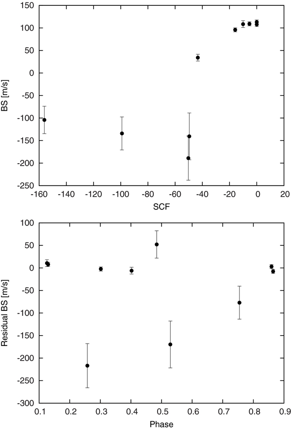
Figure 5. Top panel: the expected BS variation due to sky contamination (SCF) compared to the observed variation. The correlation between these values indicates that the observed BS variation for this relatively faint target appears to be due to contamination from scattered moonlight. Bottom panel: the residual BS variation when corrected for the SCF, compared to orbital phase. See Section 3.2.
Download figure:
Standard image High-resolution image3.3. Global Modeling of the Data
This section describes the procedure we followed to model the HATNet photometry, the follow-up photometry, and the radial velocities simultaneously. Our model for the follow-up light curves used analytic formulae based on Mandel & Agol (2002) for the eclipse of a star by a planet, with limb darkening being prescribed by a quadratic law. The limb-darkening coefficients for the Sloan i band were interpolated from the tables by Claret (2004) for the spectroscopic parameters of the star as determined from the SME analysis (Section 3.1). The transit shape was parameterized by the normalized planetary radius p ≡ Rp/R⋆, the square of the impact parameter b2, and the reciprocal of the half-duration of the transit ζ/R⋆. We chose these parameters because of their simple geometric meanings and the fact that these show negligible correlations (see Bakos et al. 2010; Kipping 2010). Our model for the HATNet data was the simplified "P1P3" version of the Mandel & Agol (2002) analytic functions (an expansion in terms of Legendre polynomials), for the reasons described in Bakos et al. (2010). Following the formalism presented by Pál (2009a), the RVs were fitted with an eccentric Keplerian model parameterized by the semi-amplitude K and Lagrangian elements k ≡ ecos ω and h ≡ esin ω, in which ω is the longitude of periastron.
We assumed that there is a strict periodicity in the individual transit times. We assigned the transit number Ntr = 0 to the first complete follow-up light curve gathered on 2010 January 1. The adjustable parameters in the fit that determine the ephemeris were chosen to be the time of the first transit center observed with HATNet, Tc, −129, and that of the last transit center observed with the FLWO 1.2 m telescope, Tc, 0. We used these as opposed to period and reference epoch in order to minimize correlations between parameters (see Pál et al. 2008). Times of mid-transit for intermediate events were interpolated using these two epochs and the corresponding transit number of each event, Ntr. The eight main parameters describing the physical model were thus Tc, −129, Tc, 0, Rp/R⋆, b2, ζ/R⋆, K, k ≡ ecos ω, and h ≡ esin ω. Three additional parameters were included that have to do with the instrumental configuration. These are the HATNet blend factor Binst, which accounts for possible dilution of the transit in the HATNet light curve from background stars due to the broad PSF (20'' FWHM), the HATNet out-of-transit magnitude M0, HATNet, and the relative zero-point γrel of the Keck RVs.
We extended our physical model with an instrumental model that describes brightness variations caused by systematic errors in the measurements. This was done in a similar fashion to the analysis presented by Bakos et al. (2010). The HATNet photometry has already been EPD- and TFA-corrected before the global modeling, so we only considered corrections for systematics in the follow-up light curves. We chose the "ELTG" method, i.e., EPD was performed in "local" mode with EPD coefficients defined for each night, and TFA was performed in "global" mode using the same set of stars and TFA coefficients for all nights. The five EPD parameters were the hour angle (representing a monotonic trend that changes linearly over time), the square of the hour angle (reflecting elevation), and the stellar profile parameters (equivalent to FWHM, elongation, and position angle of the image). The functional forms of the above parameters contained six coefficients, including the auxiliary out-of-transit magnitude of the individual events. The EPD parameters were independent for both nights, implying 12 additional coefficients in the global fit. For the global TFA analysis we chose 20 template stars that had good quality measurements for all nights and on all frames, implying an additional 20 parameters in the fit. Thus, the total number of fitted parameters was 11 (physical model with 3 configuration-related parameters) + 12 (local EPD) + 20 (global TFA) = 43, i.e., much smaller than the number of data points (322, counting only RV measurements and follow-up photometry measurements).
The joint fit was performed as described in Bakos et al. (2010). We minimized χ2 in the space of parameters by using a hybrid algorithm, combining the downhill simplex method (AMOEBA; see Press et al. 1992) with a classical linear least-squares algorithm. Uncertainties for the parameters were derived applying the Markov chain Monte Carlo method (MCMC; see Ford 2006) using the same method as Bakos et al. (2010). This provided the full a posteriori probability distributions of all adjusted variables. We assumed uniform prior probability distributions for each of the jump parameters. The Fisher covariance matrix was calculated analytically using the partial derivatives given by Pál (2009a).
Following this procedure, we obtained the a posteriori distributions for all fitted variables and other quantities of interest such as a/R⋆. As described in Section 3.1, a/R⋆ was used together with stellar evolution models to infer a theoretical value for log g⋆ that is significantly more accurate than the spectroscopic value. The improved estimate was in turn applied to a second iteration of the SME analysis, as explained previously, in order to obtain better estimates of Teff⋆ and [Fe/H]. The global modeling was then repeated with updated limb-darkening coefficients based on those new spectroscopic determinations. The resulting geometric parameters pertaining to the light curves and velocity curves are listed in Table 5.
Table 5. Orbital and Planetary Parameters
| Parameter | Value |
|---|---|
| Light curve parameters | |
| P (days) ... | 3.652836 ± 0.000019 |
| Tc (BJD)a ... | 2455176.85173 ± 0.00047 |
| T14 (days)a ... | 0.1174 ± 0.0017 |
| T12 = T34 (days)a ... | 0.0163 ± 0.0018 |
| a/R⋆ ... | 10.46+0.38− 0.55 |
| ζ/R⋆ ... | 19.75 ± 0.19 |
| Rp/R⋆ ... | 0.1275 ± 0.0024 |
| b2 ... | 0.208+0.075− 0.073 |
| b ≡ acos i/R⋆ ... | 0.456+0.073− 0.098 |
| i (deg) ... | 87.6 ± 0.5 |
| Limb-darkening coefficientsb | |
| ai (linear term) ... | 0.3287 |
| bi (quadratic term) ... | 0.3039 |
| RV parameters | |
| K ( m s−1) ... | 74.3 ± 2.4 |
| kRVc ... | 0.008 ± 0.012 |
| hRVc ... | −0.020 ± 0.034 |
| e ... | 0.032 ± 0.022 |
| ω (deg) ... | 271 ± 117 |
| RV jitter ( m s−1) ... | 3.5 |
| Secondary eclipse parameters | |
| Ts (BJD) ... | 2455178.698 ± 0.027 |
| Ts, 14 ... | 0.1138 ± 0.0060 |
| Ts, 12 ... | 0.0154 ± 0.0018 |
| Planetary parameters | |
| Mp (MJ) ... | 0.567 ± 0.022 |
| Rp (RJ) ... | 1.190+0.081− 0.056 |
| C(Mp, Rp)d ... | 0.15 |
| ρp ( g cm−3) ... | 0.42 ± 0.07 |
| log gp (cgs) ... | 3.00+0.04− 0.06 |
| a (AU) ... | 0.0466 ± 0.0005 |
| Teq (K) ... | 1202 ± 36 |
| Θe ... | 0.044 ± 0.003 |
| 〈F〉 (108 erg s−1 cm−2)f ... | 4.72 ± 0.58 |
Notes. aTc: reference epoch of mid-transit that minimizes the correlation with the orbital period. It corresponds to Ntr = −6. BJD is calculated from UTC. T14: total transit duration, time between first to last contact; T12 = T34: ingress/egress time, time between first and second, or third and fourth contact. bValues for a quadratic law, adopted from the tabulations by Claret (2004) according to the spectroscopic (SME) parameters listed in Table 4. cThe Lagrangian orbital parameters derived from the global modeling and primarily determined by the RV data. dCorrelation coefficient between the planetary mass Mp and radius Rp. eThe Safronov number is given by Θ = 1/2(Vesc/Vorb)2 = (a/Rp)(Mp/M⋆) (see Hansen & Barman 2007). fIncoming flux per unit surface area, averaged over the orbit.
Download table as: ASCIITypeset image
Included in this table is the RV "jitter." This is a component of assumed astrophysical noise intrinsic to the star that we added in quadrature to the internal errors for the RVs in order to achieve χ2/dof = 1 from the RV data for the global fit. Auxiliary parameters not listed in the table are Tc, −129 = 2454727.55286 ± 0.00233 (BJD), Tc, 0 = 2455198.76874 ± 0.00050 (BJD), the blending factor Binstr = 0.84 ± 0.06, and γrel = 13.5 ± 1.8 m s−1. The latter quantity represents an arbitrary offset for the Keck RVs and does not correspond to the true center-of-mass velocity of the system, which was listed earlier in Table 4 (γRV).
The planetary parameters and their uncertainties can be derived by combining the a posteriori distributions for the stellar, light curve, and RV parameters. In this way, we find a mass for the planet of Mp = 0.567 ± 0.022 MJ and a radius of Rp = 1.190+0.081− 0.056 RJ, leading to a mean density ρp = 0.42 ± 0.07 g cm−3. Figure 6 shows the mass and radius of HAT-P-256 compared to those of other known TEPs. These and other planetary parameters are listed at the bottom of Table 5. We note that the eccentricity of the orbit is not significant: k = 0.008 ± 0.012, h = −0.020 ± 0.034 (e = 0.032 ± 0.022, ω = 271° ± 117°).

Figure 6. Mass–radius diagram of known TEPs (small filled squares). HAT-P-25b is shown as a large filled square. Overlaid are Fortney et al. (2007) planetary isochrones interpolated to the solar equivalent semi-major axis of HAT-P-25b for ages of 1.0 Gyr (upper, solid lines) and 4 Gyr (lower, dashed-dotted lines) and core masses of 0 and 10 M⊕ (upper and lower lines, respectively), as well as isodensity lines for 0.4, 0.7, 1.0, 1.33, 5.5, and 11.9 g cm−3 (dashed lines). Solar system planets are shown with open triangles.
Download figure:
Standard image High-resolution image4. DISCUSSION
We have presented the discovery of a new transiting planet, HAT-P-25b, and provided a precise characterization of its properties. HAT-P-25b is a fairly typical, moderately inflated ∼0.5 MJ planet, similar in mass, radius, and equilibrium temperature to HAT-P-1b (Bakos et al. 2007b), WASP-25b (Enoch et al. 2011), and WASP-34b (Smalley et al. 2011). With V = 13.19, HAT-P-25 stands out as one of the faintest transiting planet host stars discovered by a wide-field ground-based transit survey to date (the only other transiting planet host stars with V > 13.0 discovered by wide-field ground-based transit surveys are HAT-P-28 with V = 13.03, Buchhave et al. 2011; and TrES-5 with V = 13.72, Mandushev et al. 2011). The host star GJ 1214 (V = 15.1; Charbonneau et al. 2009) was discovered by the MEarth project (Irwin et al. 2009), which is a ground-based, wide-field survey, but different in that it targets M dwarfs that are typically brighter in the infrared. While faint by the standards of surveys such as HAT and WASP, there are more than 30 other known transiting planet host stars fainter than HAT-P-25, which have been found primarily by space-based surveys (CoRoT and Kepler) and narrow-field ground-based surveys (OGLE). Figure 7 shows the histogram of host-star V magnitudes separated by discovery mission type.

Figure 7. Histogram of host star V magnitudes. Cross-hatched blue: host stars of transiting planets discovered by ground-based, wide-field surveys. Filled gray: host stars of transiting planets discovered from space or by ground-based, narrow-field surveys. Filled red: HAT-P-25.
Download figure:
Standard image High-resolution image
HATNet operations have been funded by NASA grants NNG04GN74G, NNX08AF23G, and SAO IR&D grants. Work of G.Á.B. and J. Johnson were supported by the Postdoctoral Fellowship of the NSF Astronomy and Astrophysics Program (AST-0702843 and AST-0702821, respectively). G.T. acknowledges partial support from NASA grant NNX09AF59G. We acknowledge partial support also from the Kepler Mission under NASA Cooperative Agreement NCC2-1390 (PI: D. W. Latham). G.K. thanks the Hungarian Scientific Research Foundation (OTKA) for support through grant K-81373. This research has made use of Keck telescope time granted through NOAO (A201Hr), NASA (N018Hr and N167Hr), and the NASA Gemini-Keck time-exchange program (G329Hr). This research has also made use of the NASA/IPAC Infrared Science Archive, which is operated by the Jet Propulsion Laboratory, California Institute of Technology, under contract with the National Aeronautics and Space Administration.
Footnotes
- *
Based in part on observations obtained at the W. M. Keck Observatory, which is operated by the University of California and the California Institute of Technology. Keck time has been granted by NOAO (A201Hr), NASA (N018Hr and N167Hr), and the NASA Gemini-Keck time-exchange program (G329Hr). Based in part on observations made with the Nordic Optical Telescope, operated on the island of La Palma jointly by Denmark, Finland, Iceland, Norway, and Sweden, in the Spanish Observatorio del Roque de los Muchachos of the Instituto de Astrofisica de Canarias.
- 10