


ABSTRACT
Quasi-regular timing observations obtained, using the 26 m Hartebeesthoek Radio Astronomy Observatory radiotelescope near center frequencies of 1.668 and 2.272 GHz, between 1985 July and 2005 August have given a further insight into the long-term spin-down behavior of the pulsar J1001−5507 (B0959−54). Here, we show that the spin-down of the pulsar during ∼20 years is dominated by dual spin-down modes characterized by two discrete and nearly stable spin-down rates ( s−2 and
  s−2). Our analysis demonstrates that the switching of the pulsar's spin-down rate from
  to
to  modes occurred over about 800 days (between about MJD 48500 and MJD 49300) at a steady rate of ∼−4.6 × 10⁻²⁴ s−3, after which the pulsar was found to be slowing down 1.3% faster. It is observed that the extreme pulse profile shapes at the two spin-down modes are notably different, while the interval of steady switching between the spin-down modes is coincident with evidence for some correlated pulse shape variations. We discuss these results in light of the current understanding of various mechanisms for radio pulsar spin-down modulation.
Export citation and abstract BibTeX RIS
1. INTRODUCTION
Rotation-powered pulsars (rapidly rotating, highly magnetized neutron stars) are expected to spin down steadily as their rotational kinetic energy is converted to electromagnetic radiation and high-energy particle accelerators. To a good approximation, the spin-down follows a simple power-law relation of the form (e.g., Manchester & Taylor 1977)

where ν and  are the pulsar spin frequency and its first time derivative, respectively; K = f(B, I, R, α) is a function that absorbs the neutron star structural factors and will be referred to throughout this paper as the "torque function" (following Allen & Horvath 1997); and n is the torque braking index. In its explicit form, K is given by

where B and I are, respectively, the neutron star surface magnetic field and moment of inertia, R is the stellar radius, α is the angle between the magnetic and the spin axes of the neutron star, and c is the speed of light. In its simplest form, the widely used standard vacuum dipole spin-down model, K is taken to be an arbitrary positive constant and n = 3 (Manchester & Taylor 1977). Timing irregularities (observed as deviations from this simple spin-down model) have generally been attributed to imperfections in the pulsar clock and could have far-reaching implications for neutron star structure and dynamics and their long-term spin-down evolution (see, e.g., Lorimer & Kramer 2005 for an overview).
The first significant departure from this simple model was observed as a sudden discontinuous change (a "glitch") in the rotation of the Vela pulsar (Radhakrishnan & Manchester 1969). Shortly afterward, Boynton et al. (1972) showed that timing instability in most pulsars is significantly dominated by sustained random fluctuations ("timing noise") in the pulse phase and/or its time derivatives. This phenomenon is basically typified by unmodeled structures in the timing residuals after accounting for the pulsar deterministic spin-down and any resolved glitch event. To date, only about 300 glitches have been reported in ∼100, mostly young, radio pulsars (Espinoza et al. 2011), while the prevalence of timing noise activity among the known pulsar population has been fairly well established (Chukwude 2007; Hobbs et al. 2010, and references therein).
Lately, a combination of improved timing techniques and long span of timing data has allowed for a more precise description of some dominant aspects of the radio pulsar timing noise phenomenon. Specifically, the aspects of pulsar rotational fluctuations characterized by long-term quasi-periodic modulations in the rotation of few isolated pulsars, coincident with some evidence for correlated pulse profile shape variations, have been observed in unprecedented detail (Stairs et al. 2000; Shabanova et al. 2001; Chukwude et al. 2003). The evidence has been observed as strongly correlated changes in either the pulse shape parameter (Stairs et al. 2000) or the time offsets between dual-frequency pulse times of arrival (e.g., Shabanova et al. 2001; Chukwude et al. 2003). Despite some serious theoretical constraints, these observations have been widely linked to precession of neutron stars (Melatos 2000; Link & Epstein 2001; Jones & Andersson 2001; Akg n et al. 2006; Ng 2010). More recently, Chukwude & Urama (2010) have shown that the observed timing noise activity in most middle-aged pulsars is largely dominated by poorly understood microglitch events: small amplitude discrete jumps in pulsar rotation frequency and/or its derivative, which are characterized by variable signatures (see also Cordes & Downs 1985; D'Alessandro et al. 1995).
Perhaps a more striking aspect of radio pulsars' spin-down evolution is the observed large persistent increases (or offsets) in magnitudes of the spin-down rates ( ) coincident with the 1975 and 1989 glitches in the Crab pulsar (Lyne et al. 1993) and the 1990 glitch in PSR B1830−08 (Shemar & Lyne 1996). Basically, these offsets are seen to be permanent (showing no obvious recovery of
  toward the pre-event values) and involve fractional increases in
  of ∼ (2–8) × 10−4. An offset in the spin-down rate of a pulsar is now widely attributed to a permanent increase in the external braking torque (Franco et al. 2000, and references therein). However, the underlying mechanism for the torque growth remains an issue of vigorous debate (see Alpar & Pines 1993; Link & Epstein 1997; Link et al. 1998; Franco et al. 2000).
In this paper, we report a high time resolution observation of the spin-down evolution of the pulsar J1001–5507 on a timesacle of ∼20 yr. It is shown that the pulsar displays two significantly (∼1.3%) different spin-down modes. The interval of smooth transition between the two modes is coincident with substantial evidence for profile shape variations.
2. OBSERVATIONS
The timing observations of the pulsar J1001–5507 reported in this paper were made at Hartebeesthoek Radio Astronomy Observatory (HartRAO) between 1985 July and 2005 August. However, the HartRAO pulsar timing project was interrupted for about 400 days (1999 June–2000 August) during observatory system upgrade. Nonetheless the pulsar-observing hardware was unchanged after this hiatus. Observations were made at an average interval of ∼14 days at frequencies centered near either 1.668 or 2.272 GHz with a 26 m HartRAO radio telescope. Pulses were recorded with a single 10 MHz bandwidth receiver at both frequencies and no pre-detection de-dispersion hardware was implemented during the period. The expected dispersive pulse smearing at 1.668 and 2.272 GHz are about 2.3 and 0.9 ms, respectively. The effects of dispersive smearing were assumed constant and were basically subtracted in subsequent data processing. Detected pulses were smoothed with a 500 μs filter time constant, sampled at 287 μs intervals and integrated over 630 consecutive rotation periods (about 15 minutes). An integration was usually started at a particular second by synchronization to the station clock, which was derived from a hydrogen maser and was referenced to the Coordinated Universal Time via a Global Positioning System network. At HartRAO, three such online integrations were made during an observing session. The average signal-to-noise ratios (S/Ns) of typical integrated pulse profiles are ∼3.5 and 4.2 at 2.272 and 1.668 GHz, respectively.
Topocentric arrival times were extracted from the observations by fitting an analytical pulse model to the data in least-squares sense. At HartRAO, the appropriate model is a Gaussian function whose parameters were obtained from the pulse profile template, a high S/N profile constructed by aligning and accumulating a large number of high S/N observations. Two such templates, one for each observing frequency, were constructed for the pulsar J1001−5507. Details of HartRAO data acquisition and reduction are described in Flanagan (1995).
3. DATA ANALYSIS AND RESULTS
3.1. Timing Analysis and Results
Subsequent data analyses were accomplished with TEMPO2 pulsar timing analysis software (Hobbs et al. 2006) and the HartRAO in-house timing analysis software (Flanagan 1995), which are based on the standard pulsar timing technique (e.g., Manchester & Taylor 1977). The topocentric pulse times of arrival were transformed to the barycenter of the solar system using the Jet Propulsion Laboratory DE200 solar system ephemeris. The resulting barycentric pulse times of arrival (BTOAs) were fitted with a simple spin-down model of the pulsar rotation frequency (ν) and its first and second time derivatives ( and
and  , respectively) of the form:

where ϕ0 is the pulse phase at an arbitrary time t0.
As is convention in pulsar timing, the observed BTOAs were compared with those predicted by the spin-down model to obtain the timing residuals. The timing residuals (δt), defined in the sense of the best model-predicted minus observed BTOAs, over a timespan of about 20 yr are shown in Figure 1(a). To obtain the pulsar's position and dispersion measure (DM), the BTOAs collected between MJD 48500 and MJD 49500 were first whitened to mitigate the effects of timing noise. The interval was chosen on the basis of its relative lower incidence of microglitch events (A. E. Chukwude 2011, in preparation). Following Hobbs et al. (2004), the whitening process was accomplished by modeling the timing residuals with four harmonically related sinusoids and then removing the function formed from the summation of these sinusoids from the BTOAs. The appropriate timing model was subsequently fitted to these whitened residuals. The resulting right ascension (R.A.) and declination (decl.), in J2000.0, are  and
and  , respectively. The DM is 130.5 ± 5 cm−3 pc, while the epoch of the measurements is MJD 48975.5. Our results are in good agreement with those from previous work (Siegman et al. 1993, hereafter SMD93). However, the presence of enhanced rotational instability is evident in the data. This resulted in peak-to-peak variations in the pulsar's BTOAs of ∼4000 ms. By implication, this translates to a loss of more than two complete pulse rotation phases over ∼20 yr. This is generally consistent with a positive average clock stability parameter, Δ8 > 0 recently reported for the pulsar (Chukwude 2007).
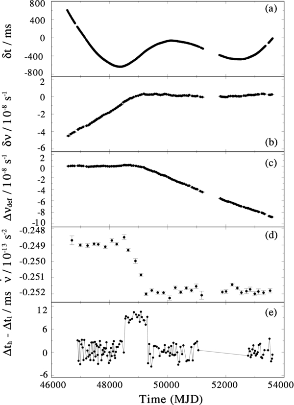
Figure 1. Evolution of the rotational parameters and BTOA time offsets for PSR J1001−5507 over ∼20 years. (a) Pulsar timing residuals (δt) relative to a simple spin-down model of ν,  and
and  . (b) Residuals of the pulse rotation frequency (δν(t)), obtained as described in the text. (c) Difference between the local and extrapolated values of the pulsar's rotation frequency (ν(t)) and νc0(t), respectively). (d) Variations of the pulsar's
  , obtained as described in the paper. Error bars are 1σ formal standard errors. (e) Time offsets between the BTOAs obtained at 1.668 and 2.272 GHz frequencies.
Download figure:
Standard image High-resolution imageTo investigate the nature of the pulsar's long-term spin-down evolution, it is necessary to examine the variations of its rotation frequency (ν) and spin-down rate ( ) with time over the ∼20 yr period. The local values of these parameters (ν(t) and
  ) were calculated by fitting a spin-down model of ν and
  to short, non-overlapping segments of BTOAs. The length of the segments is ∼50 days for ν(t), while it varied between 150 and 250 days for
  , depending on the density of observations and on our desire to keep the uncertainty below ∼0.1% of the parameter values. The frequency residuals (δν) relative to a spin-down model of ν and
  fitted to the entire ∼7000 day span of BTOAs, with epoch near the center, are plotted in Figure 1(b). Apparently, δν increased steadily from ∼−4 × 10⁻⁸ s−1 to zero at about MJD 49300, as the pulsar's
  increased from ∼0.249 × 10⁻¹³ to 0.252 × 10⁻¹³ Hz s−1. Thereafter,
  remained more or less stable and the frequency residuals appear randomly distributed about zero.
Furthermore, we calculated the deficit in the rotation frequency, Δνdef(t) = ν(t) − νc0(t): where ν(t) and νc0(t) are the local and the extrapolated values of the pulsar spin rate, respectively. Following Lohsen (1981), νc0(t) were estimated by referring the pulsar rotation frequency, obtained from a model [νc, ] fit to all pre-MJD 48500 BTOAs, to the epochs of the local values of the pulsar's ν. In this process, the spin-down rate
  Hz s−1 was held constant. It is expected that in the absence of appreciable systematic changes in
  , Δνdef(t) would be randomly distributed about zero. However, Figure 1(c) shows that subsequent to ∼MJD 48500 (the commencement of the steady increase in
  ), the magnitude of Δνdef started increasing steadily, and by 2005 August, the total cumulative offset peaked at ∼−10−7 Hz. As a check on the timing model, the frequency deficit was similarly calculated for the pulsar B0740−28, which exhibits a comparable level of rotational instability, though without systematic variations in
  (Chukwude 2003, 2007). In this case, the frequency deficit showed no discernible pattern, making it less probable that present observations could be mere artifacts of the timing model. The time variations of the pulsar's
  (resolved to ∼0.005 day−1) are plotted in Figure 1(d). Among other things, it shows that the pulsar's spin-down on long timescales has dual modes (corresponding to time intervals T < 48500 and T > 49300 MJD) characterized by two distinct and nearly stable spin-down rates. A model of ν and
  fitted to BTOA data between MJD 48000 and 48450 yielded
  s−2 (hereafter
  ). Between MJD 48500 and MJD 49300, (800 days)
  increased steadily at a rate of about −4.6 × 10⁻²⁴ s−3, culminating in about a −0.0032 × 10⁻¹³ s−2 (∼1.3%) permanent offset in
  . Beyond MJD 49300, the pulsar appears to have settled to a new spin-down mode characterized by
  s−2 (hereafter
  ), obtained by modeling BTOAs in the interval MJD 49500−MJD 49800. The observed offsets in the pulsar's rotation parameters are summarized in Table 1. These values of
  and
and  agree within 0.1% with the values obtained by simply averaging the pre-MJD 48500 and post-MJD 49300 local values of
  , respectively. Offsets in ν and
  were obtained by extrapolating the pre-MJD 48500 and post-MJD 49300 ephemeris to MJD 48500 (assumed epoch of commencement of the steady switch in
  ). The epoch uncertainty (ΔT) is < 100 days, (i.e., one half the length of segment used in calculating
  at MJD 48500). Although the amplitude of the pulsar's frequency offset (Δν) is sensitive to the assumed epoch, the change introduced by ΔT is within the limit of the quoted formal error. On the other hand, the size of the offset in
  (
( ) was found to be independent of ΔT.
Table 1. Parameters of the Offsets in the Rotational Parameters of the Pulsar J1001–5507
| Parameters | Values | |||
|---|---|---|---|---|
| Pre-MJD 48500 | Post-MJD 49300 | Offset | Size | |
| Frequency, ν (Hz) | 0.696093315928(8) | 0.696090234757(2) | Δν (10−6 (Hz)) | 0.0152(2) |
Frequency derivative,  (10−13 (Hz s−1)) (10−13 (Hz s−1)) |
−0.24871(3) | −0.25195(5) |  (10−13 Hz s−1) (10−13 Hz s−1) |
−0.00323(8) |
| Time interval fitted (MJD) | 48000–48450 | 49500–49800 | Δν/ν (10−6) | 0.024(10) |
| Rms phase residuals (ms) | 1.20 | 1.15 |  (10−2) (10−2) |
1.30(3) |
| Epoch (MJD) | 48229 | 49665 | 48500 |
Note. Uncertainties are 1σ standard error and refer to the least significant figure.
Download table as: ASCIITypeset image
3.2. Pulse Shape Change Analysis and Results
3.2.1. Pulse Arrival Time Offset Analysis
In addition to the long time coverage, the HartRAO timing observations on PSR J1001−5507 were more or less alternated between two frequencies centered around 1.668 and 2.272 GHz. The residuals of the BTOAs at the two observing frequencies (compare Figure 1(a)) reveal no apparent difference between the high- and low-frequency observations. However, a more rigorous analysis of the timing residuals was conducted by carefully comparing the arrival times of the pulses at 1.668 and 2.272 GHz. The BTOA residuals were divided into independent segments of length ∼40 days, such that each valid bin contains BTOAs at both frequencies. The BTOA residuals in each segment were then averaged separately. The time offsets, defined as the difference between the average values of the high- and low-frequency BTOA residuals, are shown in Figure 1(e). Save for the fairly large intrinsic scatter, the pre-MJD 48500 and post-MJD 49300 time offsets appear randomly distributed around zero. The plot, however, reveals that the pulse, on average, arrives ∼8.0 ms earlier at 1.668 GHz than at 2.272 GHz during the ∼800 day interval of steady increase in  .
.
3.2.2. Methods of Principal Component Analysis
Recently, Trangsrud (2003) published an in-depth overview of the application of the methods of principal component analysis (PCA) to probing radio pulsar data for long-term profile shape changes. The methods used by the author, including the accompanying FORTRAN code, are deployed in analysis in this paper. Basically, application of PCA involves construction of a weighted average pulse profile (hereafter WAPP) from a set of observations (the integrated pulse profiles), subtraction of the WAPP from the observations to obtain the profile residuals, and then rigorous computer analyses of the residuals for profile shape variations. Following Trangsrud (2003), the WAPP  is computed as
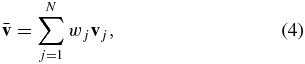
where v is an m-dimensional vector (m = number of bins in a profile), N is the number of integrated profiles, and wj is the weight assigned to jth profile  . The residuals of the jth profile are given by
  . The amplitudes of the jth component, which contribute appreciably to the residuals of the kth profile, are computed by (e.g., Trangsrud 2003; McDonald 2006)

where e is the eigenvector matrix and j = 1 (that is, a1) corresponds to the principal (first) component, which contributes most significantly to the residuals.
The database on current pulsar consists of about 890 and 1560 integrated pulse profiles (hereafter IPPs) recorded near center frequencies of 2.272 and 1.668 GHz, respectively. A typical IPP consists of ∼5000 samples spanning the 360° topocentric pulsar rotation period and S/N in the range of ∼2–7. The pulsar's pulse profile templates at 1.668 and 2.272 GHz are shown in Figure 2(a). The two extreme pulse profile shapes at 1.668 GHz corresponding to the two spin-down modes, characterized by  and
and  , are compared in Figure 2(b). It is shown that the extreme pulse profiles have moderately different shapes at the two spin-down modes. To quantitatively discriminate between the two profiles, we estimated their equivalent widths (Weq, defined as the area under the pulse divided by the peak amplitude). We found Weq ≃ 33.9 and 36.1 for the average profiles corresponding to
  and
and  , respectively, yielding a difference in the equivalent widths ΔWeq ≃ 2.2.

Figure 2. Integrated pulse profiles of the pulsar J1001−5507. (a) Typical pulse profile templates at 1.668 and 2.272 GHz, obtained by averaging over ∼1600 and 900 observations, respectively. (b) The two traces represent the most extreme profile shapes at 1.668 GHz corresponding to  mode (thin line) and
  mode (thick line). (c) Expanded version of panel (b) highlighting the ∼7% difference in the equivalent widths Weq of the extreme profiles at the pulsar's dual spin-down modes. All profiles are normalized to a unit height.
Download figure:
Standard image High-resolution imageA direct application of PCA to the IPPs has no chance of producing realistic results given the poor S/N of the data. It is imperative that we construct a set of new higher S/N profiles by combining the large sample of IPPs. Basically, we divided the IPPs into small segments of constant length Δτ = 100 days, where each segment contains 7–86 IPPs. The data in each segment were carefully aligned to obtain an averaged pulse profile normalized to unit height (hereafter AvPP). The epoch and S/N of each AvPP are the averages from the constituent IPPs. Data at the two observing frequencies were analyzed independently. The current averaging technique yielded 56 and 68 AvPPs at 2.272 and 1.668 GHz, respectively, whose S/Ns were improved by factors of ∼3–9. In addition, the current choice of Δτ appears to represent a good compromise between obtaining AvPPs with appreciable higher S/Ns and having a sizeable sample for meaningful principal component analyses.
A simple simulation analysis revealed that a realistic application of the PCA technique requires pulse profiles with S/N ≳ 10 (see also Trangsrud 2003). Consequently, only 46 and 56 AvPPs at 2.272 and 1.668 GHz, respectively, with S/N ≳ 8 were considered suitable for the PCA analysis. The weights assigned to the AvPPs were calculated from the S/Ns of the constituent IPPs. The number of samples in the AvPPs was scaled down to 500 centered at the pulse midpoint. This covers about 10% (∼145 ms) of the topocentric pulsar period and is about six times the object's pulse full widths at 10% of the maximum intensity (McCulloch et al. 1978). The PCA software weights the AvPPs linearly based on their estimated S/Ns. The scatter plots of the first component amplitudes (a1: which accounts for much of the variability in the data) for the 1.668 GHz data are shown in Figure 3(a) for the 56 AvPPs. The observed scatter in the data could be attributed to a combination of considerable dispersion (∼8–23) in the S/N of the AvPPs and modest profile shape changes. Nonetheless, there is an apparent downward trend in the data, in which a1, on average, decreases with time (T). A simple linear regression analysis yields a marginal a1–T correlation (with a correlation coefficient r ≃ −0.4). This, probably, suggests the existence of some form of regular time-dependent profile shape variations in the current data. We remark that the a1–T correlation improved to r ∼ −0.5 when data with S/N < 10 were excluded from the analysis.

Figure 3. Variations of the first component amplitude (a1) for 1.668 GHz AvPPs with time (a) and the spin-down rate ( ) (b). AvPPs in panel (a) were obtained from short chunks of IPPs of length Δτ = 100 days, while the AvPPs in panel (b) were obtained from short segments of data whose lengths are equal to those used to calculate the corresponding
  . Key: 3(b) • = for data up to about MJD 48500 (subsample I),
  = for data between ∼48500–49300 (subsample II), and ▴ = for data beyond ∼MJD 49300 (subsample III). Error bars are standard deviations of the AvPPs from the corresponding WAPPs.
Download figure:
Standard image High-resolution image
For further insight into the profile shape changes, we investigated the relationship between a1 and  . Again the IPPs at 1.668 GHz were divided into 34 segments of unequal lengths. The lengths of the segments were carefully selected to correspond exactly to those used to calculate
  in Section 3.1. The IPPs in the segments were similarly averaged, yielding 34 AvPPs with S/Ns in the range of ∼15–35. The new set of 34 AvPPs were divided into three subsamples I, II, and III corresponding to the pulsar's three distinct spin-down states. The subsample I (with 8 AvPPs) spans up to MJD 48500, while II and III (with 5 and 21 AvPPs, respectively) span MJD 48500−49300 and beyond MJD 49300, respectively. Thereafter, the data in I, II, and III were analyzed separately using the PCA technique. The resulting first component amplitudes are plotted against the corresponding spin-down rates in Figure 3(b). The plot reveals a strong
  correlation only within the interval of steady increase in
  (subsample II). We estimated errors in the component amplitudes by calculating the standard deviations of the AvPPs relative to the associated WAPPs. This is a simple method which might reasonably overestimate the uncertainties in a1, given that the pulsar's pulse profiles actually change, though moderately. Nonetheless, we believe that the result represents, at least, an upper limit on the parameter uncertainty.
The results of the eigenvectors' analysis and the second component amplitudes (a2) show no discernable feature above the level of uncorrelated data noise. It is equally worthy of note that similar applications of PCA to the 2.272 GHz pulse profile data gave results that are generally not distinguishable from the uncorrelated data noise. This is not unexpected given that the IPPs at this frequency have relatively lower S/Ns and are about half the size of the IPPs at 1.668 GHz. As a consequence, the AvPPs from chunks of 100 days are characterized by relatively lower S/Ns. We also remark that the poor S/N of the current data precluded a more direct analysis of the profile shape variations, using the pulse shape parameters (e.g., Stairs et al. 2000).
4. DISCUSSION
The pulsar J1001–5507 has a rotation period of ∼1430 ms and a typical spin-down rate of about 50 × 10−15 s s−1. Although it has been extensively monitored for glitches, no classical glitch has been resolved in the object as yet (e.g., Wang et al. 2000, and references therein). An analysis of Mount Pleasant Observatory timing data on the pulsar, with a time span of seven years, reveals remarkably smooth and seemingly oscillatory timing residuals. The residuals were found to be marginally anti-correlated with the odd moments of the 650 MHz integrated pulse profiles (D'Alessandro & McCulloch 1997). Several authors (e.g., Link & Epstein 2001; Jones & Andersson 2001; Cutler et al. 2003) have linked these results to a precessing neutron star with a long precession period Pp ≫ 2500 days (the time span of data used in the analysis by D'Alessandro & McCulloch 1997). Current analysis of ∼20 yr span of BTOAs, which completely overlap the Mount Pleasant Observatory data, could not confirm any quasi-periodic modulation in the pulsar rotation (at least on a timescale of ∼7000 days). It nonetheless reaffirms the existence of some form of regular variations in the pulsar's profile shapes.
The results of our analyses have, among other things, demonstrated that the observed structure in the timing residuals of the pulsar J1001–5507 is dominated by variations in its spin-down, which is bi-modal on long timescales with  s−2 and
  s−2. The smooth switching of the pulsar's spin-down between the two modes occurred over a period of ∼800 days at a constant rate of −4.6 × 10⁻²⁴ s−3. The observed peak amplitude change of ∼−5 × 10⁻⁸ s−1 in the frequency residuals (δν) prior to MJD 48500 is consistent with an offset of about 3.2 × 10⁻¹⁶ s−2 relative to the model value of
  s−2 used in our calculation. In particular, the cumulative frequency deficit, whose peak of ∼−1.0 × 10⁻⁷ s−1 occurred at about MJD 53500, suggests that the pulsar was actually rotating progressively less rapidly following the commencement of the event at ∼MJD 48500.
We find that the extreme pulse profiles at 1.668 GHz are modestly (6.5%) different at the pulsar's two extreme spin-down modes ( and
and  ). In addition, the first component amplitude (a1) of these profiles, though reasonably contaminated by uncorrelated data noise, is significantly anti-correlated (with r ∼ −0.5) with time. The results become more interesting when the analysis is broken down into the different states of the pulsar's spin-down (compare Figure 3(b)). Perhaps the most striking feature in the plot is the strong
  correlation (with a correlation coefficient r ≃ 0.97) obtained during the interval of steady increase in
  (subsample II). By contrast, there is no apparent
  relation during the two extreme spin-down modes characterized by nearly stable
  and
and  (subsample I and III, respectively). Nonetheless, a1 appears to be appreciably different, at least on average, for the two modes. Specifically, we find a1 = −0.46 ± 0.05 and 0.15 ± 0.06 (where errors are 1σ standard error in mean) for
  and
and  modes, respectively. This is consistent with the object's pulse profile shapes being modestly different for the two spin-down modes. Current results suggest that the variations in the pulsar's profile shapes are regular during the episode of transition between the two spin-down modes. This view is, in principle, supported by the ∼ 8.0 ms time offset between the 2.272 and 1.668 GHz BTOAs seen during the interval. In addition, the profile shapes, though only marginally different for the two spin-down modes, do not vary systematically as long as the pulsar's
  is more or less stable. The moderate evidence for regular profile shape variations seen in all the 1.668 GHz data (cf. Figure 3(a)) could be traced to the WAPP, which was constructed from all the observations. Given that the interval of steady increase in
  (during which the profile shapes are believed to vary in a regular pattern) accounts for ∼10% of all the data, the WAPP shapes would differ only marginally and more or less systematically from the IPPs. This probably would produce component amplitudes that are barely above the noise level in the data, hence accounting for the observed marginal a1–T anti-correlation.
In principle, an increase in  could arise from an increase in the pulsar's torque function (K) or braking index (n). An increase in K could result from a decrease in the effective moment of inertia acted upon by the external braking torque. This could occur through either a structural change—e.g., the star becomes less oblate as it spins down—or a decoupling of a portion of the neutron superfluid component from the inner stellar crust (Baym & Pines 1971; Alpar & Pines 1993). In this case, conservation of angular momentum would cause the pulsar to spin up progressively, requiring that ν < νc0 following the 1991 event (see, e.g., Link et al. 1992, 1998; Link & Epstein 1997). However, that ν − νc0 < 0 following the event implies that the pulsar was caused to spin less rapidly than it would have had the event not occurred. Moreover, such simple structural changes cannot plausibly account for the observable changes in the shape of the pulse profiles. An alternative interpretation of the observed switch in
  in terms of a transient permanent increase in the neutron star magnetic dipole moment (m = BR3/2: where B and R are the surface magnetic field strength and radius of the neutron star, respectively) is equally severely constrained. While a gradual growth in B, probably through a method of rapid magnetization is not completely ruled out in pulsars, such a process is unlikely to be important in a pulsar with a relatively large characteristic age (see, e.g., Michel 1994; Muslimov & Page 1995, 1996). Moreover, it is difficult to accommodate such an intermittent large amplitude switch in the pulsar spin-down rate in any existing model for growth in B.
Perhaps an attractive interpretation of the observed switch in  is in terms of a persistent steady increase in the angle α between the pulsar spin and magnetic axes. This scenario has been particularly successful in explaining some aspects of the observed Crab pulsar spin behavior (e.g., about 0.04% persistent increase in
  and a cumulative rotation frequency deficit) following the relatively large glitch events of 1975 and 1989 (Link et al. 1992, 1998; Link & Epstein 1997; Franco et al. 2000). Link & Epstein (1997) posited that the large fractional increase in the Crab pulsar spin-down rate, coincident with the 1989 glitch event, could cause measurable changes in the shape of the pulsar integrated pulse profiles. Incidentally, there have been some reports of ∼60 s periodic modulation in the Crab pulsar optical pulse profile data (C˘adez˘ et al. 1997, 2001). However, the origin of this variation has remained largely speculative (e.g., Lorimer & Kramer 2005, and references therein).
A change in the angle between pulsar spin and magnetic axes would cause variations in the external braking torque acting on the pulsar. In theory, the nature of the external torque variation, as reflected by the time evolution of  , would depend on the manner of the change in α. While a cyclic variation is expected to produce a quasi-periodic modulation of the observed spin-down rate (Stairs et al. 2000; Shabanova et al. 2001; Chukwude et al. 2003), a steady permanent increase in α would result in a permanent offset in
  (Link et al. 1992; Link & Epstein 1997). Accordingly, the pulsar would be rotating progressively more slowly, causing a cumulative rotation frequency deficit (Link et al. 1992, 1998). The ∼1.3% cumulative fractional increase in the spin-down rate of the pulsar over about an 800 day period suggests a fractional growth rate of ∼1.668 × 10⁻³ day−1. In the context of the vacuum dipole model for pulsar spin-down, the angle α will increase at a rate
  day−1. The growth in α will be cumulative in nature and for the mean segment length of about 200 days used in calculating
  , α could increase to ∼0
 3 (assuming α = 60°). This value could be significantly larger if the pulsar has approached an orthogonal rotator. Such an amplitude change in α could induce measurable shape changes in the pulsar pulse profiles. We posit that the marginal evidence for pulse shape variation reported by D'Alessandro & McCulloch (1997) has its origin in the event observed between MJD 48500 and MJD 49300 during which the pulsar steadily and slowly switched between two distinct spin-down states.
An increase in the external braking torque acting on an isolated pulsar could originate from plate tectonic activity (Ruderman 1970, 1991) in which stresses exerted on the stellar crust by pinned superfluid vortices crack the crust and drag crustal plates toward the equator. In principle, stress could easily build up from the differential rotation between the crust and the interior neutron superfluid as the pulsar spins down. The surface magnetic field, which is frozen to the crust, moves with crustal plates increasing the angle α between the dipole moment and the spin axes of the star (Link et al. 1992). Similarly, starquakes—occurring as a star slows down and becomes less oblate—have a finite probability of increasing the braking torque on an isolated, rapidly slowing pulsar (Baym & Pines 1971; Link & Epstein 1997). Starquake activity, among other things, causes an asymmetric re-distribution of the neutron star matter. This has the tendency of exciting damped precession, which could permanently increase α. The relatively large spin-down rate of the current pulsar J1001−5507 ( s s−1) suggests that starquakes could still play an important role in its spin-down evolution.
While completing this work, we became aware of a novel paper by Lyne et al. (2010), which linked many observed pulsar phenomena to changes in the magnetosphere. Specifically, the authors demonstrate that most hitherto observed pulse profile shape changes that accompany variations in pulsar spin-down rates arise from changes in the states of the magnetosphere rather than from free precession. The bottom line is that timing activity is predicated on changes in the pulsar emission properties (see also Kramer et al. 2006). Some striking similarities between the current result and that presented in Lyne et al. (2010)—the existence of two significantly (∼1.3%) different discrete spin-down rates and oscillatory, asymmetric timing residuals—also make the magnetospheric variation model a possible explanation of current observations of PSR J1001−5507.
4.1. Comparison with Previous Work
The results from seven pulsars whose spin-down behaviors are coincident with long-term pulse shape variations (Lyne et al. 2010) are compared with current results on PSR J1001−5507 in Table 2. Our results are generally in good agreement with those published by the authors. However, the similarities between the spin-down behavior of the current pulsar and J2037+3621 are so striking that few comments are necessary. The long-term spin-down history of the two pulsars shows dual spin-down modes, characterized by more or less stable low and high  (
( and
and  , respectively). The switching from
  to
to  is remarkably linear and occurs at similar timescales in both pulsars. Lomb–Scargle spectrum analyses of the pulsars'
  show that the timescales of spin-down variations are of the same order of magnitude (≳ 20 yr).
Table 2. Measured Parameters of PSR J1001–5507 as Well as 7 Pulsars Shown by Lyne et al. (2010) to Exhibit Significant Pulse Profile Shape Changes
| Pulsar | Pulsar | ν |  |
 |
F | Comment |
|---|---|---|---|---|---|---|
| Bname | Jname | (H) | (10−15 Hz s−1) | (%) | (yr−1) | |
| B1931+24 | J1933+2421 | 1.229 | −12.25 | 44.90 | 13.1(7) | Intermittent pulsar |
| B2035+36 | J2037+3621 | 1.616 | −12.05 | 13.28 | 0.02(2) | 28% change in Weq |
| B2043+2740 | J2043+2740 | 1.543 | −11.76 | 6.80 | 0.36(13) | 100% change in W50 |
| B1822−09 | J1825−0935 | 1.300 | −88.31 | 3.28 | 0.40(7) | 100% change in Apc/Amp |
| B1540−06 | J1543−0620 | 1.410 | −1.75 | 1.71 | 0.24(2) | 12% change in W10 |
| B0959−54 | J1001−5507 | 0.696 | −24.88 | 1.30 | 0.055(10) | 6.5% change in Weq |
| B1828−11 | J1830−1059 | 2.469 | −365.68 | 0.71 | 0.73(2) | 100% change in W10 |
| B0740−28 | J0742−2822 | 5.996 | −604.36 | 0.66 | 2.70(20) | 20% change in W75 |
Notes. We list the parameters in this order: pulsar names, spin frequency, spin-down rate, peak-to-peak fractional change in  , fluctuation frequencies F of the peaks of the Lomb–Scargle power spectra of the spin-down rates. The values in parentheses are the widths of the peaks or groups of peaks in units of the last quoted digit.
Download table as: ASCIITypeset image
The observed long-term variations in the pulse profiles of both objects are remarkably similar in many aspects. For instance, the extreme pulse profiles at the two nearly stable spin-down modes are significantly different. Quantitatively, the profile corresponding to the largest  has a smaller Weq for both pulsars. The modest change in Weq reported in this paper appears consistent with the relatively smaller amplitude change in the spin-down rate of PSR J1001−5507. It is worthy of note that the size of the profile changes is strongly dependent on the amplitude change in the pulsars'
  . It is expected that small amplitude changes in a pulsar's
  will cause equally small changes in its emission beam which crosses the line of sight to the Earth, leading to moderate profile variations. In particular, we find
  . A combination of modest profile changes and poor S/N precluded a more direct analysis of profile shape changes on a timescale of
  in the current data set. However, an indirect probe of the profile variations using the component amplitudes shows that variations in the pulsar's profiles are strongly correlated with
  during the interval of steady switching between the bi-modal spin-down states, in excellent agreement with the result on PSR J2037+3621 (Lyne et al. 2010).
5. CONCLUSION
We have demonstrated that the long-term spin-down history of the pulsar J1001−5507 displays two distinct spin-down modes characterized by  s−2 and
  s−2. The switch from
  to
to  took ∼800 days and occurred at a rate of −4.6 × 10⁻²⁴ s−3. The transition between the pulsar's dual spin-down modes is found to be coincident with some observations (∼8.0 ms offset between BTOAs at 1.668 and 2.272 GHz, a very strong
  correlation for the 1.668 GHz pulse profiles) suggestive of some pulse profile shape variations. We interpret current results in terms of changes in the angle between the neutron star spin and magnetic axes, but note that changes in the pulsar magnetosphere are equally plausible.
This work was done in part while A.E.C. was on a short postdoctoral research visit to HartRAO. He is grateful to the Directors and staff of both HartRAO and the Johannesburg Planetarium for their financial support and hospitality during his visit.