


ABSTRACT
We present the results of an extensive survey of RR Lyrae (RRL) stars in three fields along the major axis of the Triangulum Galaxy (M33). From images taken with the Advanced Camera for Surveys (ACS) Wide Field Channel on board the Hubble Space Telescope through two passbands (F606W and F814W), we have identified and characterized a total of 119 RRL variables (96 RRab (RR0) and 23 RRc (RR1)) in M33. Using the properties of 83 RRL stars (65 RRab and 18 RRc) in the innermost ACS field (hereafter DISK2), we find mean periods of 〈Pab〉 = 0.553 ± 0.008 (error1) ± 0.05 (error2) and 〈Pc〉 = 0.325 ± 0.008 (error1) ± 0.05 (error2), where the "error1" value represents the standard error of the mean and the "error2" value is based on the error of an individual RRL period calculated from our synthetic light curve simulations. The distribution of RRab periods and the frequency of RRc stars (Nc = nc/nabc = 0.22) strongly suggest that these RRLs follow the general characteristics of those in Oosterhoff type I Galactic globular clusters. The metallicities of 65 individual RRab stars are calculated from the period–amplitude–metallicity relationship, yielding a mean metallicity of 〈[Fe/H]〉 = −1.48 ± 0.05 dex, where the uncertainty is the standard error of the mean. The VI minimum-light colors of the RRab stars are used to calculate a mean line-of-sight reddening toward the DISK2 field of 〈E(V − I)〉 = 0.175. By adopting this line-of-sight reddening and using a relation between RRL luminosity and metallicity (MV = 0.23[Fe/H]+0.93), we estimate a mean distance modulus of 〈(m − M)0〉 = 24.52 ± 0.11 for M33, where the error is the quadratic sum of the uncertainties in the absolute and dereddened V magnitudes of the RRLs. The Oosterhoff I properties of the M33 field RRL stars agree well with those of RRL populations found in the M31 halo consistent with the past interaction history of these two galaxies.
Export citation and abstract BibTeX RIS
1. INTRODUCTION
In the Local Group, the Triangulum galaxy, M33, is the third most massive galaxy and is the only other spiral besides its giant cousins (the Milky Way (MW) and M31). Unlike its more massive counterparts, M33 has a late-type morphology (Scd) without a bulge (or a very weak bulge); the galaxy has a relatively low dark halo virial mass of ∼1011 M☉ (Corbelli 2003) and a high total gas mass fraction of 0.2–0.4, which is at least two times higher than that in M31 (Garnett 2002; Corbelli 2003). The late-type spiral galaxy M33 has not been studied as extensively as the MW and M31. The measured distance to M33 shows a large dispersion (730 ∼ 970 kpc) in the literature and is still controversial, mainly due to the uncertainty in the reddening values. The star formation history throughout several different parts of M33 (inner disk and outer disk/halo) was recently studied by Barker et al. (2007) and Williams et al. (2009). The results in the literature are quite intriguing. While the inner part (rgc < 7 kpc) of the galaxy shows the signature of inside-out growth (Williams et al. 2009), the outer part (rgc > 7 kpc) shows an increase in the age of the stellar population with galactocentric distance (Barker et al. 2007). Large numbers of globular cluster (GC)-like objects have been found in M33. The GC system in M33 appears to have a very broad range of ages exhibiting a stronger resemblance to the cluster populations of the lower-mass Magellanic Clouds than the MW or M31 (Sarajedini et al. 2000; Chandar et al. 2002; Sarajedini & Mancone 2007; San Roman et al. 2009). Recently, Huxor et al. (2009) discovered four remote star clusters in the outer halo of M33. By comparing the (V − I) colors of the new clusters to the MW and M31 outer halo GCs, they concluded that the M33 halo clusters are archetypical GCs as well. The existence of the field halo RR Lyrae (RRL) population was confirmed by the pioneering work of Sarajedini et al. (2006, Paper I). They found the mean period of ab-type RRL (RRab) stars to be 〈Pab〉 = 0.54 days, which is consistent with the mean period of M31 halo RRLs and RRLs in Oosterhoff type I MW globular clusters. The ab-type RRL stars are fundamental mode pulsators, which exhibit sawtooth-like light curves, whereas c-type RRL (RRc) stars are first overtone pulsators with light curves that are sinusoidal. The presence and characteristics of those RRLs provide direct evidence supporting the notion that the M33 halo contains a significant old population (>10 Gyr).
In this paper, we focus on the RRL population in M33 using new space-based observations. This population is a versatile tool; a wide range of astrophysical questions can benefit from the study of these stars. RRL stars are a well-known population II standard candle used to provide an accurate distance to M33. In addition, the (V − I)0 minimum light color is well established so that it can be used to accurately determine the line-of-sight reddening toward each RRL in M33. The pulsation periods and amplitudes of RRab exhibit a relationship with metallicity. By combining knowledge of their old ages (>10 Gyr), we can constrain age and metallicity information in the early stages of M33's formation. This paper is organized as follows. In Section 2, we describe the observations and data reduction procedure. In Section 3, we present the detailed procedure used to select and characterize the RRL candidates. We present the synthetic light curve simulations and the results in Section 4. The radial trends in the metallicity of our RRL candidates and their implications for the formation of the M33 halo are discussed in Section 5. Finally, in Section 6, we summarize our results and present the conclusions of this study.
2. OBSERVATIONS AND DATA REDUCTION
The science images used in this study were taken along the major axis of M33 with the Advanced Camera for Surveys Wide Field Channel (ACS/WFC) on board Hubble Space Telescope (HST) as a part of the GO-10190 program (P.I.: D. Garnett). The observations were originally intended to study the star formation history of the M33 disk. We used three primary ACS/WFC fields in the southwest direction referred to as "DISK2" (r = 9 3), "DISK3" (r = 159), and "DISK4" (r = 226) for the present survey of RRL stars, where r represents the galactocentric distance of each target field in arcmin. For each target field, 20 exposures through the F606W and 24 exposures through the F814W were taken. The observing log is summarized in Table 1.
Table 1. Observing Log
| Field | R.A. (J2000) | Decl. (J2000) | Filters | Exp. Time | Data Sets | HJD Range (+2 450 000) |
|---|---|---|---|---|---|---|
| DISK2 | 01 33 39.69 | +30 28 59.98 | F606W | 16 × 1240 s, | j90o21,j90o23 | 3257.10472 to 3260.25101 |
| 2 × 650 s, 2 × 60 s | ||||||
| F814W | 20 × 1240 s, | j90o24,j90o26 | 3258.10428 to 3258.85153 | |||
| 2 × 750 s, 2 × 60 s | ||||||
| DISK3 | 01 33 20.49 | +30 22 14.99 | F606W | 16 × 1240 s, | j90o31,j90o33 | 3416.70446 to 3416.85083 |
| 2 × 650 s, 2 × 60 s | 3418.70294 to 3418.84935 | |||||
| 3421.63415 to 3421.78837 | ||||||
| F814W | 20 × 1240 s, | j90o34,j90o36 | 3386.71436 to 3386.93625 | |||
| 2 × 750 s, 2 × 60 s | 3414.70627 to 3414.85230 | |||||
| 3421.10114 to 3421.31423 | ||||||
| DISK4 | 01 33 07.89 | +30 15 06.98 | F606W | 16 × 1240 s, | j90o41,j90o43 | 3314.61986 to 3320.16401 |
| 2 × 650 s, 2 × 60 s | ||||||
| F814W | 20 × 1240 s, | j90o44,j90o46 | 3313.96950 to 3319.43119 | |||
| 2 × 750 s, 2 × 60 | ||||||
Download table as: ASCIITypeset image
The raw images of these three target fields were processed by the standard STScI pipeline (bias and dark subtracted, and flat fielded); these calibrated "FLT" images were downloaded from the HST archive. In order to prepare the program FLT images, which were used for the point-spread function (PSF) photometry, we first multiplied them by the corresponding geometric correction frames; the bad pixels were masked by applying the data-quality files and the PSF photometry was performed on the resulting frames of each ACS chip (WFC1 and WFC2) using the DAOPHOT/ALLSTAR and ALLFRAME routines (Stetson 1994). A detailed description of the PSF construction and the time-series photometry is presented in Sarajedini et al. (2006). The effect of a decreasing charge transfer efficiency (CTE) for WFC was corrected on the resulting photometry by using the ACS/CTE characterization devised by Riess & Mack (2004). Then, the photometric calibration of the instrumental magnitudes to the standard Johnson–Cousins system was performed via the theoretical transformation of Sirianni et al. (2005). We adopted the latest ACS zero-point values, which were revised on 2009 May 19 (ACS ISR 07-02).
The resulting photometry reaches V ∼29.5 mag (see Figure 1). The average photometric accuracy at the level of the horizontal branch and the red clump of M33 is 〈σ〉 ∼ 0.05 mag. Therefore, we do not expect photometric accuracy to adversely affect the remaining analysis of the RRLs.

Figure 1. Location of the RRL candidates in the (V, V − I) CMDs of the three ACS fields (DISK2, DISK3, DISK4). Most RRL candidates are located in the instability strip between the blue edge of this strip (dotted blue line, (V − I)0,BE = 0.28; Mackey & Gilmore 2003) and the red clump stars (RCs) of M33. The slopes shown in the distribution of RRLs and RCs reflect the amount of reddening and extinction toward the target fields as shown by the vectors in each panel.
Download figure:
Standard image High-resolution image3. DETECTION OF RR LYRAE VARIABLE CANDIDATES
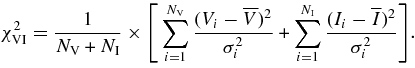
We attempt to detect all possible variable star candidates within a range of V magnitude (28 < V < 24) by calculating the reduced χ2VI value for measuring variability of each star which is defined by the following formula:
In order to avoid false variability due to odd photometric measurements, any data point that deviates from the mean magnitude by 3σ was excluded from the χ2VI calculation. Stars with a χ2VI value greater than 2.5 were considered to be variable star candidates. For reference, the reduced χ2VI value for a typical non-variable star at the magnitude of the RRLs in M33 (〈V(RR)〉 = 25.95 from Paper I) is ∼ 2.5. This variability criterion produced a list of about 2000 variable star candidates from the three ACS/WFC fields analyzed herein.
We applied our own light curve template-fitting routine dubbed, "FITLC" (Layden 1998; Mancone & Sarajedini 2008) to the F606W and F814W passband magnitudes of these variable star candidates in order to find the best combination of period and amplitude. The latest version of FITLC implements the Lomb–Scargle periodogram (Lomb 1976; Scargle 1982) module for the initial guess of the best possible periods. Then the final output periods and amplitudes are refined by running the "Pikaia" algorithm (Charbonneau 1995), which is a robust optimization routine that searches for the best combination of period and amplitude through a given range of test periods that minimizes the χ2P values between the observed data points and 10 different light curve templates (Layden 1998). In this case, χ2P represents the goodness of template fitting at the test periods for each RRL candidates. Stars with minimum χ2P less than 3.0 at the best-fitting period are considered probable RRL candidates. From our experience, this threshold is generous enough to include practically all potential RRL candidates. Finally, we examined the light curves of the probable RRL candidates to construct our final RRL list. We find 86 RRL stars from the DISK2 field (65 RRab, 18 RRc, and 3 RRd), and 22 (20 RRab and 2 RRc) and 14 (11 RRab and 3 RRc) RRL stars in the DISK3 and the DISK4 fields, respectively.
4. RESULTS
Figure 1 shows the location of our RRL candidates in the (V, V − I ) color–magnitude diagrams (CMDs) of the three ACS fields. With few exceptions, most RRLs form a distinct group between the blue edge of the instability strip ((V − I)0,BE = 0.28, Mackey & Gilmore 2003) and the red clump stars. There is a clear trend in the locations of these RRL stars and the red clump stars in the CMDs due to reddening and extinction. In addition, the distribution of DISK3 RRL candidates in the CMD looks more dispersed than those in the other two fields. This is probably because the quality of the DISK3 RRL light curves is not as high as those of the other field RRL candidates (Figures 9 and 10). Furthermore, the number of RRL candidates decreases dramatically with galactocentric distance. This is mainly due to the decreasing stellar density toward the outskirts of the galaxy but is also influenced by the incompleteness in the detection of RRL stars in each field. We will address these issues in more detail in the following section. The best-fitting light curves for our final RRL candidates from our FITLC analysis are presented in Figures 2–12.

Figure 2. Examples of the best-fitting light curves for DISK2 RRL candidates obtained from our template light curve fitting routine (FITLC; Layden 1998; Mancone & Sarajedini 2008).
Download figure:
Standard image High-resolution image
Figure 3. Same as Figure 2.
Download figure:
Standard image High-resolution image
Figure 4. Same as Figure 2.
Download figure:
Standard image High-resolution image
Figure 5. Same as Figure 2.
Download figure:
Standard image High-resolution image
Figure 6. Same as Figure 2.
Download figure:
Standard image High-resolution image
Figure 7. Same as Figure 2.
Download figure:
Standard image High-resolution image
Figure 8. Same as Figure 2.
Download figure:
Standard image High-resolution image
Figure 9. Same as Figure 2, but for the DISK3 RRLs.
Download figure:
Standard image High-resolution image
Figure 10. Same as Figure 9.
Download figure:
Standard image High-resolution image
Figure 11. Same as Figure 2, but for the DISK4 RRLs.
Download figure:
Standard image High-resolution image
Figure 12. Same as Figure 11.
Download figure:
Standard image High-resolution imageA couple of bright stars well above the main group of RRL candidates in the DISK2 field CMD are possible anomalous Cepheids (ACs). These are unusual Cepheid variable stars with periods between 0.4 and 2 days. Hence, they share a significant portion of their period range with the RRL stars (0.2 < P(RR) < 0.9). However, ACs are easily distinguished from a group of RRL stars due to their brightness, being 0.5–2 magnitudes brighter in V than the RRLs; this indicates that ACs have masses of 1–2 M☉ (Norris & Zinn 1975; Zinn & Searle 1976; Hirshfeld 1980; Zinn & King 1982; Wallerstein & Cox 1984; Smith & Stryker 1986; Bono et al. 1997). Stellar evolutionary models have demonstrated that stars in this mass range are required to be quite metal poor (e.g., [Fe/H] < −1.3, Demarque & Hirshfeld 1975) in order to evolve into the instability strip. Their range in mass and metallicity suggests two possible scenarios for their origin: ACs are either (1) relatively young stars with ages of 1–3 Gyr, or (2) old stars but with increased mass from mass transfer in binary systems (Renzini et al. 1977). We have uncovered two candidate ACs (ID 63275 and ID 165840) in the DISK2 field. Their photometric and pulsation properties are summarized in Table 2. These AC candidates are brighter than the RRL group by ∼0.5 and ∼1.0 mag, respectively, and their V − I colors place them near the red edge of the instability strip in the CMD. Thus, their color–magnitude positions are consistent with those of typical ACs. Figure 13 illustrates the best-fitting light curves for the two ACs. Both are pulsating in the fundamental mode with periods and amplitudes in the expected range. Since these ACs were detected in the DISK2 field, which is the innermost of the fields considered herein, they are more likely to belong to the young to intermediate-age disk population of M33 than its halo.

Figure 13. Best-fitting light curves of two anomalous Cepheid (AC) candidates found in the DISK2 field.
Download figure:
Standard image High-resolution imageTable 2. Properties of Anomalous Cepheid Candidates
| ID | R.A. (J2000) | Decl. (J2000) | 〈V〉 | 〈V − I〉 | Period (days) | A(V) (mag) |
|---|---|---|---|---|---|---|
| 63275 | 01 33 44.38 | +30 30 14.31 | 24.95 | 0.8253 | 0.601 | 0.535 |
| 165840 | 01 33 49.15 | +30 28 35.02 | 24.40 | 0.7561 | 0.997 | 0.497 |
Download table as: ASCIITypeset image
4.1. Synthetic Light Curve Simulations
In order to properly interpret the pulsation properties of the RRL stars, it is important to characterize any observational biases in the sample. Properties of the observing window such as the time baseline, number of epochs, and data sampling intervals are important for the detection of RRLs because the phase coverage depends on these parameters. In addition, the accuracy of the RRL brightness measurements and the technique used to determine the periods can also influence the completeness of a given RRL sample.
In order to gauge the completeness of our RRL samples and incorporate the parameters mentioned above, we performed the following set of synthetic light curve simulations (Sarajedini et al. 2009; Yang & Sarajedini 2010). First, we calculated analytical forms of eight representative RRL light curves, six fundamental mode (RRab), and two first-overtone mode (RRc), by running Fourier decompositions on the light curve templates of Layden (1998). We generated 1000 synthetic light curves for both pulsation modes using these functional forms applying the same observing window (observing time baseline, sampling interval, number of epochs, and photometric errors) as each target field. Periods and amplitudes were randomly assigned to each artificial RRL from reasonable period–amplitude ranges for typical RRL stars (0.2 days < P < 1.3 days; 0.2 mag < A(V) < 1.5 mag). The photometric errors were also assigned to each data point by applying Gaussian deviates with the mean photometric error at the horizontal branch (HB) level of M33 (σ ∼ 0.05 mag). Then, we applied our template light curve fitting technique to the artificial RRLs in exactly the same manner as our original period finding analysis and compared the output pulsation properties with the input ones.
Figures 14–16 illustrate the results of our simulations. Among the three ACS fields, DISK2 exhibits the best recovery efficiency with no significant aliasing in the output periods. In the other two fields (DISK3 and DISK4), we see significant biases in the output periods of the RRLs. Further, we also conducted the same set of simulations separately for RRab and RRc stars in order to investigate how the recovery efficiency varies with the pulsation mode. This time, we constrained the input periods and amplitudes of the artificial RRLs using typical ranges from the period–amplitude diagram (RRab: 0.4 days < P < 1.0 days, 0.3 mag < A(V) < 1.3 mag; RRc: 0.25 days < P < 0.4 days, 0.2 mag < A(V) < 0.5 mag). Our simulations reveal that ∼91% of DISK2 RRab periods were well determined with a period error of ±0.07 days, and ∼97% of RRc stars in DISK2 field were accurately recovered within ±0.05 days.

Figure 14. Result of our synthetic light curve simulations for the DISK2 RRLs. The upper panel shows the difference between the input and output periods as a function of the input periods. The lower panels exhibit the distributions of the deviation of the output period and V-band amplitude from the input values. Our simulation results show that the measured periods and amplitudes of the DISK2 RRLs are not significantly affected by aliasing and yield reliable results.
Download figure:
Standard image High-resolution image
Figure 15. Same as Figure 14, but for the DISK3 RRLs.
Download figure:
Standard image High-resolution image
Figure 16. Same as Figure 14, but for the DISK4 RRLs.
Download figure:
Standard image High-resolution imageOur synthetic light curve simulations also make it possible to examine the degree to which RRL stars are misidentified between RRab and RRc stars in our period finding analysis based on the type of the best-fit light curve template. For the DISK2 field, only ∼5% of the fundamental mode artificial RRLs ended up being identified as first-overtone RRLs and ∼9% of the first-overtone RRLs were misidentified as fundamental mode RRLs. Therefore, the effect of cross-contamination due to the combination of the observational windows and period finding routine is very small in the DISK2 RRLs.
For the DISK3 and DISK4 RRL candidates, we would like to investigate the possible causes of the period aliasing problem. The photometric accuracies and the number of epochs are almost the same in our three ACS fields. However, the sampling intervals are quite different (see Table 1). The DISK2 data points are almost evenly spaced and show no significant gaps during a ∼3 day observing window. The DISK3 data are composed of five different sets of observations, and one data set is separated from the other four by ∼1 month. DISK4 data have two sets of observations separated by ∼5 days. This likely explains why the location of the DISK3 RRL candidates in the (V,V − I) CMD appears more dispersed than that of the RRLs in the other two ACS fields.
We now re-plot the ΔP (the difference between the output periods and the input periods) distributions for the artificial RRL stars along with the best Gaussian fits. As seen in Figure 17, the ΔP distributions for the DISK2, DISK3, and DISK4 artificial RRL stars are relatively well approximated by symmetric Gaussian functions with mean values close to zero, suggesting that the positive and negative aliased periods largely cancel each other. Hence, the systematic period shift in the mean output periods of our RRL samples is likely to be negligible. Furthermore, in order to gauge the effect of aliasing on the calculated value of the mean period, we performed the following statistical test. Assuming that the 1000 artificial RRLs represent the parent RRL population for each target field, we randomly sampled each parent population, each time drawing the same number of artificial RRab and RRc stars as our observed RRLs in each field (DISK2: 65 (RRab) and 18 (RRc); DISK3: 20 (RRab) and 2 (RRc); DISK4: 11(RRab) and 3(RRc)). Then, we calculate the mean value of ΔP. After iterating this process 100 times and calculating the average of the mean ΔP values for each trial, we find 〈ΔP〉 = +0.006 and −0.0002 days for the DISK2 RRab and RRc, and +0.030 and −0.042 days for the DISK3 RRab and RRc, respectively. For the DISK4 RRLs, these values are −0.006 and −0.019 days. This test suggests that the effect of the aliased periods on the mean periods of our RRL samples in three ACS fields is insignificant as compared with the measured period errors. As a result, the mean periods of the RRLs in the DISK3 and DISK4 fields are still meaningful, and can serve as a useful diagnostic in the remainder of our analysis.

Figure 17. Distribution of the period deviation for synthetic RRab and RRc stars. Dashed lines illustrate the best Gaussian fits for each distribution. 〈ΔP〉 and σ represent the peak and standard deviation of the Gaussians, respectively. See the text for details.
Download figure:
Standard image High-resolution image4.2. Period–Amplitude Diagrams
The RRab stars show a linear relationship between their periods and amplitudes (P–A)—the longer the periods, the smaller the amplitudes. The RRc stars form a distinct group at the lower-left (short periods and small amplitudes) corner of the P–A (or Bailey) diagram. Metallicity is thought to be the primary parameter determining the location of the RRab sequence in the Bailey diagram. In general, the sequence of metal-poor RRab stars is located at longer periods as compared with metal-rich RRab variables. This metallicity dependence of the P–A relations of RRab stars is thought to be related to the Oosterhoff effect that is present among RRLs in the Galactic Globular Clusters (GGCs) and the Galactic Halo. Oosterhoff type I (Oo I) systems tend to have intermediate metallicities and a mean pulsation period of ∼0.55 days with a low RRc frequency ((Nc = nc/nabc = 0.2), while Oosterhoff type II (Oo II) systems are generally metal poor and have mean pulsation periods of ∼0.65 days in the fundamental mode with a higher fraction of RRc stars (Nc = 0.45; Castellani & Quarta 1987). Similar to the second parameter effect in the HB morphologies of GGCs, metallicity is probably not the lone physical parameter governing the Oosterhoff types, but rather age and helium abundance could be the other parameters responsible for the Oosterhoff dichotomy (Lee & Carney 1999).
Figure 18 illustrates the P–A diagrams and the period distributions for RRL candidates in our three ACS fields. The open circles represent the RRab stars and the open triangles represent the RRc stars. The amplitudes in the F606W passband have been converted to Johnson V-band amplitudes by applying an 8% adjustment as discussed by Sarajedini et al. (2009). For comparison, we include the loci for Oo I (left) and Oo II (right) GC RRLs from Clement (2000) along with the M31 halo field RRLs (blue symbols) identified by Brown et al. (2004).

Figure 18. P–A diagrams and the period distributions for RRL candidates in the three ACS fields. From the P–A relation of DISK2 RRLs (left panel), in particular, we see that RRLs in this field exhibit Oosterhoff I characteristics (〈Pab〉 = 0.553 ± 0.008 (random) ± 0.05 (systematic) days; 〈Pc〉 = 0.325 ± 0.008 (random) ± 0.05 (systematic) days). The frequency of RRc stars in the DISK2 field RRLs (Nc = 0.22) also agrees well with the values for Oosterhoff I GCs. In terms of the average behavior in the P–A diagram and the period distribution, DISK3 and DISK4 RRLs look similar to those of the DISK2 RRLs (see the text for more details).
Download figure:
Standard image High-resolution imageIn Figure 18, we see that the DISK2 field RRLs resemble those in Oo I GGCs. The mean periods of RRab and RRc stars in the DISK2 field are 〈Pab〉 = 0.553 ± 0.008 (error1) ± 0.05 (error2) and 〈Pc〉 = 0.325 ± 0.008 (error1) ± 0.05 (error2), respectively, where the quoted error1 value represents the standard error of the mean and the error2 value is the uncertainty of an individual RRL period calculated from our synthetic light curve simulations. The fraction of RRc stars in the DISK2 field is Nc = 0.22, which is also consistent with that of Oo I clusters. Our results agree well with those in Paper I (Sarajedini et al. 2006).
Three possible double-mode pulsators (RRd; filled squares) have also been uncovered in the DISK2 field. Figure 19 illustrates the best-fit light curves for these stars. At a given period, both the fundamental and first-overtone pulsation modes appear to represent the observations with almost equal fitting quality (i.e., comparable values of the minimum χ2). In order to determine whether these stars are genuine double mode pulsators, we need to be able to isolate a secondary period and pulsation mode against a dominant primary period and mode. However, the relatively small number of epochs in our dataset hinders our ability to perform this type of analysis.

Figure 19. Best-fitting light curves for the RRd candidates found in the DISK2 field. Their periods and V-band amplitudes belong to the regime of RRc stars. Both fundamental and first-overtone pulsation modes could be present in the light curve of each candidate.
Download figure:
Standard image High-resolution imageThe DISK3 field RRLs seem to have a slightly longer RRab mean period [〈Pab〉 = 0.588 ± 0.02 (error1) ± 0.08 (error2)] and smaller RRc fraction (Nc = 0.1) than those in DISK2, but they are indistinguishable within the errors. The DISK4 RRLs appear to have similar pulsation properties [〈Pab〉 = 0.554 ± 0.02 (error1) ± 0.07 (error2) and Nc = 0.21] as those in the DISK2 field. The physical properties of the RRL candidates shown in Figure 18 are summarized in Table 3.
Table 3. Properties of RR Lyrae Stars
| ID | R.A. | Decl. | 〈V〉 | 〈V − I〉 | Period | A(V) | Type |
|---|---|---|---|---|---|---|---|
| (J2000) | (J2000) | (days) | |||||
| DISK2 | |||||||
| 33705 | 01 33 43.58 | +30 30 33.60 | 25.5001 | 0.6408 | 0.5554 | 0.9500 | ab |
| 37108 | 01 33 40.32 | +30 27 25.02 | 25.1080 | 0.6746 | 0.6845 | 0.4390 | ab |
| 39703 | 01 33 34.53 | +30 27 45.69 | 25.3412 | 0.5841 | 0.6010 | 1.0300 | ab |
| 44059 | 01 33 37.80 | +30 27 04.95 | 25.2377 | 0.6418 | 0.5598 | 0.7530 | ab |
| 48640 | 01 33 36.50 | +30 29 28.05 | 25.2702 | 0.5172 | 0.5110 | 0.8750 | ab |
| 48732 | 01 33 32.78 | +30 29 47.64 | 25.2841 | 0.5663 | 0.5424 | 0.7880 | ab |
| 52467 | 01 33 42.76 | +30 27 24.99 | 25.4741 | 0.6896 | 0.6010 | 0.7430 | ab |
| 52574 | 01 33 39.14 | +30 28 11.56 | 25.2191 | 0.4630 | 0.3889 | 0.3370 | c |
| 54436 | 01 33 41.04 | +30 27 59.26 | 25.3656 | 0.5908 | 0.4846 | 0.8340 | ab |
| 54552 | 01 33 39.34 | +30 28 22.78 | 25.1702 | 0.5593 | 0.4708 | 0.8430 | ab |
| 58238 | 01 33 38.65 | +30 28 31.08 | 25.4056 | 0.5862 | 0.5225 | 0.9450 | ab |
| 58887 | 01 33 33.54 | +30 29 51.00 | 25.4168 | 0.7256 | 0.5408 | 0.9950 | ab |
| 64158 | 01 33 38.44 | +30 26 58.91 | 25.3515 | 0.4588 | 0.2889 | 0.3550 | c |
| 64222 | 01 33 36.74 | +30 27 45.58 | 25.3554 | 0.5384 | 0.5402 | 0.9210 | ab |
| 64530 | 01 33 37.85 | +30 26 59.54 | 25.4872 | 0.6260 | 0.5797 | 0.7100 | ab |
| 66232 | 01 33 31.65 | +30 29 33.97 | 25.4702 | 0.5464 | 0.5629 | 0.5850 | ab |
| 66373 | 01 33 34.44 | +30 28 55.18 | 25.4515 | 0.5260 | 0.4846 | 1.2070 | ab |
| 67135 | 01 33 30.79 | +30 29 09.11 | 25.3798 | 0.6325 | 0.6262 | 1.0700 | ab |
| 67613 | 01 33 41.60 | +30 27 43.79 | 25.5442 | 0.6729 | 0.5202 | 0.8920 | ab |
| 68118 | 01 33 42.66 | +30 30 41.25 | 25.3634 | 0.6380 | 0.5531 | 0.8050 | ab |
| 68304 | 01 33 39.12 | +30 26 56.94 | 25.4519 | 0.5679 | 0.5189 | 1.2140 | ab |
| 69095 | 01 33 35.18 | +30 30 07.34 | 25.4339 | 0.6643 | 0.5952 | 0.6480 | ab |
| 69523 | 01 33 38.39 | +30 27 27.58 | 25.3237 | 0.5825 | 0.5787 | 1.1120 | ab |
| 69616 | 01 33 31.97 | +30 29 44.27 | 25.4948 | 0.4986 | 0.3266 | 0.5390 | c |
| 69877 | 01 33 34.17 | +30 30 05.47 | 25.4570 | 0.5830 | 0.4548 | 0.5370 | ab |
| 70274 | 01 33 32.20 | +30 28 26.33 | 25.4977 | 0.5085 | 0.3266 | 0.4090 | c |
| 70413 | 01 33 33.97 | +30 29 27.67 | 25.5011 | 0.5682 | 0.5140 | 0.9550 | ab |
| 70437 | 01 33 35.24 | +30 29 56.07 | 25.6914 | 0.6391 | 0.5629 | 1.0060 | ab |
| 70883 | 01 33 32.12 | +30 29 04.98 | 25.3189 | 0.5536 | 0.5949 | 0.7580 | ab |
| 71080 | 01 33 33.95 | +30 28 07.83 | 25.5780 | 0.7114 | 0.5629 | 0.4000 | ab |
| 72183 | 01 33 33.50 | +30 28 02.34 | 25.5025 | 0.5744 | 0.5140 | 0.6410 | ab |
| 72255 | 01 33 37.14 | +30 27 24.18 | 25.4645 | 0.5188 | 0.3545 | 0.4630 | c |
| 72395 | 01 33 39.81 | +30 27 18.06 | 25.4800 | 0.4748 | 0.3152 | 0.5180 | c |
| 72591 | 01 33 33.48 | +30 29 27.61 | 25.5802 | 0.6516 | 0.3480 | 0.2770 | c |
| 72791 | 01 33 36.52 | +30 28 50.60 | 25.6879 | 0.6249 | 0.6076 | 0.5630 | ab |
| 73530 | 01 33 33.73 | +30 28 19.35 | 25.5586 | 0.7126 | 0.5797 | 0.6410 | ab |
| 73775 | 01 33 31.65 | +30 28 44.49 | 25.5621 | 0.6060 | 0.5533 | 0.8130 | ab |
| 73857 | 01 33 35.62 | +30 28 34.09 | 25.5168 | 0.5324 | 0.3064 | 0.4920 | d? |
| 73861 | 01 33 33.07 | +30 28 48.71 | 25.5688 | 0.5831 | 0.4846 | 1.0570 | ab |
| 74391 | 01 33 35.89 | +30 27 58.71 | 25.6237 | 0.5407 | 0.4207 | 1.2230 | ab |
| 74866 | 01 33 37.16 | +30 27 22.23 | 25.4000 | 0.3864 | 0.3084 | 0.5250 | c |
| 75980 | 01 33 32.65 | +30 29 04.31 | 25.5383 | 0.6137 | 0.5477 | 0.8050 | ab |
| 76411 | 01 33 34.05 | +30 29 27.33 | 25.5096 | 0.4581 | 0.3316 | 0.3920 | c |
| 76702 | 01 33 41.08 | +30 27 30.70 | 25.6923 | 0.8335 | 0.6508 | 0.4050 | ab |
| 77327 | 01 33 32.74 | +30 28 23.07 | 25.3841 | 0.6084 | 0.6334 | 1.0380 | ab |
| 78061 | 01 33 35.64 | +30 28 16.96 | 25.5805 | 0.4084 | 0.2971 | 0.4650 | c |
| 78276 | 01 33 32.68 | +30 28 15.03 | 25.8377 | 0.7876 | 0.6088 | 0.6840 | ab |
| 78711 | 01 33 36.91 | +30 27 10.86 | 25.5178 | 0.4490 | 0.2753 | 0.4020 | c |
| 78837 | 01 33 32.23 | +30 29 10.48 | 25.6348 | 0.6640 | 0.3665 | 0.3830 | c |
| 78978 | 01 33 36.74 | +30 29 41.46 | 25.4894 | 0.5412 | 0.6555 | 0.8130 | ab |
| 78989 | 01 33 33.94 | +30 28 02.59 | 25.5405 | 0.5541 | 0.5314 | 0.9430 | ab |
| 79908 | 01 33 34.58 | +30 29 44.26 | 25.7923 | 0.8098 | 0.6560 | 0.5960 | ab |
| 81570 | 01 33 39.13 | +30 27 54.43 | 25.7333 | 0.7007 | 0.5322 | 0.6790 | ab |
| 82761 | 01 33 33.09 | +30 28 24.69 | 25.6122 | 0.6291 | 0.4910 | 0.8010 | ab |
| 83030 | 01 33 35.17 | +30 29 13.18 | 25.6136 | 0.6551 | 0.4991 | 1.1120 | ab |
| 84269 | 01 33 39.20 | +30 26 44.34 | 25.8437 | 0.8099 | 0.5314 | 0.7550 | ab |
| 84294 | 01 33 39.34 | +30 28 59.05 | 25.7503 | 0.7863 | 0.5575 | 0.7970 | ab |
| 85891 | 01 33 38.79 | +30 28 41.61 | 25.6857 | 0.5753 | 0.5325 | 0.9150 | ab |
| 86364 | 01 33 37.13 | +30 27 11.52 | 25.9262 | 0.9252 | 0.6637 | 0.7580 | ab |
| 87852 | 01 33 37.53 | +30 29 07.80 | 25.6557 | 0.4184 | 0.2589 | 0.4170 | c |
| 88070 | 01 33 39.21 | +30 28 50.86 | 25.8846 | 0.7170 | 0.4511 | 0.7930 | ab |
| 88156 | 01 33 37.30 | +30 28 33.31 | 25.8840 | 0.6948 | 0.3576 | 0.5820 | c |
| 88944 | 01 33 41.99 | +30 28 04.39 | 25.8244 | 0.7638 | 0.4953 | 0.6730 | ab |
| 89028 | 01 33 35.18 | +30 28 59.07 | 26.0600 | 0.9685 | 0.7059 | 0.5080 | ab |
| 92098 | 01 33 39.64 | +30 27 36.19 | 25.8494 | 0.7242 | 0.5187 | 0.7600 | ab |
| 95220 | 01 33 41.45 | +30 28 20.83 | 25.9915 | 0.8619 | 0.5140 | 0.8860 | ab |
| 99497 | 01 33 38.79 | +30 28 51.77 | 26.0990 | 0.8451 | 0.5140 | 0.9510 | ab |
| 114604 | 01 33 49.15 | +30 28 46.26 | 25.4743 | 0.6181 | 0.5256 | 0.9470 | ab |
| 114727 | 01 33 43.69 | +30 30 14.50 | 25.4928 | 0.5070 | 0.3106 | 0.4920 | d? |
| 132832 | 01 33 47.58 | +30 29 07.74 | 25.5835 | 0.5129 | 0.3367 | 0.6390 | d? |
| 136354 | 01 33 49.25 | +30 28 39.85 | 25.3752 | 0.6248 | 0.5476 | 0.8430 | ab |
| 243724 | 01 33 40.29 | +30 30 42.32 | 25.9146 | 0.8754 | 0.6264 | 0.5080 | ab |
| 345532 | 01 33 40.49 | +30 30 16.83 | 25.3364 | 0.5450 | 0.5409 | 0.4420 | ab |
| 363388 | 01 33 39.36 | +30 30 31.46 | 25.3979 | 0.5351 | 0.5140 | 1.4250 | ab |
| 366971 | 01 33 41.38 | +30 29 57.41 | 25.4242 | 0.6528 | 0.5797 | 0.4570 | ab |
| 460914 | 01 33 37.78 | +30 30 35.74 | 25.4092 | 0.5726 | 0.5315 | 1.3020 | ab |
| 485358 | 01 33 38.02 | +30 30 26.12 | 25.6857 | 0.5544 | 0.3576 | 0.3260 | c |
| 498017 | 01 33 38.60 | +30 30 13.60 | 25.6300 | 0.5547 | 0.3421 | 0.3940 | c |
| 499480 | 01 33 39.65 | +30 29 55.72 | 25.4327 | 0.6829 | 0.6266 | 0.5870 | ab |
| 524355 | 01 33 38.91 | +30 30 02.29 | 25.4425 | 0.6258 | 0.5797 | 0.4980 | ab |
| 575741 | 01 33 39.79 | +30 29 35.67 | 25.3705 | 0.7165 | 0.6560 | 0.6320 | ab |
| 587244 | 01 33 37.46 | +30 30 11.64 | 25.8096 | 0.5309 | 0.4239 | 0.9550 | ab |
| 647112 | 01 33 42.72 | +30 28 30.38 | 25.0954 | 0.4056 | 0.3246 | 0.2830 | c |
| 664395 | 01 33 40.70 | +30 28 59.42 | 26.1215 | 0.9000 | 0.5051 | 1.0310 | ab |
| 718692 | 01 33 43.69 | +30 27 57.32 | 25.3664 | 0.3968 | 0.2819 | 0.4630 | c |
| 720258 | 01 33 44.34 | +30 27 46.36 | 25.4236 | 0.6148 | 0.5374 | 0.9860 | ab |
| DISK3 | |||||||
| 74810 | 01 33 20.54 | +30 22 55.62 | 25.5477 | 0.5326 | 0.4947 | 1.1250 | ab |
| 83951 | 01 33 21.25 | +30 22 41.91 | 25.6737 | 0.5367 | 0.6034 | 0.8050 | ab |
| 146812 | 01 33 13.79 | +30 22 30.47 | 25.4219 | 0.5878 | 0.5399 | 1.0880 | ab |
| 184411 | 01 33 14.57 | +30 22 29.19 | 25.2331 | 0.6433 | 0.6119 | 0.9150 | ab |
| 186337 | 01 33 22.60 | +30 22 55.01 | 25.7293 | 0.5779 | 0.5189 | 1.0270 | ab |
| 186744 | 01 33 21.77 | +30 23 16.61 | 25.7141 | 0.6737 | 0.5600 | 0.6390 | ab |
| 196320 | 01 33 16.18 | +30 21 54.92 | 25.4938 | 0.6706 | 0.6152 | 0.4900 | ab |
| 213526 | 01 33 21.07 | +30 23 46.89 | 25.9102 | 0.8454 | 0.5500 | 0.9210 | ab |
| 238563 | 01 33 26.70 | +30 21 31.31 | 25.3715 | 0.5591 | 0.5628 | 0.9240 | ab |
| 253410 | 01 33 22.72 | +30 23 23.28 | 25.6189 | 0.7129 | 0.6169 | 0.8970 | ab |
| 254214 | 01 33 18.35 | +30 21 28.08 | 25.3786 | 0.4771 | 0.3593 | 0.3480 | c |
| 261564 | 01 33 20.54 | +30 20 36.01 | 25.5236 | 0.6420 | 0.6130 | 0.5200 | ab |
| 271863 | 01 33 21.22 | +30 20 23.42 | 25.5642 | 0.7083 | 0.6440 | 0.8490 | ab |
| 295746 | 01 33 22.10 | +30 23 58.00 | 25.7712 | 0.6267 | 0.5103 | 0.6960 | ab |
| 302086 | 01 33 23.24 | +30 23 31.73 | 25.8041 | 0.5254 | 0.5287 | 1.2590 | ab |
| 316752 | 01 33 17.47 | +30 22 19.87 | 25.3881 | 0.6492 | 0.5800 | 0.8500 | ab |
| 366209 | 01 33 18.18 | +30 22 25.89 | 25.3927 | 0.4649 | 0.4844 | 1.1690 | ab |
| 388301 | 01 33 27.50 | +30 22 18.70 | 25.5931 | 0.5818 | 0.7692 | 0.8080 | ab |
| 393798 | 01 33 29.14 | +30 21 37.18 | 25.3059 | 0.4173 | 0.6800 | 0.8520 | ab |
| 454675 | 01 33 25.28 | +30 23 45.41 | 25.5404 | 0.9072 | 0.7318 | 1.0980 | ab |
| 471587 | 01 33 30.06 | +30 21 45.82 | 25.8886 | 0.5705 | 0.5409 | 0.6090 | ab |
| 486862 | 01 33 28.60 | +30 22 32.19 | 25.0421 | 0.4293 | 0.3483 | 0.2430 | c |
| DISK4 | |||||||
| 28911 | 01 33 03.16 | +30 16 16.86 | 25.4335 | 0.5550 | 0.5507 | 0.8100 | ab |
| 37201 | 01 33 07.52 | +30 16 58.63 | 25.6321 | 0.6142 | 0.5034 | 1.1230 | ab |
| 44542 | 01 33 13.33 | +30 15 39.72 | 25.3299 | 0.5742 | 0.5480 | 1.1420 | ab |
| 75940 | 01 33 06.19 | +30 14 14.90 | 25.3704 | 0.6324 | 0.6498 | 0.4880 | ab |
| 159071 | 01 33 13.76 | +30 14 55.93 | 25.1870 | 0.6014 | 0.3710 | 0.4240 | c |
| 161615 | 01 33 11.25 | +30 16 45.98 | 25.3305 | 0.8608 | 0.5798 | 1.2350 | ab |
| 170838 | 01 33 09.02 | +30 16 19.12 | 25.4195 | 0.4491 | 0.3327 | 0.4340 | c |
| 177007 | 01 33 06.51 | +30 15 50.91 | 25.5475 | 0.7093 | 0.6208 | 0.7960 | ab |
| 181971 | 01 33 11.23 | +30 16 37.35 | 25.3343 | 0.6899 | 0.6206 | 0.4800 | ab |
| 189423 | 01 33 16.41 | +30 15 09.85 | 25.9028 | 0.5421 | 0.3901 | 1.0850 | ab |
| 208128 | 01 33 06.91 | +30 15 42.22 | 25.4773 | 0.5039 | 0.4843 | 1.0320 | ab |
| 222740 | 01 33 07.97 | +30 15 46.95 | 25.1887 | 0.4970 | 0.4093 | 0.2650 | c |
| 277120 | 01 33 13.43 | +30 14 03.19 | 25.4455 | 0.5955 | 0.5648 | 0.6600 | ab |
| 290021 | 01 33 06.88 | +30 15 07.76 | 25.5177 | 0.6381 | 0.5797 | 0.8260 | ab |
4.3. Reddening
The upper panel of Figure 20 shows a zoomed-in view of the DISK2 RRab stars in the VI CMD, illustrating that their color–magnitude distribution is well matched with the reddening vector in the DISK2 field. The lower panel of Figure 20 presents the (V − I) color histogram of the DISK2 RRab stars, revealing the presence of two peaks—a primary peak at (V − I) ∼ 0.5 and a secondary one at (V − I) ∼ 0.8. We suspect that the RRab stars comprising the secondary peak—those with (V − I) > 0.74 in the (V − I) histogram—suffer from higher reddening due to dust internal to M33. In order to investigate this hypothesis, we can calculate the line-of-sight reddening of individual DISK2 RRab stars using their (V − I) colors at minimum light. It is known that RRab stars exhibit a very small range of intrinsic (V − I) colors at the faintest point on their light curves independent of period and metallicity (Sturch 1966; Mateo et al. 1995). We adopt (V − I)0, min = 0.58 ± 0.02 from the latest work by Guldenschuh et al. (2005). Figure 21 illustrates the reddening distribution of DISK2 RRab stars, revealing a sharp peak at 〈E(V − I)〉 = 0.175 ± 0.014 (random) ± 0.04 (systematic), where the random error represents the standard error of the mean and the systematic error is the uncertainty propagated from the observed (V − I) minimum light colors calculated by our synthetic light curve simulation. The histograms in solid black lines (binned and generalized) represent the reddening distribution of all 65 RRab stars, while the red dotted histograms include only those stars with (V − I) > 0.74. Our hypothesis seems to be correct that the fainter/redder RRab stars are being affected by extinction internal to M33. One possibility to explain this scenario is that the RRab stars near (V − I) ∼ 0.5 are on the near side of M33 while those with ∼0.8 are on the far side of the galaxy.

Figure 20. Upper panel (zoomed-in VI CMD) illustrates the color–magnitude trend of DISK2 RRLs; it appears to be well matched with the reddening vector in this field. The lower panel presents the (V − I) color distribution of DISK2 RRab stars, revealing the presence of two peaks—a primary peak at (V − I) ∼ 0.5 and a secondary peak at (V − I) ∼ 0.8. The RRLs comprising the secondary peak might reside on the far side of M33; hence, they suffer from higher reddening due to the internal reddening of the M33 disk.
Download figure:
Standard image High-resolution image
Figure 21. Reddening distribution for DISK2 RRab stars. The line-of-sight reddening of individual RRab stars was calculated using the (V − I) minimum light colors from their light curves and the intrinsic VI minimum light color, (V − I)0,min = 0.58, from Guldenschuh et al. (2005). The red dotted histogram illustrates only RRab stars comprising the secondary peak of the (V − I) color distribution.
Download figure:
Standard image High-resolution imageWe now re-plot the P–A diagram of DISK2 RRL stars to look for differences in the pulsation properties of the low and high reddening RRLs. Figure 22 shows this comparison (open circles, RRab; open triangles, RRc; filled squares, RRd; filled circles, high reddening RRab stars). This figure shows that the higher reddening RRLs exhibit the same pulsation properties as those with lower reddening. As we see in the next section, this suggests that the mean metallicities of the low reddening and high reddening RRab stars are indistinguishable from each other; the simplest scenario to explain this is to assume that the two sets of RRLs represent the same stellar population, one in front of the M33 disk and the other behind it. As a result, it is reasonable to assert that the majority of the RRab stars detected in the DISK2 field are likely to be in the halo of M33.

Figure 22. P–A diagram of the DISK2 RRLs. High reddening RRab stars are marked by filled circles. The low reddening and high reddening RRab stars show no significant difference in both their P–A relation and their mean period.
Download figure:
Standard image High-resolution image4.4. Metallicities
Due to the distance of M33 (∼870 kpc), it is difficult to directly measure the metallicities of the field RRLs in this galaxy. They are too faint (〈V(RR)〉 = 25.55) for spectroscopy and our dataset does not have sufficient phase coverage to employ the Fourier decomposition method (Jurcsik & Kovacs 1996). Instead, the metallicities of RRab stars in the DISK2 field can be estimated using the period–amplitude–metallicity relationship determined by Alcock et al. (2000) from the MACHO project. The relation is given in the following form:

There has been concern raised about the use of this relation to estimate [Fe/H] values (Cacciari et al. 2005) because RRL periods have some dependence on luminosity (i.e., evolutionary state). As a result, this method can underestimate the metallicity of RRL variables that exhibit significant evolution away from the zero-age horizontal branch. In paper I (Sarajedini et al. 2006, S06), we established a new period–metallicity relationship using the data of A.C. Layden (2005, private communication) for 132 Galactic RRLs in the solar neighborhood. Using the ordinary least-squares bisector method (Isobe et al. 1990), we found

This relation has recently been corroborated by Feast et al. (2010). In order to check the validity of the MACHO equation for determining [Fe/H] values of field RRab stars in our study, we re-calculated the metallicities of these stars using the [Fe/H] versus log Pab relation from Paper I (S06). We found that the MACHO relation yields slightly more metal-poor values; however, the peak metallicity of the two distributions differs by only ∼0.1 dex. Therefore we conclude that the results from the MACHO relation are not significantly affected by the evolutionary states of the RRL in the sample.
Figure 23 shows the metallicity distribution function (MDF) of the RRab stars that results from the application of the MACHO equation. For comparison, we have also plotted the MDF of M31 RRab stars in the samples of B2004 (dotted binned and generalized histograms) and Sarajedini et al. (2009, hereafter S2009; dash dot binned and generalized histograms) both calculated using the above equation. The histograms are scaled to have the same number of stars as the DISK2 RRab sample. The metallicity distributions of the DISK2 RRab stars and those in the M31 spheroid located 4–6 kpc from the galactic center (S2009) show a close resemblance with a dominant peak at 〈[Fe/H]〉 = −1.48 ± 0.05, while the M31 halo RRab stars in the sample of B2004 at ∼11 kpc from the center of M31 yield a peak metallicity of 〈[Fe/H]〉 = −1.77 ± 0.06. The uncertainties here represent the standard errors of the mean values. The systematic error from the period–metallicity relationship is close to ∼0.3 dex.

Figure 23. Metallicity distributions (binned and generalized) of the M33 DISK2 RRab stars (solid red: this study) and the M31 RRLs (dotted blue: Brown et al. 2004 (B2004); dash dot: Sarajedini et al. 2009 (S2009)).
Download figure:
Standard image High-resolution imageThe mean metallicity of the M33 DISK2 field RRab stars calculated here agrees well with those of the halo GCs ([Fe/H] = −1.27 ± 0.11; Sarajedini et al. 2000) and the field halo stars ([Fe/H] = −1.24 ± 0.04; Brooks et al. 2004) in M33. This is further evidence in support of the assertion that these DISK2 RRLs belong to the halo of M33.
4.5. Distance of M33
In the previous two sections, we prepared the framework for the calculation of an accurate distance to M33. The mean V magnitude of 65 RRab stars from the DISK2 field is 〈V(RR)〉 = 25.55 ± 0.03, where the error is the standard error of the mean. Individual dereddened V magnitudes of DISK2 RRab stars are obtained by correcting the apparent V magnitude of those stars for the extinction in the F606W passband. By employing an extinction law [Paper I; A606W = 2.1 E(V − I)] and individual reddening values from Section 4.2, we calculate a mean intrinsic V magnitude of 〈V0(RR)〉 = 25.13 ± 0.02 (random) ± 0.08 (systematic), where the random error is the standard error of the mean and the systematic error includes the uncertainty in the extinction propagated from the measurements of the (V − I) minimum light colors.
The absolute V magnitude of each DISK2 RRab star is computed using the following relationship, MV(RR) = 0.23 [Fe/H] + 0.93, from Chaboyer (1999). As shown in Section 4.4, the metallicities of individual RRab stars can be estimated using the log Pab–A(V)–[Fe/H] relation (Alcock et al. 2000). This gives a mean absolute V magnitude of 〈MV(RR)〉 = 0.61 ± 0.01 (random) ± 0.07 (systematic), where the random error is the standard error of the mean and the systematic error represents the uncertainty propagated from the calculation of the metallicity. Thus, the mean absolute distance modulus for the DISK2 RRab stars is 〈(m − M)0〉 = 24.52 ± 0.11 where the error is the quadratic sum of the uncertainties in the absolute and dereddened V magnitudes of the RRLs. This value of the distance shows reasonable agreement with our previous result in paper I (〈(m − M)0〉 = 24.67) as well as with the results of Galleti et al. (2004) ((m − M) = 24.69 ± 0.15).
We have also calculated the distance to M33 using the I-band magnitude of red giant branch tip (TRGB) in the VI CMD of the DISK2 field as a means of checking the validity of our RRL distance estimate. In order to detect the TRGB, a weighted Sobel kernel edge detector [−1,−2, 0, 2,1] (Madore & Freedman 1995) was applied to the generalized I-band luminosity function of the M33 red giant branch (RGB), which is independent of bin size. One advantage of using this weighted Sobel kernel is that it reduces the impact of noise spikes by smoothing the data over two bins on either side of the central bin. For the construction of the I-band luminosity function, we excluded stars above and to the left of the dashed line (see Figure 24) in order to minimize the influence of foreground star contamination. The convolution of the edge detector with the I-band luminosity function of M33 RGB stars produces a filter response that peaks when a sudden increase in the luminosity function is encountered. Figure 25 illustrates the I-band luminosity function (top) and the filter response diagram (bottom). We measured the apparent I-band magnitude at the TRGB to be I = 20.92 ± 0.05 mag. The corresponding error refers to the FWHM of the peak of the filter response. The TRGB location in the VI CMD (see Figure 24) confirms that the TRGB magnitude is reasonably determined from our analysis. We use a reddening value of E(V − I) = 0.175 toward the DISK2 field from Section 4.2 and the extinction law for the HST ACS filters from Sirianni et al. (2005) (AF814W = 0.523AF606W, AF606W = 2.1E(V − I)) to calculate the intrinsic I-band magnitude of the TRGB. Doing so yields I0 = 20.73. By adopting the absolute I-band magnitude of the TRGB, MI = −4.04 ± 0.12 from the literature (Bellazzini et al. 2001, 2004), we find (m − M)0 = 24.77 ± 0.13. The error is a quadrature sum of the errors in the apparent and the absolute I-band TRGB magnitudes. We note in passing that measurements of the TRGB distance using the CMDs of DISK3 and DISK4 are statistically indistinguishable from that of DISK2.

Figure 24. Location of the M33 TRGB in the VI CMD. Stars below the dashed blue line were used for the construction of the I-band luminosity function.
Download figure:
Standard image High-resolution image
Figure 25. I-band luminosity function (upper panel) of M33 RGB stars in the DISK2 field. The lower panel illustrates the scaled response of a weighted Sobel kernel, [−1,−2,0,2,1] (Madore & Freedman 1995) on the I-band luminosity function of M33 RGB stars.
Download figure:
Standard image High-resolution imageThe measured distances to M33 by these two independent methods (RRLs and TRGB) on the same data set still show a discrepancy (Δ(m − M)0 = 0.25 mag) somewhat beyond the margin allowed by the errors. The results from both methods depend on the reddening and the calibration of the absolute magnitude scales of the RRL and TRGB stars. Since we adopted the same reddening value independently determined by our minimum light color analysis for our distance measurements, the discrepancy between these two methods is likely caused by the uncertainty in the calibration of the absolute magnitude scales.
5. DISCUSSION
It is instructive to investigate the radial metallicity trends in M33 using the mean metallicity of RRab stars found in our three ACS fields. Figure 26 shows the inner disk fields of Kim et al. (2002, K02, solid circles) and the outer disk fields of Barker et al. (2007, B07, open circles) both of which are based on RGB samples. The dotted line is the least-squares fit to the inner disk points from Kim et al. (2002), which also reproduces the location of the outer disk points from Barker et al. (2007). The solid line in Figure 26 corresponds to the M33 planetary nebulae (PNe; Magrini et al. 2010), which are believed to be disk tracers with ages as old as 10 Gyr (Maraston 2005). Their abundances have been converted from 12 + log (O/H) to [Fe/H] using the relation between [α/Fe] and [Fe/H] from Barker & Sarajedini (2008) for M33 and assuming that [α/Fe] ≈ [O/Fe]. Also plotted in Figure 26 are representatives of the M33 halo population—nine halo GCs (open triangles) from Sarajedini et al. (2000, S00) and the RRL variables from Sarajedini et al. (2006, S06) and the present study. The furthest M33 GC (EC-1) is also plotted (Stonkute et al. 2008). We note that this is a modified version of Figure 20 in the work of B07.

Figure 26. Metallicity of the M33 stellar populations as a function of deprojected distance from the galactic center. The dotted line is a least-squares fit to the radial trend of the M33 disk RGBs (Kim et al. 2002, K02; Barker et al. 2007, B07). Th solid line shows the metallicity trend of the M33 planetary nebulae (PNe) from Magrini et al. (2010). The short-dashed line represents the mean metallicity (〈[Fe/H]〉 = −1.36) of the M33 halo stellar populations on this plot. EC-1 (open star) is the furthest M33 star cluster with known metallicity (Stonkute et al. 2008).
Download figure:
Standard image High-resolution image
Figure 26 suggests that the metal abundance of the M33 disk decreases with increasing galactocentric distance (Rgc).4 In contrast, the halo populations show no trend of metal abundance with radial position reminiscent of the halo GC population in the MW beyond 8 kpc from the Galactic center. Recent work by Marin-Franch et al. (2009), Dotter et al. (2010), and Gratton et al. (2010) has shown that these GGCs (with Rgc > 8 kpc) exhibit properties consistent with having been accreted in a relatively slow and chaotic fashion from dwarf satellite galaxies of the MW. Similarly, this argues that all of the GCs in M33, even those as close as 2 kpc from its center, originated elsewhere in its environs. By extension, this is also likely to be true of the field halo stars such as the RRL variables. In fact, McConnachie et al. (2009) have conducted a wide-field imaging survey of the M31–M33 super-halo (see also Sarajedini 2007) and concluded that M33 has likely been perturbed by a recent dynamical encounter with M31. Such an encounter could be responsible for the stellar debris observed near the outer disk of M33 as described by McConnachie et al. (2009). In addition, the deficiency in the number of star clusters relative to field disk stars at radii greater than ∼3 kpc from the center of M33 (Sarajedini & Mancone 2007; San Roman et al. 2010) is consistent with the idea that a significant number of star clusters and field halo stars that originated in M33 are now located in the M31–M33 super-halo (i.e., outside of the main body of M33).
The flattened metallicity gradient and broad range in metallicity indicate that the M33 halo has been built up through a relatively slow and chaotic fashion. This is in contrast to its more massive cousins (MW and M31), in which the inner halo/bulge are considered to have formed via a rapid process of hierarchical infall. In fact, this slow and chaotic star formation process in less massive galaxies, such as M33, is predicted in many theoretical simulations of galaxy formation (Tremonti et al. 2004; Brooks et al. 2007; Finlator & Dave 2008). Most recently, from their high-resolution N-Body + SPH simulations for stellar halos, Zolotov et al. (2010) suggest that the stellar halos of less massive galaxies are primarily formed from the accretion of their dwarf companions rather than in situ star formation. These accreted stars from the mergers of dwarf companion galaxies are expected to have lower α-element (such as O and Mg) abundances. This is because massive stars, which end their lives as Type II supernova and are responsible for the production of α-elements in the early universe, form less effectively in the shallower potential wells of these dwarf satellites. These theoretical predictions are a powerful impetus for a systematic survey of the chemical properties of halo stars in M33.
6. SUMMARY AND CONCLUSIONS
We present an analysis of RRL stars in the Local Group spiral galaxy M33. From the properties of 86 RRL stars in three radial fields, we obtain the following results.
- 1.Our template light curve analysis reveals that the M33 RRL stars exhibit properties similar to the RRLs in GGCs of Oosterhoff type I.
- 2.The minimum-light colors of 65 DISK2 RRab stars provide reliable line-of-sight reddening values for each individual RRL. From the reddening and (V − I) color distributions, we see RRL stars not only on the near side (low reddening) of the galaxy but also on the far side (high reddening). Further analysis suggests that these low reddening and high reddening RRL stars have fundamentally the same properties and likely belong to the halo of the M33.
- 3.The metallicities of RRab stars were calculated via the period–metallicity relationship (Alcock et al. 2000). The mean values and the radial trend of these metallicities agree well with that of halo GCs in M33 suggesting that these RRL stars belong to the halo population of this galaxy.
- 4.The distance to M33 was calculated with two different methods (RRL stars and the tip of the RGB). We find 〈(m − M)0〉 = 24.52 from the RRLs and 24.77 ± 0.13 using the TRGB. Our results are very close to the mean value (〈(m − M)0〉 = 24.69) of the M33 distance modulus measurements from the literature.
- 5.The M33 halo RRLs exhibit pulsation properties similar to those of RRL in the halo of M31. That is to say, they both resemble the RRL variables in Oosterhoff type I GGCs. This similarity between M33 and M31 is not surprising given the past interaction history between these two galaxies.
We are grateful for support from NASA through grant GO-10190 from the Space Telescope Science Institute, which is operated by the Association of Universities for Research in Astronomy, Inc., for NASA under contract NAS5-26555.
Footnotes
- *
Based on observations made with the NASA/ESA Hubble Space Telescope, obtained from the data archive at the Space Telescope Science Institute. STScI is operated by the Association of Universities for Research in Astronomy, Inc. under NASA contract NAS 5-26555.
- 4
It is worth noting that, in a recent paper, Holtzman et al. (2010) present results on the star formation and chemical enrichment history of M33. Based on a synthetic CMD analysis, they suggest that the disk metallicity gradient in the M33 disk is weak or nonexistent.