


ABSTRACT
We have compiled a sample of 14 of the optically brightest radio-quiet quasars (mi ⩽ 17.5 and z ⩾ 1.9) in the Sloan Digital Sky Survey Data Release 5 quasar catalog that have C iv mini-broad absorption lines (mini-BALs) present in their spectra. X-ray data for 12 of the objects were obtained via a Chandra snapshot survey using ACIS-S, while data for the other two quasars were obtained from archival XMM-Newton observations. Joint X-ray spectral analysis shows that the mini-BAL quasars have a similar average power-law photon index (Γ ≈ 1.9) and level of intrinsic absorption (NH ≲ 8 × 1021 cm−2) as non-BMB (neither BAL nor mini-BAL) quasars. Mini-BAL quasars are more similar to non-BMB quasars than to BAL quasars in their distribution of relative X-ray brightness (assessed with Δαox). Relative colors indicate mild dust reddening in the optical spectra of mini-BAL quasars. Significant correlations between Δαox and UV absorption properties are confirmed for a sample of 56 sources combining mini-BAL and BAL quasars with high signal-to-noise ratio rest-frame UV spectra, which generally supports models in which X-ray absorption is important in enabling driving of the UV absorption-line wind. We also propose alternative parameterizations of the UV absorption properties of mini-BAL and BAL quasars, which may better describe the broad absorption troughs in some respects.
Export citation and abstract BibTeX RIS
1. INTRODUCTION
Absorption lines in quasar spectra provide useful probes of outflows in active galactic nuclei (AGNs). Broad absorption lines (BALs) are traditionally defined to have velocity widths ⩾2000 km s−1 (e.g., Weymann et al. 1991) in transitions such as C iv λ1549, Si iv λ1400, Al iii λ1857, and Mg ii λ2799. The number of quasars with intermediate velocity width absorption lines (1000–2000 km s−1), known as mini-BALs, is comparable to or greater than the number with traditional BALs (e.g., Trump et al. 2006; Gibson et al. 2009a, hereafter G09). BAL and mini-BAL outflows are powerful in luminous quasars, partly indicated by their high velocities, and they could be responsible for significant feedback into quasar host galaxies (e.g., Ganguly & Brotherton 2008; Brandt et al. 2009). These outflows are often envisioned as radiatively accelerated equatorial disk winds, and it appears that they must be significantly shielded from the soft X-ray emission from the central region in order to avoid overionization of the outflow, which would effectively prevent radiative acceleration (e.g., Murray et al. 1995; Proga et al. 2000). Multiwavelength observations of both BAL and mini-BAL quasars must be compiled in order to determine the physical characteristics and processes governing AGN outflows. Furthermore, multiwavelength data will also help determine whether mini-BALs are part of a continuum of absorption phenomena whose progenitor is the same as BALs and narrow absorption lines (NALs), or if mini-BALs instead constitute a different physical phenomenon.
It has been suggested (e.g., Knigge et al. 2008) that mini-BAL quasars are part of a population that is different from BAL quasars, but UV absorption-line strength and maximum outflow velocity appear to be correlated with relative X-ray brightness (i.e., an estimate of the level of X-ray absorption), with mini-BAL quasars generally being intermediate between BAL and non-BMB (meaning neither BAL nor mini-BAL) quasars (e.g., Gallagher et al. 2006; G09). The effective hard X-ray photon index, Γ, is also correlated with the relative X-ray brightness for combined radio-quiet BAL, mini-BAL, and non-BMB quasar samples. These results suggest a physical link between BALs and mini-BALs. On the other hand, there are also cases in which the outflow velocity for a mini-BAL is higher than expected for a given X-ray brightness, which indicates that some mini-BALs may not require strong X-ray absorption or may be launched in a different way than is typical (G09). Furthermore, the classical definition of "mini-BAL" using absorption index (AI, see Section 2) cannot fully address the complex absorption features in quasar spectra (e.g., G09).
In this paper, we study the X-ray properties of 14 of the optically brightest radio-quiet quasars whose spectra contain a C iv mini-BAL in the Sloan Digital Sky Survey (SDSS; York et al. 2000) Data Release 5 (DR5) quasar catalog (Schneider et al. 2007) using a combination of new Chandra snapshot observations and archival XMM-Newton observations. We seek to extend the X-ray coverage of mini-BAL quasars, to study nuclear outflows, and to evaluate the properties of mini-BAL quasars relative to BAL and non-BMB quasars. Compared to the mini-BAL quasars in G09, our more luminous sources cover a different portion of the luminosity–redshift plane (see Figure 1(a)) which has not been explored. Our sources have uniform, high-quality X-ray data and a 100% detection rate (see Section 3). Furthermore, our sources are among the optically brightest mini-BAL quasars (see Figure 1(b)), which are also generally likely to be the X-ray brightest. They may be the best objects for study in the X-ray band using future missions, e.g., the International X-ray Observatory (IXO; e.g., White et al. 2010), as well as in the optical band.

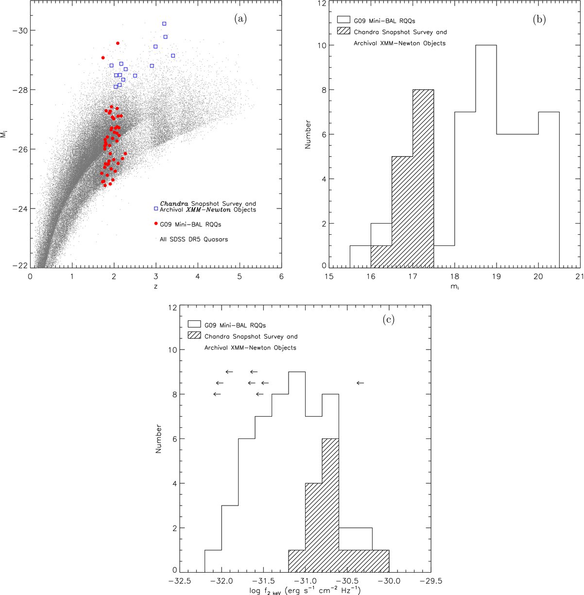
Figure 1. (a) SDSS absolute i-band magnitude, Mi, plotted with respect to redshift, z. The blue squares represent the 14 mini-BAL quasars in our combined Chandra snapshot survey and archival XMM-Newton mini-BAL quasar sample, the red circles represent the 48 mini-BAL quasars in G09, and the small black dots represent the 77,429 objects in the SDSS DR5 quasar catalog. (b) Histogram showing the distribution of SDSS i-band apparent magnitude, mi, for the objects observed in our combined Chandra snapshot survey and archival XMM-Newton mini-BAL quasar sample, relative to the 48 radio-quiet mini-BAL quasars in G09. (c) Histogram showing the distribution of X-ray flux density at rest-frame 2 keV for the objects observed in our combined Chandra snapshot survey and archival XMM-Newton mini-BAL quasar sample, relative to the 48 radio-quiet mini-BAL quasars in G09. Leftward arrows show undetected G09 sources, with arbitrary y-coordinates.
Download figure:
Standard image High-resolution imageUnless otherwise specified, a cosmology with H0 = 70 km s−1 Mpc−1, ΩM = 0.3, and ΩΛ = 0.7 will be assumed. Furthermore, the term "HiBAL" refers to BAL quasars with high-ionization states only (e.g., C iv), while "LoBAL" refers to BAL quasars with low-ionization states (e.g., Al iii or Mg ii) and usually also high-ionization states (e.g., Gibson et al. 2009b). We define positive velocities for material flowing outward with respect to the quasar emission rest frame. Section 2 discusses our sample selection, Section 3 details our X-ray data reduction and analysis, and Section 4 discusses the implications of our results. Section 5 is a summary of our conclusions.
2. SAMPLE SELECTION
We sorted the SDSS DR5 quasar catalog (Schneider et al. 2007), which covers ≈5740 deg2, by mi and identified all of the mini-BAL quasars with mi⩽ 17.5 and z ⩾ 1.9, which resulted in a list of 29 robustly identified quasars whose mini-BAL nature (as described further below) is insensitive to reasonable continuum placement. The redshift requirement ensures that all objects considered have high-quality C iv coverage in their SDSS spectra. The magnitude limit was chosen to provide a sample size that could be observed with a practical amount of Chandra observation time. The SDSS quasar catalog BEST photometric apparent i-band magnitudes were used wherever possible, but if the BEST mi = 0, then the TARGET value of mi was used. Also, we sought radio-quiet objects that were not detected by the FIRST survey (Becker et al. 1995). "Radio-quiet" is commonly defined as R < 10, where R is calculated by Equation (5) in Section 3. We required our potential targets to be covered, but undetected by the FIRST survey to minimize any X-ray emission contribution from possible jets associated with the quasars. Six of the 29 objects had FIRST detections and were therefore excluded. Furthermore, two of the radio-quiet mini-BAL quasars on our list already had X-ray coverage; we included these archival objects in our sample but did not propose new targeted Chandra observations for them. We proposed short "snapshot" (4–6 ks) Chandra observations of the resulting 21 mini-BAL quasars, generally prioritizing the targets by their brightness (mi). We were awarded observing time in Cycle 10 for 12 of the brightest objects on the target list.
Our resulting sample thus consists of 14 of the optically brightest mini-BAL quasars in the SDSS DR5 quasar catalog, as shown in Figure 1 (12 new Chandra observations and two archival XMM-Newton observations). The XMM-Newton data for SDSS J142656.17+602550.8, also known as SBS 1425 + 606, were previously published in Shemmer et al. (2008). Relevant X-ray information for SDSS J160222.72+084538.4, observed by XMM-Newton at 17 0 off-axis, is located in the XMM-Newton Serendipitous Source Catalog (2XMMi; Watson et al. 2009). For both of the XMM-Newton observations, only data from the pn detector were used, because of its high sensitivity and number of counts with respect to the MOS detectors. An observing log is shown in Table 1. Compared to the mini-BAL quasar sample (48 objects, all of which have X-ray coverage) utilized in G09, nearly all of the objects in our sample are brighter in both apparent i-band magnitude, mi, and absolute i-band magnitude, Mi. There are, however, two objects from G09 in Figure 1(b) that are comparably bright in mi to our sample objects. One is the well-known gravitationally lensed quasar PG 1115+080 (e.g., Michalitsianos et al. 1996; Chartas et al. 2007). This object was not included in our sample because its redshift of 1.74 does not meet our z ⩾ 1.9 criterion. The other object, SDSS J231324.45+003444.5, likely has a high-velocity C iv BAL in its spectrum, but was included in the sample from G09 as an "ambiguous" mini-BAL source. See Section 2.1 in G09 for a more detailed discussion regarding this source.
Table 1. Observation Log
| Object Name (SDSS J) | z | Observation | Exposure Time |
|---|---|---|---|
| Date | (ks)a | ||
| Chandra cycle 10 objects | |||
| 080117.79+521034.5 | 3.23 | 2009 Jan 12 | 4.1 |
| 091342.48+372603.3 | 2.13 | 2009 Jan 22 | 5.1 |
| 092914.49+282529.1 | 3.41 | 2009 Jan 7 | 5.0 |
| 093207.46+365745.5 | 2.90 | 2009 Jan 9 | 5.5 |
| 105158.74+401736.7 | 2.17 | 2009 Jan 20 | 4.1 |
| 105904.68+121024.0 | 2.50 | 2009 Feb 1 | 4.1 |
| 120331.29+152254.7 | 2.99 | 2009 Mar 14 | 4.1 |
| 123011.84+401442.9 | 2.05 | 2009 Oct 12 | 5.0 |
| 125230.84+142609.2 | 1.94 | 2009 Feb 28 | 4.0 |
| 141028.14+135950.2 | 2.22 | 2009 Nov 28 | 4.1 |
| 151451.77+311654.0 | 2.14 | 2008 Dec 6 | 4.1 |
| 224649.29−004954.3 | 2.04 | 2009 Jan 2 | 5.1 |
| Archival XMM-Newton objects | |||
| 142656.17+602550.8b | 3.20 | 2006 Nov 12 | 7.0 |
| 160222.72+084538.4 | 2.28 | 2003 Aug 9 | 13.3 |
Notes. aThe Chandra and XMM-Newton exposure times are corrected for detector dead time. bThe data for SDSS J142656.17+602550.8 were originally published in Shemmer et al. (2008), and it is also known as SBS 1425+606. The exposure time used here is the pn detector exposure listed in Table 1 of Shemmer et al. (2008); exposure times for the MOS1 and the MOS2 detectors were 20.6 ks and 20.9 ks, respectively.
Download table as: ASCIITypeset image
The two quantities that were used in distinguishing mini-BALs from BALs and non-BMBs are the extended balnicity index (BI0) and the AI. BI0 is defined as

where f(v) is the ratio of the observed spectrum to the continuum model for the spectrum as a function of velocity. The continuum model fit to the SDSS spectra was determined using the algorithm described in Section 2.1 of Gibson et al. (2008b). C is a parameter used to indicate BAL absorption. C = 1 if the spectrum is at least 10% below the continuum model for velocity widths of at least 2000 km s−1; C = 0 otherwise. The integration limits here are the same as in G09, which differ from those used in Weymann et al. (1991), but allow characterization of BALs even at low outflow velocities.
AI is defined as

where C' = 1 when the velocity width is at least 1000 km s−1 and the absorption trough falls at least 10% below the continuum; C' = 0 otherwise. The integration limits for AI are chosen such that the range of C iv outflow velocities is maximized and does not include the Si iv λ1400 emission line (Trump et al. 2006). BALs have AI>0 and BI0 > 0; mini-BALs have AI>0 and BI0 = 0; and non-BMBs have AI = 0 and BI0 = 0. Thus, the objects in our sample were selected such that, for C iv λ1549, BI0 = 0 and AI>0. All measurements of BI0, AI, and other absorption parameters are made in the rest frame of the quasar as defined by the improved redshift measurement of Hewett & Wild (2010). One mini-BAL quasar in G09, SDSS J142301.08+533311.8, is classified as a non-BMB quasar using this improved redshift value because its only broad absorption trough lies above the velocity integration limit of 29, 000 km s−1 in the AI definition.
The SDSS spectra for our sample are shown in Figure 2. These spectra are corrected for Galactic extinction according to Cardelli et al. (1989) and for fiber light loss. The light-loss correction was calculated as the average difference between the synthetic and photometric g, r, and i magnitudes for each quasar, as described in Section 3 of Just et al. (2007). The synthetic magnitudes are provided by the SDSS data pipeline and correspond to the integrated flux over the g, r, and i bandpasses in the SDSS spectrum. It is assumed that there is no variation in the flux between the SDSS photometric and spectroscopic epochs.

Figure 2. SDSS spectra for our Chandra snapshot survey sample, as well as the included archival XMM-Newton mini-BAL quasar observations, plotted with respect to rest-frame wavelength in Angstroms, using the improved redshift measurements in Hewett & Wild (2010). The region(s) contributing to the AI for the C iv λ1549 mini-BAL are marked by horizontal lines over the relevant trough(s). The y-coordinates of these horizontal lines are arbitrary. On each spectrum, the C iv rest wavelength is marked by a dashed line at 1550.77 Å; the maximum outflow velocity, vmax, is marked by a dotted line; and the minimum outflow velocity, vmin, is marked by a dot-dashed line. Each panel is labeled with the SDSS object name, AI, and redshift. The left column corresponds to quasars at 1.9 ⩽z< 2.5, and the right column corresponds to quasars at 2.5 ⩽z< 3.5. Dividing the sources into two columns is only for presentation purposes. Each spectrum is corrected for Galactic extinction, according to Cardelli et al. (1989), and for fiber light loss, according to the procedure outlined in Section 2. The spectral resolution (λ/Δλ) is ≈ 2000.
Download figure:
Standard image High-resolution imageThe rest wavelength of C iv λ1549 is indicated in Figure 2, as well as the minimum (vmin) and maximum (vmax) outflow velocities. The wavelengths of absorption troughs can be converted to outflow velocities using the Doppler effect formulae. vmax (vmin) is the outflow velocity corresponding to the shortest (longest) wavelength associated with the C iv λ1549 mini-BAL troughs. For quasars with a single absorption trough, vmax and vmin mark the boundaries of the absorption trough where the C' parameter in Equation (2) equals unity. To keep consistency with previous works on BAL and mini-BAL quasars (e.g., Trump et al. 2006; G09; Gibson et al. 2009b), the rest wavelength used for C iv λ1549 is 1550.77 Å, which is the red component of the C iv doublet line (Verner et al. 1996). Relevant properties of the C iv mini-BALs are shown in Table 2.
Table 2. C iv Mini-BAL Properties
| Object Name (SDSS J) | AI | vmin | vmax | vwta | No. of Troughs | Notesb |
|---|---|---|---|---|---|---|
| (km s−1) | (km s−1) | (km s−1) | (km s−1) | Contributing to AI | ||
| Chandra cycle 10 objects | ||||||
| 080117.79+521034.5 | 251.0 | 26036 | 27132 | 26641 | 1 | |
| 091342.48+372603.3 | 625.8 | 10767 | 23014 | 14463 | 2 | Feature at ≈1535 Å fails width criterion |
| 092914.49+282529.1 | 332.2 | 23881 | 25047 | 24483 | 1 | |
| 093207.46+365745.5 | 533.6 | 3146 | 4596 | 3871 | 1 | Features at ≈1480 Å and ≈1510 Å |
| fail width and depth criteria | ||||||
| 105158.74+401736.7 | 239.3 | 1805 | 2910 | 2383 | 1 | |
| 105904.68+121024.0 | 2384.7 | 5378 | 23349 | 11445 | 5 | |
| 120331.29+152254.7 | 311.3 | 21530 | 22629 | 22118 | 1 | |
| 123011.84+401442.9 | 556.8 | 1710 | 2953 | 2326 | 1 | |
| 125230.84+142609.2 | 528.7 | 2165 | 3615 | 2914 | 1 | Features at ≈1440 Å and ≈1520 Å |
| fail depth and width criteria | ||||||
| 141028.14+135950.2 | 191.6 | 1842 | 2946 | 2394 | 1 | |
| 151451.77+311654.0 | 456.0 | 25290 | 27003 | 26188 | 1 | Feature at ≈1430 Å fails both depth and |
| width criteria | ||||||
| 224649.29−004954.3 | 668.5 | 4199 | 5648 | 4858 | 1 | |
| Archival XMM-Newton objects | ||||||
| 142656.17+602550.8 | 356.0 | 27229 | 28324 | 27811 | 1 | Feature at ≈1525 Å fails width criterion |
| 160222.72+084538.4 | 316.4 | 14068 | 15239 | 14689 | 1 | Feature at ≈1540 Å fails width criterion |
Notes. aThe weighted average velocity of mini-BAL troughs. See specific definition in Section 4.4. bThis column contains explanations as to why some non-negligible absorption troughs seen in Figure 2 were not included in the AI. A trough is excluded from AI if it fails the width criterion and/or the depth criterion. The "width criterion" requires that the trough has a velocity width between 1000 and 2000 km s−1. The "depth criterion" requires that the trough remains at least 10% below the continuum. The depth criterion can be failed if there is a peak inside the absorption trough that rises above this level.
Download table as: ASCIITypeset image
3. X-RAY DATA ANALYSIS
Source detections were performed with the wavdetect algorithm (Freeman et al. 2002) using a detection threshold of 10−4 and wavelet scales of 1,  , 2,
, 2,  , and 4 pixels; all 12 Chandra targets were detected within 0
 6 of the object's SDSS coordinates. Aperture photometry was performed for each object using IDL aper routine with an aperture radius of 3'' and inner and outer annulus radii of 6'' and 9'' for background subtraction, respectively. The resulting counts in the observed-frame soft (0.5–2.0 keV), hard (2.0–8.0 keV), and full (0.5–8.0 keV) X-ray bands are reported in Table 3. Errors on the X-ray counts were calculated using Poisson statistics corresponding to the 1σ significance level according to Tables 1 and 2 of Gehrels (1986). The band ratios and the effective power-law photon indices are also included in Table 3. The band ratio is defined as the number of hard-band counts divided by the number of soft-band counts. The errors on the band ratio correspond to the 1σ significance level and were calculated using Equation (1.31) in Section 1.7.3 of Lyons (1991). The band ratios for all of the Chandra objects can be directly compared with one another because they were all observed during the same cycle. The effective power-law photon index is the photon index of the presumed Galactic-absorbed power-law spectral model for each source, under which the band ratio would be the value calculated from the X-ray counts. It was calculated using the Chandra PIMMS 5 tool (version 3.9k), using the Chandra Cycle 10 instrument response to account for the decrease in instrument efficiency over time.
Table 3. X-ray Counts
| Object Name (SDSS J) | Full Band | Soft Band | Hard Band | Band | Γ |
|---|---|---|---|---|---|
| (0.5–8.0 keV) | (0.5–2.0 keV) | (2.0–8.0 keV) | Ratio | ||
| Chandra cycle 10 objects | |||||
| 080117.79+521034.5 | 23.9+6.0−4.9 | 20.2+5.6−4.4 | 3.8+3.1−1.9 | 0.19+0.16−0.10 | 2.3+0.7−0.6 |
| 091342.48+372603.3 | 63.8+9.0−8.0 | 38.8+7.3−6.2 | 25.0+6.1−5.0 | 0.64+0.20−0.16 | 1.1+0.3−0.2 |
| 092914.49+282529.1 | 33.0+6.8−5.7 | 30.0+6.5−5.4 | 3.0+2.9−1.6 | 0.10+0.10−0.06 | 2.8+0.7−0.6 |
| 093207.46+365745.5 | 59.5+8.8−7.7 | 53.8+8.4−7.3 | 5.7+3.5−2.3 | 0.11+0.07−0.05 | 2.7+0.5−0.4 |
| 105158.74+401736.7 | 209.8+15.5−14.5 | 168.2+14.0−13.0 | 41.6+7.5−6.4 | 0.25+0.05−0.04 | 2.0+0.2−0.2 |
| 105904.68+121024.0 | 44.6+7.7−6.7 | 34.8+7.0−5.9 | 9.8+4.2−3.1 | 0.28+0.13−0.10 | 1.9+0.4−0.4 |
| 120331.29+152254.7 | 94.5+10.8−9.7 | 76.6+9.8−8.7 | 17.9+5.3−4.2 | 0.23+0.08−0.06 | 2.0+0.3−0.3 |
| 123011.84+401442.9 | 81.7+10.1−9.0 | 60.8+8.8−7.7 | 20.9+5.6−4.5 | 0.34+0.11−0.09 | 1.7+0.3−0.2 |
| 125230.84+142609.2 | 53.0+8.3−7.3 | 40.0+7.4−6.3 | 13.0+4.7−3.5 | 0.32+0.13−0.10 | 1.7+0.3−0.3 |
| 141028.14+135950.2 | 65.3+9.1−8.1 | 50.8+8.2−7.1 | 14.9+5.0−3.8 | 0.29+0.11−0.09 | 1.8+0.3−0.3 |
| 151451.77+311654.0 | 22.6+5.8−4.7 | 19.8+5.5−4.4 | 2.8+2.9−1.6 | 0.14+0.15−0.08 | 2.5+0.8−0.7 |
| 224649.29−004954.3 | 75.4+9.7−8.7 | 58.0+8.7−7.6 | 17.4+5.3−4.1 | 0.30+0.10−0.08 | 1.9+0.3−0.3 |
| Archival XMM-Newton objects | |||||
| 142656.17+602550.8 | 237.0+16.4−15.4 | 167.0+14.0−12.9 | 53.0+8.3−7.3 | 0.32+0.06−0.05 | 1.8+0.1−0.1 |
| 160222.72+084538.4a | 16.0+5.1−4.0 | 13.4+4.8−3.6 | 2.6+2.8−1.5 | ⋅⋅⋅ | ⋅⋅⋅ |
Note. aThe counts for SDSS J160222.72+084538.4 are converted from the counts in the 2XMM catalog, using an absorbed power-law model with Γ = 2 and the Galactic NH in Column 5 of Table 4.
Download table as: ASCIITypeset image
The key X-ray, optical, and radio properties of our sample are listed in Table 4.
Table 4. X-ray, Optical, and Radio Properties
| Count | log L | log Lν | |||||||||||
|---|---|---|---|---|---|---|---|---|---|---|---|---|---|
| Object Name (SDSS J) | z | mia | Mi | NH | Rateb | F0.5–2 keVc | f2 keVd | (2–10 keV) | f2500 Åe | (2500 Å) | αox | Δαox (σ)f | R |
| (1) | (2) | (3) | (4) | (5) | (6) | (7) | (8) | (9) | (10) | (11) | (12) | (13) | (14) |
| Chandra cycle 10 objects | |||||||||||||
| 080117.79+521034.5 | 3.23 | 16.76 | -29.78 | 4.58 | 4.92+1.35−1.09 | 1.99 | 12.52 | 45.33 | 8.17 | 32.25 | −1.85 | −0.04 (0.29) | <0.51 |
| 091342.48+372603.3 | 2.13 | 17.38 | −28.16 | 1.91 | 7.67+1.44−1.23 | 2.87 | 13.40 | 45.05 | 3.60 | 31.59 | −1.70 | 0.02 (0.12) | <0.73 |
| 092914.49+282529.1 | 3.41 | 17.45 | −29.14 | 2.06 | 6.02+1.31−1.09 | 2.26 | 14.84 | 45.44 | 4.28 | 32.01 | −1.71 | 0.07 (0.49) | <0.74 |
| 093207.46+365745.5 | 2.90 | 17.42 | −28.80 | 1.37 | 9.85+1.54−1.34 | 3.63 | 21.10 | 45.48 | 3.98 | 31.86 | −1.64 | 0.11 (0.78) | <1.24 |
| 105158.74+401736.7 | 2.17 | 16.71 | −28.87 | 1.33 | 41.22+3.43−3.17 | 15.16 | 71.67 | 45.79 | 6.75 | 31.88 | −1.53 | 0.23 (1.60) | <0.31 |
| 105904.68+121024.0 | 2.50 | 17.43 | −28.47 | 2.11 | 8.45+1.69−1.42 | 3.18 | 16.62 | 45.27 | 3.96 | 31.75 | −1.68 | 0.06 (0.41) | <0.68 |
| 120331.29+152254.7 | 2.99 | 16.87 | −29.45 | 3.03 | 18.82+2.41−2.15 | 7.27 | 43.09 | 45.81 | 7.28 | 32.14 | −1.62 | 0.17 (1.31) | <0.57 |
| 123011.84+401442.9 | 2.05 | 16.97 | −28.48 | 1.66 | 12.09+1.76−1.55 | 4.50 | 20.44 | 45.21 | 5.11 | 31.71 | −1.69 | 0.05 (0.32) | <0.54 |
| 125230.84+142609.2 | 1.94 | 16.55 | −28.81 | 2.13 | 10.05+1.86−1.58 | 3.80 | 16.69 | 45.07 | 7.37 | 31.83 | −1.78 | −0.03 (0.22) | <0.49 |
| 141028.14+135950.2 | 2.22 | 17.30 | −28.34 | 1.39 | 12.41+2.00−1.74 | 4.57 | 21.89 | 45.29 | 4.21 | 31.68 | −1.64 | 0.09 (0.59) | <0.79 |
| 151451.77+311654.0 | 2.14 | 17.06 | −28.49 | 1.84 | 4.78+1.34−1.07 | 1.79 | 8.33 | 44.84 | 4.88 | 31.72 | −1.83 | −0.09 (0.64) | <0.26 |
| 224649.29−004954.3 | 2.04 | 17.47 | −28.10 | 5.13 | 11.37+1.70−1.49 | 4.67 | 21.18 | 45.22 | 3.59 | 31.55 | −1.62 | 0.09 (0.61) | <1.28 |
| Archival XMM-Newton objects | |||||||||||||
| 142656.17+602550.8 | 3.20 | 16.21 | −30.22 | 1.75 | 23.86+1.99−1.84 | 6.02 | 37.72 | 45.80 | 12.48 | 32.43 | −1.82 | 0.02 (0.12) | <0.50 |
| 160222.72+084538.4 | 2.28 | 17.05 | −28.69 | 3.71 | 11.68+1.92−1.66g | 3.18 | 15.48 | 45.16 | 5.58 | 31.83 | −1.75 | 0.00 (0.02) | <0.99 |
Notes. aThe apparent i-band magnitude using the SDSS quasar catalog BEST photometry. bThe count rate in the observed-frame soft X-ray band (0.5–2.0 keV) in units of 10−3 s−1. cThe Galactic absorption-corrected observed-frame flux between 0.5and2.0 keV in units of 10−14 erg cm−2 s−1. dThe flux density at rest-frame 2 keV, in units of 10−32 erg cm−2 s−1 Hz−1. eThe flux density at rest-frame 2500 Å in units of 10−27 erg cm−2 s−1 Hz−1. fΔαox: the difference between the measured αox and the expected αox, defined by the αox − L2500 Å relation in Equation (3) of Just et al. (2007); the statistical significance of this difference, σ, is measured in units of the rms αox defined in Table 5 of Steffen et al. (2006). gCalculated using an effective exposure time corrected for vignetting at large off-axis angle.
Download table as: ASCIITypeset image
Column 1: the SDSS J2000 equatorial coordinates for the quasar.
Column 2: the quasar's redshift. These values were taken from the improved measurements in Hewett & Wild (2010), which have significantly reduced systematic biases compared to the redshift values in the SDSS DR5 quasar catalog.
Column 3: the apparent i-band magnitude of the quasar using the SDSS quasar catalog BEST photometry, mi.
Column 4: the absolute i-band magnitude for the quasar, Mi, from the SDSS DR5 quasar catalog, which was calculated assuming a power-law continuum index of αν = −0.5.
Column 5: the Galactic neutral hydrogen column density obtained with the Chandra COLDEN tool, in units of 1020 cm−2.
Column 6: the count rate in the observed-frame soft X-ray band (0.5–2.0 keV), in units of 10−3 s−1.
Column 7: the Galactic extinction-corrected flux in the observed-frame soft X-ray band (0.5–2.0 keV) obtained with PIMMS, in units of 10−14 erg cm−2 s−1. An absorbed power-law model was used with a photon index Γ = 2, which is typical for quasars and is consistent with joint X-ray spectral fitting (see Section 4.1). The Galactic neutral hydrogen column density was used for each quasar (NH, given in Column 5 of Table 4).
Column 8: the flux density at rest-frame 2 keV obtained with PIMMS, in units of 10−32 erg cm−2 s−1 Hz−1. Our sources are generally brighter in 2 keV X-ray flux density than the mini-BAL quasars in G09 (see Figure 1(c)).
Column 9: the logarithm of the Galactic extinction-corrected quasar luminosity in the rest-frame 2–10 keV band obtained with PIMMS.
Columns 10 and 11: the flux density at rest-frame 2500 Å in units of 10−27 erg cm−2 s−1 Hz−1 and the logarithm of the monochromatic luminosity at rest-frame 2500 Å, respectively. The flux density was obtained using a method similar to that described in Section 2.2 of Vignali et al. (2003). It is calculated as an interpolation between the fluxes of two SDSS filters bracketing rest-frame 2500 Å. A bandpass correction is applied when converting flux into monochromatic luminosity.
Column 12: the X-ray-to-optical power-law slope, given by

The value of αox for SDSS J142656.17+602550.8 was taken directly from Shemmer et al. (2008).
Column 13: Δαox, defined as

The expected value of αox for a typical quasar is calculated from the established αox − L2500 Å correlation given as Equation (3) of Just et al. (2007). The statistical significance of this difference, given in parentheses, is in units of σ, where σ is given in Table 5 of Steffen et al. (2006) as the rms αox for various luminosity ranges. Here, σ = 0.146 for 31 < logL2500 Å < 32 and σ = 0.131 for 32 < logL2500 Å < 33.
Column 14: the radio-loudness parameter, given by

The denominator, f4400 Å, was found via extrapolation from f2500 Å using an optical/UV power-law slope of αν = −0.5. The numerator, f5 GHz, was found using a radio power-law slope of αν = −0.8 and a flux at 20 cm, f20 cm, of three times the rms noise in a 05 × 05 FIRST image cutout at the object's coordinates. All the quantities of flux density here are per unit frequency. This value of f20 cm was used as an upper limit because there were no FIRST detections. R is thus listed as an upper limit for all of the objects. All the upper limits are well below the commonly used criterion for radio-quiet objects (R < 10). Therefore any X-ray emission from jets can be neglected.
4. DISCUSSION
4.1. Joint X-ray Spectral Analysis
Constraining X-ray spectral properties, especially the power-law photon index and the intrinsic absorption column density, can shed light on the X-ray generation mechanisms and the nuclear environments of mini-BAL quasars. We investigate the X-ray spectra of the 12 mini-BAL quasars observed in the Chandra snapshot survey. Joint spectral fitting is performed for the 12 sources, most of which do not have sufficient counts for individual analysis. We only did spectral fitting individually for one source (SDSS J1051+4017) which has ≈210 counts. Excluding this source in the joint fitting does not significantly change the best-fit parameters, which indicates that this source does not introduce biases into the joint fitting. The X-ray spectra were extracted with the CIAO routine psextract using an aperture of 3'' radius centered on the X-ray position for each source. Background spectra were extracted using an annulus with an inner radius of 6'' and outer radius of 9''. All background regions are free of X-ray sources.
Spectral analysis was carried out with XSPEC version 12.5.1 (Arnaud 1996) using the C-statistic (Cash 1979). The X-ray spectrum for each source was grouped to have at least one count per energy bin. This grouping procedure avoided zero-count bins while allowing retention of all spectral information. The C-statistic is well suited to the low-count scenario of our analysis (e.g., Nousek & Shue 1989). Each source is assigned its own redshift and Galactic column density in the joint fitting. The following models were employed in the spectral fitting: (1) a power-law model with a Galactic absorption component represented by the wabs model in XSPEC (Morrison & McCammon 1983), in which the Galactic column density is fixed to the values from COLDEN (see Column 5 in Table 4); (2) a model similar to the first, but adding an intrinsic (redshifted) neutral absorption component, represented by the zwabs model. The errors or the upper limits for the best-fit spectral parameters are quoted at 90% confidence level for one parameter of interest (ΔC = 2.71; Avni 1976; Cash 1979).
Table 5 shows the X-ray spectral fitting results. For the individually fitted source, SDSS J1051+4017, the best-fit photon index is Γ = 1.99+0.21−0.21 without adding intrinsic absorption. This value is consistent with that from band-ratio analysis (see Table 3). After adding the intrinsic absorption component, the photon index changes insignificantly to Γ = 2.06+0.37−0.26. The power-law becomes slightly steeper. The constraint on the intrinsic column density is weak (NH ≲ 1.8 × 1022 cm−2). The spectrum of this source is shown in Figure 3(a), binned to have at least 10 counts per bin for the purpose of presentation. For the joint fitting, the mean photon index is Γ = 1.90+0.11−0.11 in the model without intrinsic absorption. After adding the intrinsic absorption component, the mean photon index changes slightly to Γ = 1.91+0.14−0.11. This result is consistent with the absence of evidence for strong intrinsic neutral absorption on average (NH ≲ 8.2 × 1021 cm−2). An F-test shows that adding an intrinsic absorption component does not significantly improve the fit quality (ΔC = 0.15 for SDSS J1051+4017; ΔC = 0.01 for the joint fitting). The XMM-Newton archival source, SDSS J1426+6025, has similar X-ray spectral properties (Γ = 1.76+0.14−0.13, NH ≲ 2.3 × 1022 cm−2; Shemmer et al. 2008). The lack of substantial intrinsic absorption in these mini-BAL quasar spectra shows that mini-BAL quasars are more similar to non-BMB quasars in their X-ray absorption properties. Figure 3(b) shows a contour plot of the Γ–NH parameter space for the joint fitting with intrinsic absorption added.

Figure 3. (a) X-ray spectrum of SDSS J1051+4017 (binned to at least 10 counts per bin for the purpose of presentation) fitted with the power-law model with both Galactic and intrinsic absorption. The residuals are shown in units of σ. (b) The contour map of the photon index vs. intrinsic column density at confidence levels of 68%, 90%, and 99%, for the joint fitting of 12 Chandra snapshot survey sources.
Download figure:
Standard image High-resolution imageTable 5. X-ray Spectral Analysis
| Sources | Counts | Power Law | Power Law | |||
|---|---|---|---|---|---|---|
| Total Full-band | with Galactic Absorption | with Galactic and Intrinsic Absorption | ||||
| Γ | C-Statistic (binsa) | Γ | NH(1022 cm−2) | C-Statistic (binsa) | ||
| SDSS J105158.74+401736.7 | 210 | 1.99+0.21−0.21 | 106.17(111) | 2.06+0.37−0.26 | <1.77 | 106.02(111) |
| All 12 Chandra snapshot survey objects | 815 | 1.90+0.11−0.11 | 523.18(599) | 1.91+0.14−0.11 | <0.82 | 523.17(599) |
Note. aThe number of bins is smaller than the number of total counts because of the grouping of the spectra (see Section 4.1).
Download table as: ASCIITypeset image
We also investigated whether an ionized intrinsic absorber could better describe the X-ray spectra of the mini-BAL quasars. The absori model (Done et al. 1992), instead of the previously used zwabs model, was used to represent intrinsic absorption. The absori model has more spectral parameters and thus requires higher-quality X-ray spectra for the placement of useful spectral constraints. However, due to the limited counts of the sources in our sample, the X-ray spectral fitting could not provide a preference between the neutral and ionized intrinsic absorption models.
4.2. Relative X-ray Brightness
The Δαox parameter, defined by Equation (4), quantifies the relative X-ray brightness of a mini-BAL quasar with respect to a typical non-BMB quasar with the same UV luminosity. Figures 4 and 5 show the distributions of αox and Δαox, respectively, for our sample, as well as the non-BMB, mini-BAL and HiBAL quasars in G09. The mean values of αox and Δαox were calculated using the Kaplan–Meier estimator implemented in the Astronomy Survival Analysis (ASURV) package (e.g., Lavalley et al. 1992). A filled triangle with horizontal error bars is used to show the mean value of αox and Δαox for our sample combined with the G09 mini-BAL quasars. The mean values for αox and Δαox for the non-BMB and HiBAL quasars in the G09 sample only are shown using a filled square with horizontal error bars.

Figure 4. Top panel: histogram showing the distribution of αox for the radio-quiet non-BMB quasars in G09. Upper limits corresponding to 1σ for the non-detections are indicated by arrows, where the y-coordinates of these arrows are arbitrary. The mean value of αox, described in Section 4.2, for the radio-quiet non-BMB quasars in G09 is shown by a filled square and its horizontal error bars. The y-coordinate of the mean-value point is arbitrary, and the error bars are so small that they are only slightly visible on the plot. Middle panel: histogram showing the distribution of αox for the objects observed in our Chandra snapshot survey and archival XMM-Newton mini-BAL quasar sample, relative to the 48 radio-quiet mini-BAL quasars from G09. Upper limits corresponding to 1σ for the non-detected mini-BAL quasars in G09 are indicated by arrows. The mean value of αox for our mini-BAL quasar sample, combined with the mini-BAL quasars in G09, is shown by a filled triangle and its horizontal error bars. Bottom panel: histogram showing the distribution of αox for the radio-quiet HiBAL quasars presented in G09. Upper limits corresponding to 1σ for non-detections are indicated by arrows. The mean value of αox for the HiBAL quasars in G09 is shown by a filled square and its horizontal error bars.
Download figure:
Standard image High-resolution image
Figure 5. Top panel: histogram showing the distribution of Δαox for the radio-quiet non-BMB quasars in G09. Upper limits corresponding to 1σ for non-detections are indicated by arrows, where the y-coordinates of these arrows are arbitrary. The mean value of Δαox, described in Section 4.2, for the non-BMB quasars in G09 is shown by a filled square and its horizontal error bars. The y-coordinate of the mean-value point is arbitrary, and the error bars are so small that they are only slightly visible on the plot. Middle panel: histogram showing the distribution of Δαox for the objects observed in our combined Chandra snapshot survey and archival XMM-Newton mini-BAL quasar sample, relative to the 48 radio-quiet mini-BAL quasars from G09. Upper limits corresponding to 1σ for the non-detected mini-BAL quasars in G09 are indicated by arrows. The mean value of Δαox for our mini-BAL quasar sample, combined with the mini-BAL quasars in G09, is shown by a filled triangle and its horizontal error bars. Bottom panel: histogram showing the distribution of Δαox for the radio-quiet HiBAL quasars presented in G09. Upper limits corresponding to 1σ for non-detections are indicated by arrows. The mean value of Δαox for the HiBAL quasars in G09 is shown by a filled square and its horizontal error bars. In all three panels, the dashed line indicates Δαox = 0.
Download figure:
Standard image High-resolution imageAfter our sample is combined with the mini-BAL quasars in G09, the mean αox value, −1.68 ± 0.02, remains the same (with a smaller error bar) as the value for the mini-BAL quasar sample in G09 only. The mean Δαox value became slightly less negative once our sample was included: the mean Δαox value of our sample combined with the mini-BAL quasar sample from G09 is −0.03 ± 0.02, while it was −0.05 ± 0.03 for the G09 sample. Therefore, the mean Δαox of the combined mini-BAL quasar sample is closer to that of the non-BMB quasars in G09 (0.00 ± 0.01), which strengthens the trend that mini-BAL quasars are only slightly X-ray weaker than non-BMB quasars, while BAL quasars are considerably X-ray weaker than both mini-BAL and non-BMB quasars (the mean Δαox of the BAL quasar sample in G09 is −0.22 ± 0.04).
We have performed two-sample tests to assess if the Δαox values for mini-BAL quasars follow the same distribution as those for BAL quasars or non-BMB quasars. Gehan tests (Gehan 1965), also implemented in the ASURV package, were used on the distributions of Δαox values for the combined mini-BAL quasar sample, and the non-BMB and BAL quasar samples in G09. The Δαox distributions of mini-BAL and non-BMB quasars are not found to be different at a high level of significance; the probability of the null hypothesis from the Gehan test is 19.3%. In contrast, the Δαox distributions of mini-BAL and BAL quasars clearly differ, with a null-hypothesis probability of 0.01%. Sources with upper limits on Δαox are included in the two sample tests.
We have tested the normality of the distribution of Δαox for mini-BAL quasars. Deviations from a normal distribution, such as a skew tail, may indicate a sub-population of physically special sources (e.g., extremely X-ray weak sources) in our sample. Anderson–Darling tests (e.g., Stephens 1974) were performed on the Δαox values of the mini-BAL quasars. First, we examine the distribution of the 14 sources in our sample. The Anderson–Darling test cannot reject the hypothesis that the Δαox values follow a Gaussian distribution; the rejection probability is only 0.5%. Adding the mini-BAL quasars in G09, the sample size increases to 61. However, there are eight sources having upper limits on their Δαox values. Since the Anderson–Darling test (as well as other commonly used normality tests) can only treat uncensored data, we generate a sample of 40 sources in an unbiased way with all sources detected by considering only the mini-BAL quasars observed by Chandra with an exposure longer than 2 ks. One mini-BAL quasar in G09, SDSS J113345.62+005813.4, which is undetected in a Chandra exposure of 4.3 ks, is removed from this sample because this source likely has both intervening and intrinsic X-ray absorption (Hall et al. 2006) while we are investigating intrinsic X-ray absorption only. The probability of non-normality of the Δαox values for this sample is only 3.6%. Therefore, the Δαox values of mini-BAL quasars follow the Gaussian distribution to a reasonable level of approximation. Strateva et al. (2005) reported that for their non-BMB quasar sample (with only a few percent BAL quasar contamination), a Gaussian profile could provide a reasonable fit to the distribution of the Δαox values. Gibson et al. (2008a) also found that normality of the Δαox distribution for their radio-quiet non-BMB quasar sample could not be ruled out by the Anderson–Darling test. For our sample, we find no evidence that any significant subset of sources falls outside the Gaussian regime. Thus, mini-BAL quasars are similar to non-BMB quasars with respect to the distribution of relative X-ray brightness. We also fit the Δαox distributions using the IDL gaussfit procedure (see Figure 6). For the 14 sources in our sample, the best-fit parameters are μ = 0.04 ± 0.01, σ = 0.07 ± 0.01. For the 40 mini-BAL quasars observed by Chandra with an exposure longer than 2 ks, the fitting results are μ = 0.03 ± 0.02, σ = 0.12 ± 0.02. The measurement errors for the Δαox values for most mini-BAL quasars are ≈0.03, which is much smaller than the intrinsic spread of Δαox. In fact, the square roots of the Δαox variances for the two groups of mini-BAL quasars tested above are 0.086 and 0.137, respectively, which indicates that the measurement errors have smaller influence than the spread of Δαox.

Figure 6. Normality tests of the Δαox values for mini-BAL quasars. The bold histogram and curve represent the distribution of Δαox for the 14 sources in our sample and its best-fit Gaussian. The dotted histogram and curve represent the distribution of Δαox and its best-fit Gaussian for the 31 sources observed by Chandra with an exposure time greater than 2 ks.
Download figure:
Standard image High-resolution image4.3. Mini-BAL Quasar Reddening
BAL quasars are found to be redder than non-BMB quasars (e.g., Weymann et al. 1991; Brotherton et al. 2001; Reichard et al. 2003; Trump et al. 2006; Gibson et al. 2009b), which is likely caused by increased dust reddening. Following Gibson et al. (2009b), we investigate the reddening of mini-BAL quasars by measuring the quantity Rred, defined as,

where Fν(1400 Å) and Fν(2500 Å) are the continuum flux densities at rest-frame 1400 Å and 2500 Å, respectively. These two wavelengths approximately represent the broadest available spectral coverage for most of our mini-BAL quasars. The continuum flux densities were calculated by fitting the SDSS spectra using the algorithm described in Section 2.1 of Gibson et al. (2008b).
Figure 7 shows the distribution of Rred values for the 61 mini-BAL quasars from this work and G09. The median value of Rred is 0.70. Gibson et al. (2009b) studied the Rred values of non-BMB and BAL quasars in the redshift range 1.96 ⩽ z ⩽ 2.28, and found median Rred values for non-BMB, HiBAL, and LoBAL quasars of 0.75, 0.64, and 0.30, respectively. The median Rred of mini-BAL quasars is intermediate between those of non-BMB and HiBAL quasars. We performed Kolmogorov–Smirnov tests on the distribution of Rred values for mini-BAL quasars versus those for non-BMB, HiBAL, and LoBAL quasars in the common redshift range of 1.96 ⩽ z ⩽ 2.28. The probability of the Rred values for 27 mini-BAL quasars and for 6689 non-BMB quasars coming from the same population is 0.100, while those probabilities are 0.053 and 3.05 × 10⁻⁸ for the mini-BAL quasars compared to 904 HiBAL quasars and 82 LoBAL quasars, respectively. These results cannot distinguish whether the Rred distribution for mini-BAL quasars is more similar to that for non-BMB quasars or for HiBAL quasars.

Figure 7. Distribution of the ratio Rred ≡ Fν(1400 Å)/Fν(2500 Å) for the 61 mini-BAL quasars in the combined sample. The vertical dashed line indicates the median Rred value (0.70) for mini-BAL quasars. The three filled squares show the median Rred values for non-BMB quasars (0.75), HiBAL quasars (0.64), and LoBAL quasars (0.30) in Gibson et al. (2009b), respectively.
Download figure:
Standard image High-resolution imageThe "redness" of the mini-BAL quasars may be caused by either steeper intrinsic power-law slopes or dust reddening. We calculated the relative SDSS colors Δ(u − r), Δ(g − i), and Δ(r − z), to assess curvature in the optical continuum, which can be seen as the evidence of dust reddening (e.g., Hall et al. 2006). The relative color is defined as the difference between the source color and the modal color for SDSS quasars in the corresponding redshift bin, calculated following the method in Section 5.2 of Schneider et al. (2007). For a pure power-law continuum, these three relative colors should be equal within uncertainties, while for dust-reddened objects, we would expect curvature in the continuum, specifically, Δ(u − r)>Δ(g − i)>Δ(r − z). For our mini-BAL quasar sample, the median values6 of the three relative colors are 0.086 ± 0.025, 0.074 ± 0.018, and 0.032 ± 0.015, respectively. Kolmogorov–Smirnov tests show that the probability for Δ(u − r) and Δ(r − z) following the same distribution is 7.5 × 10⁻³, while those probabilities for Δ(u − r) versus Δ(g − i) and Δ(g − i) versus Δ(r − z) are 0.35 and 0.068, respectively. Therefore, we can see a moderate trend that Δ(u − r)>Δ(g − i)>Δ(r − z), indicating mild dust reddening in mini-BAL quasar spectra.
Assuming all quasars have a similar underlying continuum shape on average, different Rred values represent different dust-reddening levels. According to an SMC-like dust extinction curve (Pei 1992), the median Rred for mini-BAL quasars corresponds to E(B − V) ≈ 0.011, which is lower than the E(B − V) values of HiBAL quasars (≈0.023) and LoBAL quasars (≈0.14) in G09. Since the relative X-ray brightness Δαox largely represents the absorption in X-ray band, we tested for correlations between Rred and Δαox for the mini-BAL quasars using the Spearman rank-order correlation analysis. This analysis returns a correlation coefficient ρ and a corresponding probability PS for the null hypothesis (no correlation). ρ = 0 indicates no correlation between the two variables tested, while ρ = ±1 means a perfect correlation. The correlation probability is 1 − PS, e.g., PS = 0.01 means a correlation probability of 99%. We find a marginal correlation between Rred and Δαox for the 61 mini-BAL quasars in the combined sample at an 86.2% probability (ρ = 0.190).
4.4. UV Absorption Versus X-ray Brightness
We define a high signal-to-noise ratio (S/N) sample of BAL and mini-BAL quasars to study correlations between Δαox and AI, vmax, vmin, Δv (≡|vmax − vmin|) (see Section 2 for the definitions of these quantities). Radio-quiet BAL and mini-BAL quasars in G09 with S/N1700 > 9, and the 14 mini-BAL quasars analyzed in this paper (which also have S/N1700 > 9), are included in the high S/N sample. S/N1700 is defined as the median of the flux divided by the noise provided by the SDSS pipeline for spectral bins between rest-frame 1650 Å and 1700 Å. Excluding low S/N sources enables the most-reliable measurements for the UV absorption parameters listed above; Gibson et al. (2009b) reported that high S/N spectra enabled more accurate identifications of broad absorption features. The values of the AI, vmax, and vmin parameters for the sources in G09 are updated according to the improved redshift measurements in Hewett & Wild (2010). There are 23 BAL quasars (four of them have upper limits on Δαox) and 33 mini-BAL quasars (two of them have upper limits on Δαox) in the high S/N sample.
Figure 8 shows the SDSS spectra for the 33 mini-BAL quasars in the high S/N sample in order of Δαox. The positions of mini-BAL troughs are shown in the figure. Some mini-BAL troughs show doublet-like features. However, for mini-BAL quasars only, no significant trends are apparent between Δαox and the positions or morphologies of mini-BAL troughs.

Figure 8. SDSS spectra for the 14 mini-BAL quasars in our sample (blue curves) and the high S/N mini-BAL quasars in G09 (black curves), in the order of Δαox. The Δαox values and their error bars (if the source is detected in X-rays) are shown for each source. The name of each source is labeled in the format of "Jhhmm" for brevity (except J095820 and J095834). The y-coordinates are arbitrary. The left threshold of the x-coordinates (1407.36 Å) corresponds to the velocity integration limit of 29, 000 km s−1 in the definition of mini-BALs. As in Figure 2, the dashed lines show the rest-frame wavelength (1550.77 Å) of C iv. For each spectrum, the black horizontal bars and the black solid vertical line show the absorption troughs and weighted average velocity vwt (see Equation (7) for definition) under the velocity width limit of 1000 km s−1, respectively. The red horizontal bars show the absorption troughs that would be included if the velocity width limit were chosen to be 500 km s−1. The red dotted vertical line shows the accordingly changed vwt. Sources with asterisks after their names are excluded in the VHS mini-BAL quasar sample as defined in Section 4.6.
Download figure:
Standard image High-resolution imageIn Figure 9, we plot the UV absorption properties against Δαox for the high S/N mini-BAL and BAL quasar sample. The correlation probabilities between Δαox and AI, vmax, vmin, Δv are determined using Spearman rank-order correlation analysis (see Table 6). Our correlations are consistent with those found in G09. Our enhanced correlation between AI and Δαox confirms the trend found in G09 that UV broad absorption strength decreases with the relative X-ray brightness. As in G09, vmax is correlated with Δαox, while there is no significant correlation between vmin and Δαox. The Δv–Δαox correlation shows that mini-BAL quasars with narrower absorption troughs are relatively X-ray brighter than BAL quasars. Some mini-BAL quasars have large Δv values because they have multiple absorption troughs.

Figure 9. (a) C iv λ1549 AI plotted with respect to Δαox for our combined Chandra snapshot survey and archival XMM-Newton radio-quiet mini-BAL quasar sample (open circles), as well as the detected radio-quiet HiBAL (filled triangles) and mini-BAL (filled squares) quasars from G09. Upper limits for the G09 undetected HiBAL quasars are indicated by arrows, while the undetected mini-BAL quasar upper limits are indicated by asterisks. All of the objects have SN1700 > 9. (b) C iv λ1549 maximum outflow velocity, vmax, plotted vs. Δαox. (c) C iv λ1549 minimum outflow velocity, vmin, plotted vs. Δαox. (d) C iv λ1549 velocity difference, Δv = |vmax − vmin| plotted vs. Δαox. (e) C iv λ1549 weighted average velocity vwt, plotted vs. Δαox. The numbers in the parentheses of the y-axis titles (1000 km s−1) are the units for corresponding quantities. The results of the Spearman rank-order correlation analyses (correlation coefficient ρ and probability 1 − PS; also listed in Table 6) are shown in each panel.
Download figure:
Standard image High-resolution imageTable 6. Spearman Rank-order Correlation Coefficients and Probabilities
| Correlation | G09 Sample | G09 Sample | G09 mini-BAL only | |||||
|---|---|---|---|---|---|---|---|---|
| G09 Samplea | + Our Sample | + Our Sample | + Our Sample | |||||
| (1000 km s−1)b | (1000 km s−1)b | (500 km s−1)b | (500 km s−1)b | |||||
| ρ | 1 − PS | ρ | 1 − PS | ρ | 1 − PS | ρ | 1 − PS | |
| AI vs. Δ αox | −0.474 | 99.76% | −0.519 | 99.99% | −0.599 | >99.99% | −0.434 | 98.59% |
| vmax vs. Δ αox | −0.442 | 99.54% | −0.380 | 99.52% | −0.409 | 99.76% | −0.402 | 97.69% |
| vmin vs. Δ αox | −0.014 | 7.00% | −0.055 | 32.74% | −0.189 | 83.92% | −0.252 | 84.56% |
| Δv vs. Δ αox | −0.620 | 99.99% | −0.628 | >99.99% | −0.463 | 99.94% | −0.422 | 98.30% |
| vwt vs. Δ αox | −0.191 | 78.99% | −0.205 | 87.24% | −0.252 | 93.85% | −0.260 | 85.87% |
Notes. aThe correlation analysis for G09 sample sources only is repeated with the Spearman rank-order correlation analysis, using updated AI, vmax, vmin, and Δv values according to the improved redshift measurements in Hewett & Wild (2010). bVelocity width limit used when defining mini-BALs.
Download table as: ASCIITypeset image
We have calculated the weighted average velocity, vwt, which is defined in Trump et al. (2006) using the following equation,

where f(v) and C' have the same definition as in Equation (2). The values of vwt for the 14 mini-BAL quasars in our sample are listed in Table 2 and also shown in Figure 8. The vwt parameter represents the weighted average position of mini-BAL and BAL troughs. However, for some mini-BAL quasars with multiple absorption troughs, vwt may fall between troughs where no absorption features are present. vwt is marginally correlated with Δαox at a probability of 87.9% for the high S/N sample of mini-BAL and BAL quasars (see Figure 9(e)).
In the disk-wind model for BAL and mini-BAL quasars (e.g., Murray et al. 1995), the UV absorbing outflow is radiatively accelerated, while the material interior to the UV absorber shields the soft X-ray radiation to prevent overionization. This model may be supported by the correlations between UV absorption properties and relative X-ray weakness (see Table 6). As in G09, we also find some high velocity, relatively X-ray bright mini-BAL quasars in our newly analyzed 14 sources. These sources can perhaps be fit into the "failed" BAL quasar scenario discussed in Section 4.2 of G09, in which the high incident X-ray flux overionizes the outflow material so that BAL troughs cannot form along the line of sight.
4.5. Alternative Measures of UV Absorption
4.5.1. Effects of the Velocity Width Limit
From the rest-frame UV spectra of mini-BAL quasars (e.g., Figure 2), we can see that some likely intrinsic absorption features are missed by the definition of mini-BALs using the parameter AI (also see the "Notes" column of Table 2). When calculating AI, only absorption troughs with velocity widths greater than 1000 km s−1 are included. This somewhat conservative velocity width limit was adopted because we wanted to spend valuable Chandra observing time only on sources with bona fide intrinsic absorption features. Here we now slightly modify the definition of AI by lowering the velocity width limit to 500 km s−1 to form a new parameter AI500. This velocity width limit is similar to the value in the original introduction of AI (450 km s−1) in Hall et al. (2002). The limit of 500 km s−1 can include more broad absorption features while still minimizing the inclusion of, e.g., complex intervening systems (see the discussion in Hall et al. 2002). The equation for calculating AI500 is the same as that of AI,

while C* here has a different definition from C' in Equation (2): C* = 1 when the velocity width is at least 500 km s−1 and the absorption trough falls at least 10% below the continuum; C* = 0 otherwise. Five of the 14 mini-BAL quasars in our sample have new absorption troughs included using this new velocity width limit (see the blue spectra in Figure 8). The AI500, as well as vmax, vmin, Δv, and vwt also changes accordingly (see Table 7).
Table 7. C iv Mini-BAL Properties for Sources with New Absorption Troughs Included under the Definition of AI500
| Object Name (SDSS J) | AI500 | vmin | vmax | vwt | No. of Troughs | Notesa |
|---|---|---|---|---|---|---|
| (km s−1) | (km s−1) | (km s−1) | (km s−1) | Contributing to AI | ||
| Chandra cycle 10 objects | ||||||
| 091342.48+372603.3 | 1136.8 | 3179 | 23014 | 10715 | 4 | Feature at ≈1535 Å included |
| Feature at ≈1480 Å included | ||||||
| 105904.68+121024.0 | 2503.5 | 5378 | 23349 | 11717 | 6 | Feature at ≈1470 Å included |
| 151451.77+311654.0 | 692.7 | 24124 | 27003 | 25592 | 2 | Feature at ≈1430 Å included |
| Archival XMM-Newton objects | ||||||
| 142656.17+602550.8 | 478.3 | 4937 | 28324 | 21746 | 2 | Feature at ≈1525 Å included |
| 160222.72+084538.4 | 517.1 | 2136 | 15239 | 10006 | 2 | Feature at ≈1540 Å included |
Note. aThis column describes the newly included absorption troughs using the velocity width limit of 500 km s−1. As discussed in the "Notes" column of Table 2, some of them failed the width criterion when the velocity width limit was taken as 1000 km s−1.
Download table as: ASCIITypeset image
New absorption troughs are also identified for some BAL and mini-BAL quasars in G09 using the AI500 definition (e.g., see Figure 8 for mini-BAL quasars). From Figure 8, we can see that more relatively X-ray weak sources (with more negative Δαox) have new absorption troughs (indicated by the red horizontal bars) included compared to relatively X-ray bright sources. We repeated the correlation analysis between Δαox and UV absorption properties for the high S/N BAL and mini-BAL quasar sample; the results are listed in Table 6. The UV absorption properties under the new definition of AI are plotted against Δαox in Figure 10. Red data points show the quantities changed under the new definition. All UV absorption parameters, except Δv, have better correlations with Δαox, while the correlation probability between Δαox and Δv is still consistent with the previous result. vmin now has a marginal correlation (83.9%) with Δαox. If we only consider mini-BAL quasars in the high S/N sample (i.e., leaving out BAL quasars), these correlations still exist, although they are somewhat weaker (see the last two columns of Table 6). However, under the velocity width limit of 1000 km s−1, the correlation between Δαox and AI disappears (1 − PS = 60.0%) for mini-BAL quasars only, while the correlation between Δαox and vmax becomes much weaker (1 − PS = 91.4%). We consider 500 km s−1 to be a better velocity width limit than the previously used value (1000 km s−1), in the sense that it can reveal somewhat clearer correlations between X-ray and UV absorption properties. Figure 8 shows that most of the newly included absorption troughs have similar profiles and velocities to those troughs with >1000 km s−1 velocity widths. A Kolmogorov–Smirnov test does not distinguish the distributions of central velocities for the troughs with >1000 km s−1 velocity widths and those with 500–1000 km s−1 velocity widths (P = 0.46). Therefore, these newly included troughs are not likely to be caused by intervening systems.

Figure 10. UV absorption properties, AI500(a), vmax(b), vmin(c), Δv(d), and vwt(e) under the velocity width limit of 500 km s−1, plotted against Δαox. The symbols follow the same definition as in Figure 9. The red symbols show the quantities that changed under the new velocity width limit. The numbers in the parentheses of the y-axis titles (1000 km s−1) are the units for corresponding quantities. The results of the Spearman rank-order correlation analyses (correlation coefficient ρ and probability 1 − PS; also listed in Table 6) are shown in each panel.
Download figure:
Standard image High-resolution image4.5.2. Investigating New UV Absorption Parameters
The Δv parameter measures the velocity span of the UV absorbing outflow for sources with a single mini-BAL or BAL trough. However, for sources with multiple absorption troughs, Δv also includes regions where no absorption features are present. We therefore define a new parameter, called "total velocity span (vtot)," for the mini-BAL and BAL quasars. vtot is defined by the following equation,

where C* is the same as that in the definition of AI500. The values of vtot for the 14 mini-BAL quasars in our sample are listed in Table 8. The vtot parameter represents the total velocity width of all absorption troughs up to 29, 000 km s−1. vtot is correlated with Δαox at a probability of >99.99% for the high S/N sample of BAL and mini-BAL quasars (see Figure 11(a)). This strong correlation also stands for mini-BAL quasars only (1 − Ps = 99.77%).

Figure 11. (a) C iv λ1549 total velocity span, vtot, plotted vs. Δαox. (b) C iv λ1549 weighted average velocity for the strongest absorption trough vwt,st, plotted vs. Δαox. (c) C iv λ1549 K parameter plotted vs. Δαox. The symbols follow the same definition as in Figure 9. A velocity width limit of 500 km s−1 is used when calculating vtot and K values in this figure. The numbers in the parentheses of the y-axis titles (1000 km s−1 or 109 km−3 s−3) are the units for corresponding quantities. The results of the Spearman rank-order correlation analyses (correlation coefficient ρ and probability 1 − PS) are shown in each panel.
Download figure:
Standard image High-resolution imageTable 8. The Values of the vtot, vwt,st, and K Parameters for the 14 Mini-BAL Quasars
| Object Name (SDSS J) | vtot | vwt,st | K |
|---|---|---|---|
| (km s−1) | (km s−1) | (109 km3 s−3) | |
| Chandra cycle 10 objects | |||
| 080117.79+521034.5 | 1095.8 | 26641 | 4331.9 |
| 091342.48+372603.3 | 4958.8 | 11695 | 592.7 |
| 092914.49+282529.1 | 1165.7 | 24483 | 4183.3 |
| 093207.46+365745.5 | 1449.4 | 3871 | 21.9 |
| 105158.74+401736.7 | 1104.4 | 2383 | 3.1 |
| 105904.68+121024.0 | 8811.7 | 6435 | 813.3 |
| 120331.29+152254.7 | 1098.5 | 22118 | 3067.5 |
| 123011.84+401442.9 | 1242.5 | 2326 | 5.9 |
| 125230.84+142609.2 | 1449.5 | 2914 | 9.4 |
| 141028.14+135950.2 | 1725.7 | 2394 | 1.6 |
| 151451.77+311654.0 | 2329.8 | 26188 | 5002.6 |
| 224649.29-004954.3 | 1449.3 | 4858 | 53.6 |
| Archival XMM-Newton objects | |||
| 142656.17+602550.8 | 1716.1 | 27811 | 4475.0 |
| 160222.72+084538.4 | 2068.1 | 14689 | 487.2 |
Download table as: ASCIITypeset image
As mentioned in Section 4.4, the weighted average velocity, vwt, may represent regions without absorption features for spectra with multiple troughs. Therefore, we also calculated the weighted average velocity for the strongest absorption trough vwt,st using the following equation similar to the definition of vwt,

where vmin,st and vmax,st are the minimum and maximum velocity for the strongest absorption trough, which has the largest AI value (denoted by AIst) among those multiple troughs. The vwt,st values for the 14 mini-BAL quasars in our sample are listed in Table 8. vwt,st has a better correlation (98.9%) with Δαox than vwt (see Figure 11(b)).
The kinetic luminosity of an AGN outflow,  , is proportional to NHv3, where
  is the mass flux of the outflow and NH is its column density (e.g., see Section 11.3 of Krolik 1999). We define another new parameter,

K is a product of absorption strength, which is denoted by the factor 1 − f(v), and v3, averaged over the velocity parameter space. It is heuristically motivated by kinetic luminosity, but it is not a proper measure of this quantity since, e.g., absorption strength is usually not proportional to NH (cf. Hamann 1998; Arav et al. 1999). For the high S/N sample, the K parameter is correlated with Δαox at a probability of 97.1% (see Figure 11(b)). The values of K for the 14 mini-BAL quasars in our sample are also listed in Table 8.
For sources with a single broad absorption trough, vtot and vwt,st have the same values as Δv and vwt, respectively. For sources with multiple troughs, vtot and vwt,st have the advantage that they represent absorption features only. Furthermore, vtot and vwt,st have better correlations with the relative X-ray brightness. Although vtot and Δv have similar high correlation probabilities with Δαox (>99.99% versus 99.94%), Figure 11(a) versus Figure 10(d) shows that the correlation between vtot and Δαox is stronger, which is also indicated by the Spearman rank-order correlation coefficients (ρ = −0.682 versus ρ = −0.463). We consider vtot and vwt,st to be more physically revealing parameters. The other newly introduced parameter K does not have a better correlation with Δαox than the simpler parameter AI does. Further investigations may find additional useful parameters which could better represent the physical properties of UV absorbing outflows.
4.6. Investigation of a Very High Significance Mini-BAL Sample
In previous discussion and in G09, BAL and mini-BAL features were identified by formal criteria (Equations (1) and (2)). These formal criteria were used to distinguish mini-BALs from both narrower (NAL) and broader (BAL) absorption features. The identification process depends, to some extent, on continuum placement, spectral smoothing, and spectral S/N. Because they are narrower and (generally) weaker absorption features, mini-BALs can be more sensitive to small changes in these factors than BALs are. Mini-BALs selected according to the criteria in Equations (1) and (2) also exhibit a wide range of absorption trough morphologies. The current work tests and expands upon the findings of G09 using spectra with absorption features that have been selected to represent robustly an intermediate class of absorption between BAL and NAL features.
As is apparent from Figure 8, some formally selected mini-BAL troughs from G09 are not as significant as others. In order to investigate whether "borderline" sources are affecting our results, we define a very high significance (VHS) mini-BAL quasar sample from the high S/N sources in Section 4.4 by requiring that the mini-BAL troughs lie at least 20% below the continua, instead of 10%. Under this stricter depth criterion and the width criterion of 500 km s−1 (see Section 4.5 for discussion on the advantages of 500 km s−1 over 1000 km s−1), 24 of the 33 mini-BAL quasars remain in the VHS sample (see sources in Figure 8 without asterisks following their names), including 13 of the 14 sources in our newly studied sample. All the spectra of the VHS sample sources were examined by eye; they all show visually compelling intermediate absorption features.
We repeated the analyses in Sections 4.2 and 4.4 on relative X-ray brightness and its correlations with UV absorption properties for the VHS sample. The mean value of Δαox is −0.01 ± 0.03, which is consistent with that for mini-BAL quasars in Section 4.2 (−0.03 ± 0.02). The correlation analyses were performed on the VHS mini-BAL quasars combined with the high S/N BAL quasars in Section 4.4. Two BAL quasars in G09 (SDSS J0939+3556 and SDSS J1205+0201) are removed here because they have AI = 0 under the 20% depth criterion. The results are listed in Table 9. These correlations for VHS mini-BAL and BAL quasars are generally consistent with those for the high S/N sample in Section 4.4 (see Table 6). In summary, the factors in selection of mini-BALs (e.g., the placement of continua) do not significantly affect the main results of our analyses.
Table 9. Spearman Rank-order Tests for Very High Significance Mini-BAL and BAL Quasar Sample
| Correlation | VHS Mini-BAL + BAL Quasars | ||
|---|---|---|---|
| (500 km s−1)a | |||
| ρ | 1 − PS | ||
| AI vs. Δ αox | −0.503 | 99.92% | |
| vmax vs. Δ αox | −0.427 | 99.54% | |
| vmin vs. Δ αox | −0.157 | 70.17% | |
| Δv vs. Δ αox | −0.610 | 99.99% | |
| vwt vs. Δ αox | −0.270 | 92.70% | |
Note. aVelocity width limit used when defining mini-BALs.
Download table as: ASCIITypeset image
5. CONCLUSIONS
We present the X-ray properties of 14 of the optically brightest mini-BAL quasars from SDSS DR5; 12 have been observed in a new Chandra snapshot survey in Cycle 10 and 2 objects have archival XMM-Newton observations. All 14 sources are detected. We study correlations between the UV absorption properties and the X-ray brightness for a sample consisting of these 14 sources, as well as the BAL and mini-BAL quasars in G09. Our main results are summarized as follows.
- 1.The mean X-ray power-law photon index of the 12 Chandra observed sources is Γ = 1.90+0.11−0.11 for a model without intrinsic absorption. Adding an intrinsic neutral absorption component only slightly changes the mean photon index to Γ = 1.91+0.18−0.11, consistent with the absence of evidence for strong intrinsic neutral absorption on average (NH ≲ 8.2 × 1021 cm−2). This indicates that mini-BAL quasars generally have similar X-ray spectral properties to non-BMB quasars.
- 2.The relative X-ray brightness, assessed with the Δαox parameter, of the mini-BAL quasars has a closer mean value and distribution to those of non-BMB quasars than to those of BAL quasars. An Anderson–Darling test finds no non-normality of the Δαox distribution of mini-BAL quasars.
- 3.The reddening, assessed with the parameter Rred, of the mini-BAL quasars is intermediate between those of non-BMB and HiBAL quasars. Relative colors show curvature in the optical spectra of mini-BAL quasars, indicating mild dust reddening.
- 4.Significant correlations are found between Δαox and AI, vmax and Δv. The weighted average velocity vwt has a marginal correlation with Δαox. These correlations may support the radiatively driven disk-wind model where X-ray absorption is important in enabling UV line-absorbing winds.
- 5.We find that more intrinsic broad absorption troughs are included if the velocity width limit in the definition of mini-BALs is lowered to 500 km s−1. The UV absorption parameters AI, vmax, vmin, Δv, and vwt have clearer correlations with the relative X-ray brightness under the new velocity width limit. We also propose three new parameters, vtot, vwt,st, and K, defined by Equations (9), (10), and (11), respectively. vtot is the total velocity span of all the UV broad absorption troughs, while vwt,st is the weighted average velocity for the strongest absorption trough. We consider vtot and vwt,st to better represent the physical properties of UV absorption features than Δv and vwt. K is similar to, but not a proper measure of, the kinetic luminosity of the absorbing outflows.
- 6.Testing shows that the complex factors in the selection of mini-BAL quasars, such as the placement of continua, do not significantly affect our main results on the relative X-ray brightness and its correlations with UV absorption properties.
Further accumulation of high-quality X-ray and UV/optical data will allow studies of even larger samples of mini-BAL and BAL quasars. The improved source statistics should enable the construction and testing of further measures of mini-BAL and BAL absorption that may provide additional insight in the exploration of the broad absorption region. Ultimately, high-resolution X-ray spectroscopy performed by future missions, such as IXO, should reveal the detailed physical and kinematic properties of the X-ray absorber. This will open a new dimension in studies of X-ray versus UV/optical absorption for quasar outflows.
We thank the anonymous referee for constructive comments. We gratefully acknowledge the financial support of NASA grant SAO SV4-74018 (G.P.G., Principal Investigator), NASA ADP grant NNX10AC99G (J.W., W.N.B., M.L.C.), NASA Chandra grant AR9-0015X (R.R.G.), and NSF grant AST07-09394 (R.R.G.). We thank Y. Q. Xue for helpful discussions.
Funding for the SDSS and SDSS-II has been provided by the Alfred P. Sloan Foundation, the Participating Institutions, the National Science Foundation, the U.S. Department of Energy, the National Aeronautics and Space Administration, the Japanese Monbukagakusho, the Max Planck Society, and the Higher Education Funding Council for England. The SDSS Web site is http://www.sdss.org/.
Footnotes
- 5
- 6
The quoted error for the median value is estimated using
 . NMAD, the normalized median absolute deviation, is a robust estimator of the spread of the sample, defined as NMAD = 1.48 × median(|x − median(x)|) (see Section 1.2 of Maronna et al. 2006). N is the sample size, which is 61 in our case.
