THE LAGRANGE EQUILIBRIUM POINTS L₄ AND L₅ IN BLACK HOLE BINARY SYSTEM

Recent advances in numerical relativity (NR) have led to an increasing interest in the astrophysical implications of black hole (BH) mergers. Of particular interest is the possibility of a distinct, luminous electromagnetic (EM) counterpart to a gravitational-wave (GW) signal (Bloom 2009). If such an EM counterpart could be identified with a LISA³ detection of a supermassive BH binary in the merging process, then the host galaxy could likely be determined. A large variety of potential EM signatures have recently been proposed, almost all of which require some significant amount of gas in the near vicinity of the merging BHs.

Gas in the form of accretion disks around single massive BHs is known to produce some of the most luminous objects in the universe. However, very little is known about the behavior of accretion disks around two BHs, particularly at late times in their inspiral evolution. In Newtonian disks, it is believed that a circumbinary accretion disk will have a central gap of much lower density, either preventing accretion altogether, or at least decreasing it significantly (Pringle 1991; Artymowicz & Lubow 1994, 1996). When including the evolution of the binary due to GW losses, the BHs may also decouple from the disk at the point when the GW inspiral time becomes shorter than the gaseous inflow time at the inner edge of the disk (Milosavljevic & Phinney 2005). This decoupling should effectively stop accretion onto the central object until the gap can be filled on an inflow timescale. However, other semianalytic calculations predict an enhancement of accretion power as the evolving binary squeezes the gas around the primary BH, leading to a rapid increase in luminosity shortly before merger (Armitage & Natarajan 2002; Chang et al. 2010).

Setting aside for the moment the question of how the gas can or cannot reach the central BH region, a number of recent papers have shown that if there is sufficient gas present, then an observable EM signal is likely. Krolik (2010) used analytic arguments to estimate a peak luminosity comparable to that of the Eddington limit, independent of the detailed mechanisms for shocking and heating the gas. Using relativistic magneto-hydrodynamic simulations in two dimensions, O'Neill et al. (2009) showed that the prompt mass loss due to GWs actually leads to a sudden decrease in luminosity following the merger, as the gas in the inner disk temporarily has too much energy and angular momentum to accrete efficiently. Full NR simulations of the final few orbits of a merging BH binary have now been carried out including the presence of EM fields in a vacuum (Palenzuela et al. 2009, 2010; Mosta et al. 2010) and also gas, treated as test particles in van Meter et al. (2010) and as an ideal fluid in Bode et al. (2010) and Farris et al. (2010). The simulations including matter all suggest that the gas can get shocked and heated to high temperatures, thus leading to bright counterparts in the event that sufficient gas is in fact present. One estimate of "sufficient" is the condition that the gas be optically thick to electron scattering, which will lead to Eddington-rate luminosities (Krolik 2010). Thus, we require κρR ≳ 1, where κ = 0.4 cm²  g⁻¹ is the opacity and ρ is the characteristic density over a length scale R ∼ 10 GM_BH/c². Then, the total mass is a modest M_gas ∼ ρR³ ≈ 5 × 10²⁶ M²₇ g, where M₇ = M_BH/(10⁷ M_☉). More gas will generally lead to longer, but not necessarily more luminous signals.

The motivation for this work is to understand potential dynamical processes that could lead to a significant amount of gas around the BHs at the time of merger. We focus on stable orbits in the circular, restricted three-body problem, i.e., a system with two massive objects orbiting each other on circular, planar Keplerian orbits, with the third body being a test particle free to move out of the plane. Gas or stars that get captured into these stable regions at large binary separation may remain trapped as the binary orbit shrinks due to radiation reaction. In this paper, we integrate the restricted three-body equations of motion in the corotating frame for a range of BH mass ratios, including the evolution of the binary with leading-order post-Newtonian (PN) GW losses. With the exception of these non-conservative corrections, all dynamics are considered at the purely Newtonian level.

We find that particles initially close to the L₄ and L₅ Lagrange points remain on stable orbits throughout the adiabatic evolution of the BH binary. This result immediately leads to a number of astrophysical predictions. If diffuse gas is captured from the surrounding medium, and irradiated by an accretion disk around either BH, it may produce strong, relatively narrow emission lines with large velocity shifts, varying on an orbital timescale. If individual stars are captured, they may eventually get tidally disrupted by one of the BHs shortly before merger, providing an enormous source of material for accretion. Stars may also get ejected from the system at late times, producing ultra-hyper-velocity stars (ultra-HVSs) moving away from the galactic center at a significant fraction of the speed of light. Clusters of stars could also get captured or form in situ at large binary separation, then get compressed adiabatically as the BH system shrinks, ultimately collapsing from gravitational instabilities. Compact objects such as neutron stars or stellar-mass BHs would not get tidally disrupted in most cases, but could still possibly be detected with LISA as perturbations to the GW signal.

While this manuscript was in preparation, a similar work by Seto & Muto (2010) was published, with some of the same conclusions. One major distinction is that they included first-order PN terms in their equations of motion, while we do not. Also, they "have not found notable qualitative differences" between L₄ and L₅, while we do. Many of our astronomical predictions are qualitatively similar, but have been derived independently.

The outline for this paper is as follows: in Section 2, we present the three-body equations of motion, including GW losses, and analyze the stability and location of the equilibrium Lagrange points. These analytic predictions are tested in Section 3 with numerical simulations of a large number of test particles. In Section 4 we explore in more detail some potential astronomical applications of these results, and in Section 5 we conclude.

We consider a three-body system wherein the larger bodies have masses M₁ and M₂ (M₁ > M₂; M ≡ M₁ + M₂) and the third object is a test particle of negligible mass m₀. We define dimensionless masses μ₁ ≡ M₁/M and μ₂ ≡ M₂/M. M₁ and M₂ move on circular, Keplerian orbits around the center of mass at the origin with semimajor axis a(t). Unless otherwise stated, we use geometrized units with G = c = 1. In the corotating frame, we define coordinates (x, y, z), with the primary BH located at (−μ₂ a, 0, 0), the secondary at (μ₁ a, 0, 0), and the center of mass at the origin (see Figure 1). The angular velocity of the system in the lab frame is n = a^−3/2. The binary is orbiting in the +ϕ direction for the standard definition of spherical coordinates. The equations of motion for the test particle may be written as

$$\begin{equation} \ddot{x} = 2n\dot{y}+n^2x +\dot{n}y- \left[\mu _1\frac{x+a\mu _2}{r_1^3}+\mu _2\frac{x-a\mu _1}{r_2^3}\right], \end{equation} \tag{ 1a }$$

$$\begin{equation} \ddot{y} = -2n\dot{x}+n^2y -\dot{n}x- \left[\frac{\mu _1}{r_1^3}+\frac{\mu _2}{r_2^3}\right]y, \end{equation} \tag{ 1b }$$

$$\begin{equation} \ddot{z} = -\left[\frac{\mu _1}{r_1^3}+\frac{\mu _2}{r_2^3}\right]z, \end{equation} \tag{ 1c }$$

$$\begin{equation} \dot{n} = \frac{96}{5}\mu _1\mu _2 n^{11/3} \,, \end{equation} \tag{ 1d }$$

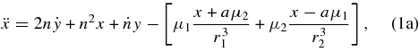
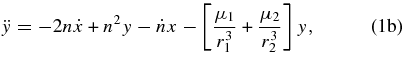
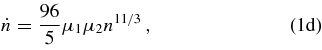
where r₁ and r₂ are the distances to the primary and secondary bodies, respectively. The $\dot{n}y$ and $\dot{n}x$ terms in Equations (1a) and (1b) are due to the fact that the coordinates are rotating at a non-constant rate as the system evolves to higher and higher frequencies, and Equation (1d) comes from the leading-order quadrupole GW emission derived in Peters (1964). These reproduce the classical Newtonian system in the limit of $\dot{n} \rightarrow 0$, i.e., when gravitational radiation reaction is turned off.

Zoom In Zoom Out Reset image size

It is well known from classical mechanics that there exist five equilibrium points where a test particle can remain at rest in the corotating frame $(\ddot{x}=\ddot{y}=\ddot{z}=0)$ (Murray & Dermott 1999). These points are known as the Lagrange equilibrium points (L₁...L₅), and are plotted in Figure 1 for a binary with mass ratio μ₂ = 0.03. The collinear points L₁, L₂, and L₃ are always unstable, while the triangular points L₄ and L₅ are linearly stable only for μ₂ ≲ 0.0385 (Murray & Dermott 1999). In the Newtonian problem, there is a single integral of motion, the Jacobi constant:

$$\begin{equation} C_{\rm J} \equiv n^2(x^2+y^2) + 2\left(\frac{\mu _1}{r_1}+\frac{\mu _2}{r_2}\right) -\dot{x}^2-\dot{y}^2-\dot{z}^2. \end{equation} \tag{ 2 }$$

Setting the particle's velocity to zero in the corotating frame, the contours of constant C_J0 ≡ C_J(v = 0) in the x–y plane define "zero velocity curves," as plotted in Figure 1. L₄ and L₅ are located at local minima of C_J0, while L₁, L₂, and L₃ are saddle points (note that C_J has the form of a negative energy, so that local minima are actually points of maximum potential energy, yet are still stable to small perturbations because of the restoring Coriolis forces in the rotating frame). One well-known implication of this feature is that gas bound to either M₁ or M₂ can pass through L₁ and subsequently accrete onto the other object, a process known as mass transfer in standard stellar binary evolution. Additionally, any particle with C_J > C_J0(L₃) would be excluded from crossing into the tadpole-shaped regions around L₄ and L₅.

In order to calculate the locations of the Lagrange points when including GW losses, one might be tempted simply to set $\ddot{x}=\ddot{y}=\dot{x}=\dot{y}=0$, plug Equation (1d) into Equations (1a) and (1b), and solve for x and y. Indeed, in the limit of $\dot{n} \rightarrow 0$, this approach gives the location of the classical Lagrange points in Newtonian gravity. However, when the system evolves with radiation reaction, the terms a, r₁, r₂, and even x and y are no longer constant, even for particles at the equilibrium points. Instead, we define new coordinates normalized by a: ξ ≡ x/a, η ≡ y/a, ρ ≡ r/a, ρ₁ ≡ r₁/a, and ρ₂ ≡ r₂/a. Now setting $\ddot{\xi }=\ddot{\eta }=\dot{\xi }=\dot{\eta }=0$, Equations (1a) and (1b) become

$$\begin{equation} \xi \ddot{a}-\dot{n}\eta a-2n\eta \dot{a} = n^2a\xi -\left[\mu _1\frac{\xi +\mu _2}{\rho _1^3a^2} +\mu _2\frac{\xi -\mu _1}{rho_2^3a^2}\right], \end{equation} \tag{ 3a }$$

$$\begin{equation} \eta \ddot{a}+\dot{n}\xi a+2n\xi \dot{a} = n^2a\eta - \eta \left[\frac{\mu _1}{\rho _1^3a^2} +\frac{mu_2}{\rho _2^3a^2}\right] \,. \end{equation} \tag{ 3b }$$

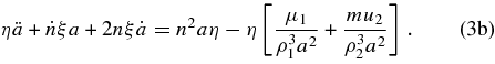
Following Murray (1994), we multiply Equation (3a) by η and subtract Equation (3b) times ξ, giving

$$\begin{equation} a^2(\dot{n}a+2n\dot{a}) = \mu _1\mu _2\frac{\eta }{\rho ^2} \left[\frac{1}{\rho _1^3}-\frac{1}{\rho _2^3}\right]. \end{equation} \tag{ 4 }$$

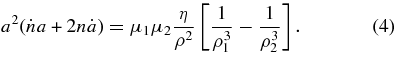
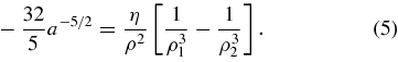
In the Keplerian limit, a = n^−2/3 and 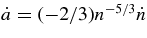$\dot{a}=(-2/3)n^{-5/3}\dot{n}$, so Equations (1d) and (4) give

$$\begin{equation} -\frac{32}{5}a^{-5/2} = \frac{\eta }{\rho ^2} \left[\frac{1}{\rho _1^3}-\frac{1}{\rho _2^3}\right]. \end{equation} \tag{ 5 }$$

In the limit of small μ₂, ρ ≈ ρ₁ ≈ 1 at the stable Lagrange points, and ρ₂ = (2 − 2cos ϕ_L)^1/2, giving

$$\begin{equation} \sin {\phi _L}\left(\frac{1}{(2-2\cos \phi _L)^{3/2}}-1\right) = \frac{32}{5}a^{-5/2}\,, \end{equation} \tag{ 6 }$$

where ϕ_L is the azimuth of the perturbed Lagrange point in the presence of GW losses (thus ξ = cos ϕ_L and η = sin ϕ_L). This relation is plotted as a dashed curve in Figure 2. Interestingly, the location of the Lagrange points is a function only of the binary orbital separation, not the mass ratio, even though the inspiral timescale is strongly dependent on μ₂. Note that, when including non-conservative forces such as GW evolution, there is a lack of symmetry between L₄ and L₅, with L₄ moving toward the secondary mass, while L₅ moves away from it. We also find differences in the relative stability of orbits around each Lagrange point, as described in the next section.

Zoom In Zoom Out Reset image size

In Figure 2, we plot the azimuthal position of test particles near L₄ and L₅ as a function of the binary separation a for a range of mass ratios. The initial binary separation is a₀ = 40M, and each curve represents a single test particle, initially at rest in the rotating frame, and placed at the location of the Newtonian Lagrange points. The test particles are evolved according to Equations (1a)–(1d), using a sixth-order Cash–Karp integrater with adaptive step size and accuracy of a part in 10¹⁰ (for a₀ = 40M, this corresponds to a maximum fractional error of ∼10⁻⁵ over the entire inspiral). For the most part, the test particles remain very close to their initial locations throughout inspiral, evolving according to Equation (6). While our Newtonian equations of motion do not formally predict an innermost stable circular orbit (ISCO), we expect the BHs to plunge and merge around a = 5M, at which point very little evolution in ϕ_L has taken place. In Figure 2, the slight offsets in the various curves at large a are due to the fact that ϕ is measured with respect to the origin, not M₁ (indeed, plotting ϕ₁ instead of ϕ gives curves that lie exactly on top of each other; see Figure 1).

The inclusion of PN corrections to the equations of motion would likely change the shape of the curves in Figure 2 slightly, as well as the detailed shape of stability regions around L₄ and L₅ (Rosswog & Trautman 1996). It should be noted that Seto & Muto (2010) include only 1PN terms, and do find a significant reduction in stability for certain mass ratios. Yet due to the notoriously uneven convergence of most PN expansions (e.g. Buonanno et al. 2009 and references therein), it is not clear whether their inclusion would add significant physical insight to the problem. Furthermore, eccentric binary orbits could also reduce the stability of test particles in systems near the critical mass ratio (Erdi et al. 2009), but these eccentric systems may not be astrophysically common.

When studying inertial drag forces in planetary three-body systems, Murray (1994) found that the L₄ point was more stable than L₅. Since our problem is almost the mirror image of that one (i.e., the added $\dot{n}$ terms in Equations (1a) and (1b) have the same form, yet opposite signs of inertial drag terms), it is not surprising then that we find greater stability around L₅ when including GW evolution. As shown in the upper panel of Figure 2 for μ₂ = 0.038, a test particle initially very close to L₄ will eventually get ejected from the equilibrium configuration as the binary approaches merger. On the other hand, test particles librating around L₅ appear to become slightly more stable, approaching the exact equilibrium position for small a. As mentioned in Erdi et al. (2009), for binaries with μ₂ slightly above the critical value for linear stability (0.0385 ≲ μ₂ ≲ 0.0401), there still exist bound orbits that librate around L₄ and L₅ with moderate amplitude. We find that for these systems, the inclusion of radiation reaction maintains or even increases the stability of L₅ by damping the libration amplitude. On the other hand, the libration amplitude of particles around L₄ grows rapidly toward the end of inspiral. This can be seen in Figure 3, where we plot the average libration amplitude for test particles initially very close (δr/a ∼ 10⁻⁴) to the equilibrium points, for the linearly unstable case of μ₂ = 0.039. These test particles move rapidly away from equilibrium, then remain on bounded libration orbits with δr/a ∼ 0.1. The libration angle around L₅ is roughly constant during inspiral, with a small upturn at the very end. L₄ is clearly more unstable, with a significant increase in the libration amplitude for a ≲ 15M. In contrast, Seto & Muto (2010) find no difference between L₄ and L₅, although they only consider a few test particle orbits around each Lagrange point.

Zoom In Zoom Out Reset image size

To further investigate this asymmetry in stability, we carried out orbital integrations for large numbers of test particles distributed in clouds around each Lagrange point for masses μ₂ = 0.01, 0.02, and 0.038. This allowed us to probe the regions relatively far from the equilibrium points, where standard linear stability analysis breaks down. We used two methods for estimating the large-scale stability of orbits around each Lagrange point. The first was a simple number count: the fraction of particles that remain bound around the equilibrium point. In this context, a particle is considered bound if its instantaneous Jacobi constant C_J is less than C_J0(L₃) for the present orbital separation, corresponding to the tadpole-shaped regions around L₄ and L₅ in Figure 1. Additionally, any particle that escapes with r > 10a or approaches closer than 3μ₁ from the primary or 3μ₂ from the secondary is removed from the system. The second method of measuring stability was to calculate the total volume filled by bound particles around each Lagrange point, a metric that is closely related to the mean libration amplitude. A larger volume corresponds to lower stability, as the particles begin to escape the bound libration region.

The fraction of bound particles f_bound is plotted in the top panels of Figure 4, normalized to the bound number at binary separation of a = 35M. The particles begin in a small cloud of radius δR around each Lagrange point with random velocities, isotropic with 〈v〉 = v_orb(δR/a)^1/2 in the corotating frame. We select δR to be large enough so that the cloud of particles roughly fills the phase-space volume of stable orbits around L₄ and L₅. In practice, this typically corresponds to half of the particles getting ejected on roughly a dynamical time after the start of the simulation (hence f_bound is defined relative to a = 35M, not a = 40M). After a stable cloud is formed around each Lagrange point, marginally bound particles are slowly ejected from the system (or accreted onto one of the BHs) as the binary system evolves adiabatically. From Figure 2, we might expect more particles to get ejected from L₄, which appears to be less stable, at least at linear order. However, as evident in Figure 4, L₄ retains more bound particles when μ₂ = 0.01, L₅ appears more stable for μ₂ = 0.02, and they are nearly identical for μ₂ = 0.038.

Zoom In Zoom Out Reset image size

It is not entirely clear why this peculiar behavior occurs, with no apparent trend in global stability as a function of mass ratio, nor why one Lagrange point or the other should be more stable for a given mass ratio. As described in Murray & Dermott (1999), test particles near the stable Lagrange points move along epicycles with two distinct frequencies. For certain values of μ₂, these libration frequencies have integer commensurabilities, which naturally leads to strong resonant interactions (Deprit & Deprit-Bartholomé 1967). For example, when μ₂ = 0.0243, both L₄ and L₅ are stable under standard linear analysis, yet the two epicyclic frequencies have a ratio of 2:1, leading to resonant excitations and ejection of all test particles after a few dynamical times (Erdi et al. 2009; Seto & Muto 2010). Murray (1994) shows that these characteristic frequencies change in the presence of inertial drag forces, which are directly analogous to GW evolution. Thus, we suspect that the different behavior seen in f_bound(t) for different Lagrange points is due to a combination of resonant interactions and asymmetric shifts in the libration frequencies due to the binary evolution via GW losses.

In the middle row of Figure 4, we plot the rms libration amplitude, defined for a set of bound particles by their instantaneous positions (x_i, y_i, z_i):

$$\begin{equation} \langle \delta r\rangle _{\rm bound} \equiv \frac{1}{N_{\rm bound}}\sqrt{\sum _i (x_i-\bar{x})^2 + (y_i-\bar{y})^2 + (z_i-\bar{z})^2 }\,, \end{equation} \tag{ 7 }$$

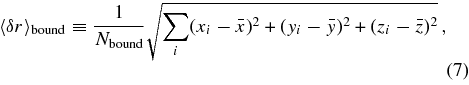
where the sum is taken over the test particles bound to either L₄ or L₅, and the mean positions $(\bar{x}, \bar{y}, \bar{z})$ are calculated over the same set. Closely related to 〈δr〉_bound, in the bottom panels of Figure 4 we plot the total volume V_bound occupied by bound particles, normalized to the overall scale of the binary a³. This volume is calculated by dividing the total simulation region into a large number (typically ∼10⁶) of small Cartesian cells, and then simply adding up the total number of cells that are occupied by at least one particle (typically ∼10⁴). We find this method to be independent of the number of cells or particles, as long as the average occupied cell has more than one particle, i.e., there are very few empty cells within the stable volume. In the limit of a very small δR/a, where the test particles are well within the linear regime, the cloud around each Lagrange point will actually expand adiabatically relative to the binary separation, although shrinking on an absolute scale. Fleming & Hamilton (2000) show this evolution scales as a^9/4:

$$\begin{equation} \left(\frac{V_f}{V_i}\right) = \left(\frac{a_f}{a_i}\right)^{9/4}, \end{equation} \tag{ 8 }$$

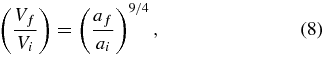
where V_i and V_f are the initial and final volumes of test particle clouds. We have confirmed this result numerically with simulations starting with δR ≪ a. On the other hand, if δR/a is large enough such that the stable region of phase space is completely filled, the normalized volume V/a³ should be constant, since the entire problem is scale invariant. Any adiabatic expansion will not increase the volume of bound orbits, but rather decrease the total number of particles in these regions, as seen in the upper panels of Figure 4.

We actually find a gradual increase in V_bound/a³ as the binary shrinks, yet still much slower than the Fleming & Hamilton (2000) result of (V/a³) ∼ a^−3/4, suggesting that the bound region in phase space is in fact filled. The increase in V_bound/a³ during the adiabatic inspiral phase (a ≳ 10M) is likely due to a combination of effects. First, we expect a net increase in global stability caused by the GW losses, analogous to the effects of inertial drag described in Murray (1994). Second, there is also some inherent error in measuring the volume of bound orbits, based on our crude metric of the test particles' instantaneous Jacobi constants. Some fraction of particles that have moved outside the stable region in phase space may still appear bound for a few dynamical times before getting ejected or accreted, and thus artificially contribute to V_bound.

At smaller a, where the libration time becomes comparable to the inspiral time, the system no longer evolves adiabatically, and a cloud of particles can get "frozen" at roughly constant volume, leading to the rapid increase in V_bound/a³ for a ≲ 10M. Interestingly, we do see a consistent trend of larger V_bound around L₄ than L₅ for all values of μ₂, as suggested by Figure 2. However, this may be less a measure of local stability than a consequence of the fact that L₄ moves toward the secondary, while L₅ moves away from it. Thus, the two regions begin to sample different potentials, and the gravitational force of the secondary acts to disrupt the cloud around L₄ more strongly than that around L₅, in turn leading to a larger V_bound.

We should add as a word of caution that many of these numerical stability results may be altered somewhat by the inclusion of additional PN terms to the equations of motion (Seto & Muto 2010). In general relativity, unlike the case of Newtonian gravity, test particles moving in the Kerr metric have three distinct epicyclic frequencies. These additional frequencies may lead to more complicated resonant interactions and thus change the behavior of f_bound(a) and V_bound(a), at least at a quantitative level. Yet our intuition suggests that the qualitative behavior shown in Figure 4 should remain unchanged, especially for mass ratios μ₂ ≲ 0.01 where resonance interactions are weaker. Future work will investigate this question in greater detail.

4.1. Formation Mechanisms

In the previous sections, we showed analytically and numerically how the location and stability of the L₄ and L₅ Lagrange points evolve in the presence of radiation reaction. We found that test particles, once captured into libration orbits around one of the stable Lagrange points, will in general remain there throughout the adiabatic inspiral phase, as the entire length scale of the system steadily shrinks. However, the initial premise was not addressed: will there even be gas or stars or debris present in the first place? How might matter get captured into these orbits at large binary separations? Furthermore, are binary BHs with μ₂ ≲ 0.04 astrophysically likely, or even possible?

Even in a system as well studied as the Sun–Jupiter binary, there is still no clear consensus on the origin of the Trojan asteroids, despite the fact that orbital elements are now known for over 4000 individual objects. Rabe (1972) proposed that they may be captured comets, while Shoemaker et al. (1989) and Kary & Lissauer (1995) suggested a more local origin as planetesimals in the early solar system. In most theories, some form of dissipative force is required to capture the Trojans (Yoder 1979), such as nebular gas drag (Murray 1994; Kary & Lissauer 1995) or planetesimal collisions (Shoemaker et al. 1989). Additionally, an increase in Jupiter's mass via accretion of the surrounding disk could lead to asteroids getting captured (Marzari & Scholl 1998; Fleming & Hamilton 2000). Analogous to our BH binary system, the inward migration of Jupiter may have also affected the capture and subsequent evolution of the Trojans (Yoder 1979; Fleming & Hamilton 2000).

The characteristic separation at which point a hard BH binary (i.e., the orbital potential is dominated by the two BHs, and not by the surrounding stars) is formed is comparable to the primary BH's radius of influence (Merritt 2006):

$$\begin{equation} a_{\rm h} = \frac{q}{(1+q)^2}\frac{R_{\rm infl}}{4}, \end{equation} \tag{ 9 }$$

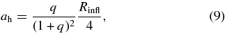
where q = M₂/M₁ and

$$\begin{equation} R_{\rm infl} = \frac{GM}{\sigma ^2} \approx 1.1\, {\rm pc}\, \left(\frac{M}{10^7\, M_\odot }\right)\left(\frac{\sigma }{200\, {\rm km}\, {\rm s}^{-1}}\right)^{-2}\,, \end{equation} \tag{ 10 }$$

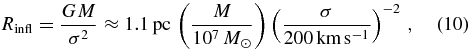
with σ being the one-dimensional velocity dispersion of the galaxy's bulge. In the limit of small μ₂ ≈ q ≪ 1, we have

$$\begin{equation} a_{\rm h} \approx 5\times 10^{-3}\, {\rm pc} \left(\frac{\mu _2}{0.02}\right) \left(\frac{M}{10^7\, M_\odot }\right)\left(\frac{\sigma }{200\, {\rm km}\, {\rm s}^{-1}}\right)^{-2}\,, \end{equation} \tag{ 11 }$$

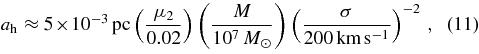
corresponding to a_h ∼ 10⁴M in geometrized units. Within this region, there are typically hundreds of stars (Hopman & Alexander 2006), and in active galactic nuclei (AGNs), a great deal of gas and dust as well. It is also roughly the separation at which point the binary will merge within a Hubble time due to GW losses alone (Peters 1964), and thus Equations (1a)–(1d) are appropriate.

For AGN with massive accretion disks, it is possible for significant star formation to occur in the region where the disk becomes self-gravitating (Levin & Beloborodov 2003). For standard thin disk models (Shakura & Sunyaev 1973), this self-gravitating radius actually corresponds closely to a_h. Since galaxy mergers are often associated with gas inflow and quasar activity, it is quite possible that stars could form in an accretion disk just as a hard BH binary is forming, thereby trapping the stars around the stable Lagrange points. A similar possibility, suggested by Goodman & Tan (2004), is that supermassive stars with M ≳ 10⁴ M_☉ could grow out of main-sequence seeds embedded in the accretion disk, quickly evolving and then collapsing to intermediate-mass black holes (IMBHs). This scenario is particularly attractive, as it naturally provides a mechanism for making a binary BH with μ₂ ≲ 0.01 and a circular orbit, surrounded by ample debris that could easily get trapped into resonant orbits.

Another mechanism that could explain both the low-mass secondary and also provide a supply of stars would be the tidal disruption of a globular cluster by the primary BH. If the globular cluster hosts an IMBH (Miller & Hamilton 2002), it could form a hard binary with the primary, and the surrounding stars could get captured into stable orbits around L₄ and L₅. At this point, it would be impossible to carry out any quantitative analysis of the relative rates and likelihoods of these different scenarios, considering the remarkable lack of observational evidence for even a single SMBH binary with orbit smaller than a_h. Rather, we might realistically hope to discover such a system with help from one of the EM signatures described below.

4.2. Tidal Disruptions of Stars

Tidal disruptions of solar-type stars by SMBHs are expected to occur at a rate of ∼10⁻⁴ yr⁻¹ per Milky Way-type galaxy (Wang & Merritt 2004), and are excellent tools for detecting otherwise-quiescent nuclei at cosmological distances (Lidskii & Ozernoi 1979; Rees 1988). Typical luminosities are comparable to the Eddington limit, and the timescale for the rise and subsequent decay of the light curve is on the order of weeks to months (Ulmer 1999; Halpern et al. 2004), which is ideal for detection by wide-field time-domain surveys such as Pan-STARRS⁴ or LSST⁵ (Gezari et al. 2009). Tidal disruptions have recently been proposed as tools for detecting BH mergers or recoiling merger remnants, in some cases long after the merger occurs (Komossa & Merritt 2008; Chen et al. 2009; Stone & Loeb 2010).

In our scenario, the main-sequence stars are captured into resonant motion around L₄ or L₅ at large separation (a ∼ a_h) and then move in closer to the primary as the binary separation slowly shrinks. A star of mass M_* and radius R_* will get disrupted when the tidal forces from the BH are comparable to the star's own self-gravity, which occurs at a distance R_td from the primary:

$$\begin{equation} R_{\rm td} \approx R_\ast \left(\frac{M_1}{M_\ast }\right)^{1/3}. \end{equation} \tag{ 12 }$$

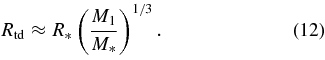
In our numerical tests of Section 3, we found that during inspiral, while some fraction of test particles get ejected from L₄ or L₅ and disrupted by M₂, the majority remain close to the Lagrange points until the final merger stage. For stars that remain bound to L₄ or L₅, the gravitational tidal forces are dominated by the primary, and thus the relevant mass in Equation (12) is M₁.

In Figure 5, we plot the orbital separation of a BH binary as a function of time before merger (black curves). The dashed horizontal lines correspond to the points at which (top to bottom) an O/B star, a solar-type star, or a white dwarf would get tidally disrupted by the primary BH of mass 10⁶ M_☉ (top) or 10⁷ M_☉ (bottom), and secondary mass μ₂ = 0.01. The vertical dotted lines denote when the binary separation reaches the ISCO and the BHs merge, and the vertical dashed lines correspond to the point where the binary enters the LISA GW frequency band. For M₁ = 10⁶ M_☉, a solar-type star would get disrupted roughly a year before merger (orphan planets of Jupiter or even Earth masses would actually get disrupted at a similar point, and could lead to comparably bright events, yet much shorter lived). At that point, LISA would already be able to provide an error box of ∼100 deg² for the source location on the sky (Lang & Hughes 2008), which could be easily monitored for luminous tidal disruption flares out to redshifts z ∼ 0.2 or so (Gezari et al. 2009). In all cases with M₁ ≳ 10⁵ M_☉, white dwarfs would not get disrupted, but rather plunge directly into the BH.

Zoom In Zoom Out Reset image size

In addition to the stars that get disrupted at late times, we found in the simulations of Section 3 that there are also some particles that get captured by either M₁ or M₂ during the inspiral phase, thus leading to tidal disruption, or get ejected entirely from the system. Table 1 shows the fraction of test particles that meet one of these various fates during inspiral, i.e., when the binary separation is 5M ⩽ a(t) ⩽ 35M. Of course, if Equation (12) is met, then even stars on stable orbits are disrupted. As in Figure 4, there are no clear trends with varying μ₂, but we do confirm that particles around L₅ are generally more likely to get ejected from the system, while particles around L₄ are more likely to get captured or disrupted by the BHs.

Table 1. Fraction of Test Particles that, During Inspiral, are Either Ejected from the System or Captured by One of the BHs

Fraction f	μ2 = 0.01	μ2 = 0.02	μ2 = 0.038
(L4 → ∞)	0.13	0.11	0.13
(L5 → ∞)	0.20	0.12	0.21
(L4 → M1)	0.16	0.33	0.19
(L5 → M1)	0.15	0.05	0.10
(L4 → M2)	0.14	0.27	0.18
(L5 → M2)	0.21	0.11	0.20

Download table as:  ASCIITypeset image

4.3. Ultra-hyper-velocity Stars

Of the stars that do get ejected from the binary system during inspiral, we find a wide range in their velocities at infinity. To first order, one would expect the ejection velocity to be comparable to the orbital velocity. However, particles ejected at late times when the orbital velocity is highest are also coming from the deepest potentials, so are slowed more as they escape from the system. In practice, we find that net effect is a slight increase in the average escape velocity at late times, but somewhat flatter than the orbital velocity scaling of a^−1/2. This is likely due to the fact that the most efficient three-body slingshot interactions require the test particle to come within a small fraction of a from the secondary, and when a becomes smaller, these close approaches more likely lead to capture or disruption than ejection.

From Equation (12), we see that a solar-type star would get tidally disrupted by a 10⁶ M_☉ BH at a distance of ∼50M, far outside the ISCO. For M₁ = 10⁷ M_☉, however, a star could survive to within 10M of the primary. In Figure 6, we show the distribution of velocity at infinity for a range of binary separations, with μ₂ = 0.02 and initial separation a₀ = 100M. As in Section 3, a cloud of test particles is chosen to roughly fill the stable regions around L₄ and L₅ at large a, then evolves with the binary, tracking which particles are ejected before the ISCO is reached. We see that, for a ≲ 50M, test particles can be ejected from the system with velocities of v_∞ > 0.1c, roughly 50 times greater than the radial velocities of HVSs observed in the outer regions of the Milky Way (Brown et al. 2009), and significantly larger than even the highest attainable values for main-sequence binaries getting disrupted by single SMBHs (Sari et al. 2010). Of course, any star moving that fast would be observable for a much shorter time; only a few million years after the BH merger. At the same time, this allows younger, more massive stars to survive out to the edge of the galaxy, making them even easier to identify against the field stars. It is conceivable that the BH at the center of our galaxy may have experienced a minor merger with μ₂ ∼ 0.01 in the past 10 Myr, an event which may be convincingly inferred by the detection of such an ultra-HVS at a distance of ∼50–100 kpc.

Zoom In Zoom Out Reset image size

4.4. Compressed Stellar Systems

4.5. Compact Objects

4.6. Diffuse Gas

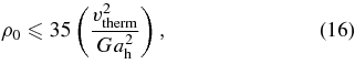
In the circumbinary accretion disk model, ample gas and dust will surround the BH binary, of which some fraction could likely get trapped into orbits around L₄ and L₅. If cold enough, this gas could get compressed by the evolving binary potential and form stars or even clusters of stars, as discussed above. More likely, the gas will be rather hot, with thermal velocities comparable to the libration velocities of test particles filling the stable volume around L₄ and L₅. One very rough estimate of this thermal motion may come from inspection of Equation (2) and Figure 1. Trapped particles will have C_J0(L₄) ≲ C_J ≲ C_J0(L₃), so typical velocities in the rotating frame of

$$\begin{equation} v^2 \approx C_{\rm J}(L_3,v=0)-C_{\rm J}(L_4,v=0)\approx 2\mu _2 a^{-1} \end{equation} \tag{ 13 }$$

(Murray & Dermott 1999). Combining with Equation (11) for the separation at the time of binary formation, we get an initial thermal velocity of

$$\begin{equation} v_{\rm therm} \approx 600\, {\rm km}\, {\rm s}^{-1} \bigg(\frac{\sigma }{200\, {\rm km}\, {\rm s}^{-1}}\bigg), \end{equation} \tag{ 14 }$$

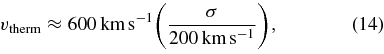
or roughly 4 × 10⁷ K. Somewhat remarkably, v_therm is independent of μ₂ or M₁ (except indirectly through the M–σ relationship).

We can estimate an upper limit on the density of this gas ρ₀ by requiring it to be stable to gravitational collapse. In other words, the total mass should not exceed the Jeans mass:

$$\begin{equation} 0.005\, \rho _0 a_{\rm h}^3 \le \left(\frac{5k_B T}{Gm_p}\right)^{3/2} \left(\frac{3}{4\pi \rho _0}\right)^{1/2}, \end{equation} \tag{ 15 }$$

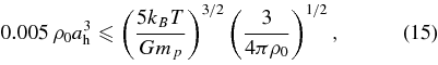
with k_B the Boltzmann constant and m_p the proton mass. The leading factor of 0.005 comes from the volume of the stable region, estimated from Figure 4. Taking m_pv²_therm = 3k_BT, we get

$$\begin{equation} \rho _0 \le 35 \left(\frac{v_{\rm therm}^2}{G a_{\rm h}^2}\right), \end{equation} \tag{ 16 }$$

corresponding to a total mass in gas of

$$\begin{equation} M_{\rm gas} \approx 0.005 \rho _0 a_{\rm h}^3 \le 7\times 10^4\, M_\odot \left(\frac{\mu _2}{0.02}\right) \left(\frac{M}{10^7\, M_\odot }\right)\,, \end{equation} \tag{ 17 }$$

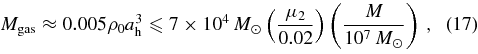
which is far more than enough material to fuel a bright EM counterpart.

Even if the density of the trapped gas is orders of magnitude smaller, it should still be sufficient to produce observable emission lines if irradiated by an AGN or quasar powered by accretion onto one of the BHs. For a cloud of gas filling the stable region around each Lagrange point, the covering fraction would be on the order of a few percent. Since the thermal velocity is roughly a factor of 10 smaller than the orbital velocity, the emission lines would be somewhat narrower than a classical broad line originating from the same radius. The coherent shape and motion of the cloud would also give rise to a large velocity offset relative to the host galaxy or narrow emission line clouds residing at a greater distance from the central engine. This offset in wavelength would vary periodically with the binary orbit (T_orb at our fiducial value of a_h would be on the order of 10 years), giving strong evidence for the existence of a BH binary. Such an effect could be detected by large spectroscopic surveys like the Sloan Digital Sky Survey, a technique already in frequent use by observers searching for binary quasars or recoiling BHs (Bonning et al. 2007; Komossa et al. 2008; Boroson & Lauer 2009).

We have analyzed the circular restricted three-body problem including leading-order terms for GW losses, in particular studying the behavior of test particle orbits near the stable Lagrange points L₄ and L₅. We find that these orbits remain stable throughout most of the adiabatic inspiral phase, and their locations shift relative to the Newtonian limit as the binary enters the late phases of inspiral and merger. Analogous to the case of inertial drag forces in the planetary problem, the non-conservative GW loss terms lead to an asymmetry between L₄ and L₅: test particles around L₄ move closer to the secondary BH, while those initially around L₅ move away from it. While there appear to be complicating resonances that affect the relative stability of the two regions differently for different mass ratios, a general trend is that the inclusion of GW losses increases the stability of L₅ while decreasing the stability of L₄. Particles initially around L₄ are more likely than those around L₅ to get captured or disrupted by M₁ or M₂, while particles near L₅ are more likely to get ejected from the system entirely. However, in both cases, the vast majority of particles neither get ejected nor captured until the binary separation is on the order a ≲ 5M, at which point the Newtonian equations of motion break down entirely and everything plunges into the primary BH.

The stability of the L₄ and L₅ Lagrange points throughout most of the inspiral provides a natural mechanism for shepherding material from relatively large radii down to the central BH, in turn producing a luminous EM counterpart to the GW signal from a BH merger. The detailed physics behind such an EM signal are well beyond the scope of this paper, but early results from NR simulations suggest that bright EM flares should be quite general, provided enough gas is available (van Meter et al. 2010; Bode et al. 2010; Farris et al. 2010). In addition to the prompt emission associated with the final merger, we have shown that HVSs with speeds as high as 0.1–0.2c might be observable, flying away from the galactic center for millions of years after the merger. With sufficient column densities of diffuse gas trapped around L₄ and L₅, a precursor signal could take the form of highly red/blueshifted emission lines, narrower than typical broad lines, with the line offset varying periodically with the BH orbit.

For the majority of the results in this paper, we require that the secondary mass be relatively small: μ₂ ⩽ 0.0385 to guarantee linear stability of L₄ and L₅. It is unclear how common BH binaries with such mass ratios might be, and whether they are more likely to form via galactic minor mergers or in situ, via the collapse of supermassive stars, accretion from a surrounding disk, or capture from a tidally stripped globular cluster. However, there are other resonances in the restricted three-body problem that may lead to qualitatively similar behavior: the stable transport of matter from large radii down to the ISCO at the time of merger. One example from the solar system is the Hilda family of asteroids that occupy stable eccentric orbits with periods 2/3 that of Jupiter. This ensures that they avoid close encounters with Jupiter at apocenter, where they spend most of their time. In the corotating frame, their trajectories trace out a triangle with vertices aligned with L₃, L₄, and L₅ (Brož & Vokrouhlický 2008). Guéron (2006) showed that this 2:3 resonance is stable even in the extreme relativistic limit, but still with small mass ratios (μ₂ ≈ 0.001). Our own preliminary results suggest that the Hilda resonance orbits are linearly stable for mass ratios at least as large as μ₂ ≈ 0.1, but we leave a comprehensive study of the problem, including GW losses, to a future paper.

In addition to all the Newtonian resonance behavior present in the three-body problem, the two BHs may also get locked into spin–orbital resonances with each other during inspiral (Schnittman 2004). Coupled with the non-degenerate orbital frequencies of test particles in a Kerr background, the inclusion of spinning BHs would introduce many new degrees of freedom that may affect the stability of L₄ and L₅. While we do not think additional PN terms in the equations of motion will significantly change our results on a qualitative level, future work that addresses these questions in more detail is certainly warranted. Another important complication would be the inclusion of eccentricity. While BH binaries are expected to circularize during the inspiral phase due to GW emission, they may be born with significant eccentricities. As shown in Erdi et al. (2009), eccentricity generally lowers stability around L₄ and L₅, especially near the critical mass ratio μ₂ ≳ 0.02.

The author thanks Doug Hamilton, Matthew Holman, Scott Hughes, Julian Krolik, David Merritt, and Cole Miller for helpful discussions and comments. The anonymous referee provided invaluable comments and suggestions. This work was supported by the Chandra Postdoctoral Fellowship Program.