


ABSTRACT
Recent measurements of hot and cold spots on the cosmic microwave background (CMB) sky suggest the presence of super-structures on (>100 h−1 Mpc) scales. We develop a new formalism to estimate the expected amplitude of temperature fluctuations due to the integrated Sachs–Wolfe (ISW) effect from prominent quasi-linear structures. Applying the developed tools to the observed ISW signals from voids and clusters in catalogs of galaxies at redshifts z < 1, we find that they indeed imply a presence of quasi-linear super-structures with a comoving radius of 100 ∼ 300 h−1 Mpc and a density contrast |δ| ∼ O(0.1). We also find that the observed ISW signals are at odds with the concordant Λ cold dark matter model that predicts Gaussian primordial perturbations at ≳3σ level. We confirm that the mean temperature around the CMB cold spot in the southern Galactic hemisphere filtered by a compensating top-hat filter deviates from the mean value at ∼3σ level, implying that a quasi-linear supervoid or an underdensity region surrounded by a massive wall may reside at low redshifts z < 0.3 and the actual angular size (16°–17°) may be larger than the apparent size (4°–10°) discussed in literature. Possible solutions are briefly discussed.
Export citation and abstract BibTeX RIS
1. INTRODUCTION
Although the Λ cold dark matter (CDM) models have succeeded in explaining a number of observations, some problems remain unresolved. For example, origins of a possible break of statistical isotropy in the large-angle cosmic microwave background (CMB) anisotropy (Tegmark et al. 2003; Eriksen et al. 2004; Vielva et al. 2004) and a possible discrepancy between observed and theoretically predicted galaxy-CMB cross-correlation (Rassat et al. 2007; Ho et al. 2008) are still not understood well. These observational results imply that structures on scales larger than ≳100 Mpc (super-structures) in our local universe are more lumpy than expected (Afshordi et al. 2009).
As the origin of the large-angle CMB anomalies, many authors have considered the possibility that the CMB is affected by local inhomogeneities (Moffat 2005; Tomita 2005a, 2005b; Cooray & Seto 2005; Rakić & Schwartz 2007). Inoue & Silk (2006, 2007) have shown that a particular configuration of compensated quasi-linear supervoids can explain most of the features of the anomalies. Subsequent theoretical analyses have shown that the CMB temperature distribution for quasi-linear structures can be skewed toward low temperature due to the second-order integrated Sachs–Wolfe (ISW, or Rees–Sciama) effect (Tomita & Inoue 2008; Sakai & Inoue 2008).
In fact, Granett et al. (2008) found a significant ISW signal on the scale of 4°–6° at redshifts around z ∼ 0.5 and a weak signal of negatively skewed temperature distribution for distinct voids and clusters at redshifts 0.4 < z < 0.75. Moreover, Francis & Peacock (2010) have shown that the ISW effect due to local structures at redshift z < 0.3 significantly affects the large-angle CMB anisotropies and that some of the CMB anomalies no longer persist after subtraction of the ISW contribution. These observations of galaxy–CMB cross-correlation may suggest an existence of anomalously large perturbations or new physics on scales >100 Mpc.
In order to evaluate the significance of the ISW signals for prominent structures, N-body simulations on cosmological scales seem to be suitable (Cai et al. 2010) for this purpose. However, the computation time is relatively long and finding physical interpretation from a number of numerical results is sometimes difficult. In contrast, analytical methods are suitable for estimating the order of statistical significance in a relatively short time, and physical interpretations are often simpler.
In this paper, we evaluate the statistical significance of the ISW signals for prominent super-structures based on an analytic method and try to construct simple models that are consistent with the data. In Section 2, we develop a formalism for analytically calculating the ISW signal due to prominent nonlinear super-structures based on a spherically symmetric homogeneous collapse model and we study the effect of nonlinearity and inhomogeneity of such structures. In Section 3, we apply the developed method to observed data and calculate the statistical significance of the discrepancy between the predicted and the observed ISW signals. In Section 4, we discuss the origin of the observed discrepancy. In Section 5, we summarize our results and discuss some unresolved issues. In the following, unless noted, we assume a concordant ΛCDM cosmology with (Ωm,0, ΩΛ,0, Ωb,0, h, σ8, n) = (0.26, 0.74, 0.044, 0.72, 0.80, 0.96), which agrees with the recent CMB and large-scale structure data (Sánchez et al. 2009).
2. CROSS CORRELATION FOR PROMINENT QUASI-LINEAR STRUCTURES
2.1. Thin-shell Approximation
For simplicity, in this section, we assume that super-structures are modeled by spherically symmetric homogeneous compensated voids/clusters with an infinitesimally thin shell. The background spacetime is assumed to be a flat FRW universe with matter and a cosmological constant Λ.
Let κ and ξ be the curvature and the physical radius of a void/cluster in unit of the Hubble radius H−1, and δH as the Hubble parameter contrast, t denotes the cosmological time. We describe the angle between the normal vector of the shell and the three dimensional momentum of the CMB photon that leaves the shell by ψ. We assume that the comoving radius rv of the void in the background coordinates satisfies rv ∝ tβ, where β is a constant.
Up to order O((rv /H−1)3) and O(κ2), the temperature anisotropy of the CMB photons that pass through spherical homogeneous compensated voids in the flat FRW universe can be written as (Inoue & Silk 2007)
where δm and Ωm denote the matter density contrast of the void and the matter density parameter, respectively. The variables ξ, ψ, δm , δH , and Ωm are evaluated at the time the CMB photon leaves the shell. It should be noted that formula (1) is valid even if |δm | or |δH | is somewhat large as long as the normalized curvature κ is sufficiently small. Formula (1) can be also applied to spherical compensating clusters with a density contrast δm > 0 corresponding to a homogeneous spherical cluster with an infinitesimally thin "wall." This approximation holds only in weakly nonlinear regime since the amplitude of the density contrast corresponding to a negative mass cannot exceed 1. We examine this approximation in Sections 2–4 in detail.
Because we are mainly interested in linear |δm | ≪ 1 and quasi-linear |δm | = O(0.1) regime, we expand δH in terms of δm up to the second order as

where w is an equation-of-state parameter,  is a constant that describes the nonlinear effect and
where 2
F1 is Gauss' hypergeometric function. can be estimated from numerical integration of the Friedmann equation inside the shell as we shall show later. In a similar manner, for the shell expansion, we assume the following relation for the wall peculiar velocity normalized by the background Hubble expansion
where ν represents a constant that describes the nonlinear effect (Inoue & Silk 2007). f(Ωm ) is written in terms of the scale factor a and the growth factor D as
In quasi-linear regime, simplification = η = 0 can be verified, which will be shown in Sections 2.3 and 2.4.
2.2. Homogeneous Collapse
In order to describe the dynamics of local inhomogeneity, we adopt a homogeneous collapse model which consists of an inner FRW patch and a surrounding background flat FRW spacetime (Lahav et al. 1991). The size of the inner patch is assumed to be sufficiently smaller than the horizon H−1 in the background spacetime.
We assume that both the regions have only dust and a cosmological constant Λ. The time evolution of either the inner patch or the background spacetime is described by the Friedmann equation
where a denotes the scale factor, Ωm,0, ΩΛ,0, Ωtot are the present energy density parameters of non-relativistic matter, a cosmological constant Λ, and the total energy density, respectively. The scale factor at present for the background spacetime is set to a0 = 1. In what follows, we describe variables in the inner patch by putting tilde "∼" on top of the variables and we consider only flat FRW universes with dusts and a cosmological constant Λ.
First, we calculate matter density contrast δm
of the inner patch. Initially (zi
≫ 1), we assume that the fluctuation of the matter perturbation δmi
is so small that  . Then, the Friedmann equation (Equation (7)) yields
In terms of physical radius of the patch  , where r is the comoving radius measured in the background spacetime, Equation (8) can be written as
where t is the cosmological time. The matter density contrast δm can be written as a function of a ratio of the present and the initial comoving radius η ≡ r/ri as δm = η−3 − 1. From Equation (9), η as a function of redshift z is given by solving
Note that right-hand side in Equation (10) does not depend on  . From numerical integration of Equation (10), the matter density contrast δm
as a function of redshift z is obtained by setting initial density contrast δmi
= δm
(zi
).
. From numerical integration of Equation (10), the matter density contrast δm
as a function of redshift z is obtained by setting initial density contrast δmi
= δm
(zi
).
The linearly perturbed matter density contrast δL m in the FRW background spacetime is given by
where H2(z) = Ωm,0(1 + z)3 + ΩΛ,0 (Heath 1977). Constant 3/5 comes from our choice of initial condition that the peculiar velocity inside the initial patch is zero. The relation between δm and δL m is shown in Figure 1.
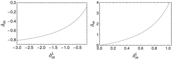
Figure 1. Density contrast δm as a function of linear density contrast δL m for voids (left) and clusters (right).
Download figure:
Standard image High-resolution imageBecause the relation does not change much even if one varies the cosmological parameters of the background spacetime, nonlinear isolated homogeneous spherical patches can be solely calculated from corresponding linear perturbations (Friedmann & Piran 2001). It should be noted, however, that the relation is valid only if δm ≳ δv,cut = −0.8 because of shell crossing (Furlanetto & Piran 2006).
Next, we calculate the Hubble parameter contrast  in nonlinear regime. Plugging η = R(1 + z)/(Ri
(1 + zi
)) into Equation (8), we have
in nonlinear regime. Plugging η = R(1 + z)/(Ri
(1 + zi
)) into Equation (8), we have
where η is given by solving Equation (10). From Equations (3) and (12), one can estimate the nonlinear parameter as

2.3. Effect of Nonlinear Dynamics
In the previous section, we have seen that the nonlinear density contrast δm
for a spherically symmetric homogeneous patch can be written in terms of corresponding linear density contrast δL
m
. In order to calculate the ISW effect, we need to estimate the Hubble parameter contrast δH
and the peculiar velocity  of the wall. The nonlinear corrections to δH
and
of the wall. The nonlinear corrections to δH
and  can be characterized by two parameters and ν, respectively.
First, we consider the effect of nonlinear correction to the Hubble contrast δH
. As one can see in Figures 2 and 3, is always negative and the amplitude is || < 0.16 for |δm
| < 1.0. This represents a slight enhancement in the expansion speed within the inner patch due to nonlinearity. In low-density universes (Ωm,0 < 1), || is smaller than that in high-density universes. In the Einstein–de Sitter (EdS) universe, depends only on δm
(Figure 2). In contrast, in low-density universes, depends on the amplitude of the initial epoch as well (Figure 3). This is because the expansion speed inside the patch is suppressed when the energy component of the background universe is dominated by a cosmological constant Λ. We have found that the nonlinear contribution to δH
is less than 10% for |δm
| < 0.2 and Ωm
> 0.26.
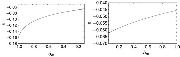
Figure 2. Nonlinear parameter as a function of density contrast δm
in the EdS model.
Download figure:
Standard image High-resolution image
Figure 3. Nonlinear parameter as a function of density contrast δm
in the flat-Λ model with Ωm,0 = 0.26.
Download figure:
Standard image High-resolution imageSecond, we consider the effect of the nonlinear correction to the peculiar velocity of the wall. In the thin-shell limit, the motion of the spherically symmetric wall can be obtained by numerically solving a set of ordinary differential equations using Israel's method (Israel 1966; Maeda & Sato 1983). If the inner region and the outer region are described by the FLRW spacetime, the fitting formula for the peculiar velocity of an expanding wall normalized by the background Hubble expansion can be written as (K. Maeda et al. 2010, in preparation)
for Ωm
+ ΩΛ = 1. We have confirmed that the accuracy of the fitting formula is within 1% for 0 < Ωm
⩽ 1 and |δm
| < 1 using numerically computed values. From Equation (14), we find that the contribution of the nonlinear effect is less than 5% for |δm
| < 0.3. Thus an approximation  can be validated in the quasi-linear regime.
2.4. Effect of Nonlinearity and Inhomogeneity on the ISW Signal
In literature, the thin-shell approximation has been often used to describe almost empty voids with δ ∼ −1 (Maeda & Sato 1983). In quasi-linear regime, however, we also need to consider the effect of thickness of the wall and inhomogeneity of the matter distribution because quasi-linear voids are not in the asymptotic regime. Nonlinearity of the wall may significantly affect the CMB photons that pass through it. Moreover, it seems not realistic to apply the thin-shell approximation to spherically symmetric clusters since the mass of the wall cannot be negative.
In order to estimate the validity of the thin-shell approximation, we have compared the ISW signal with those obtained by using the second-order perturbation theory (Tomita & Inoue 2008) and by using the Lemaitre–Tolman–Bondi (LTB) solution (Sakai & Inoue 2008), which yields exact results without recourse to the cosmological Newtonian approximation. We have assumed top-hat-type matter distribution (for linear matter perturbation) for void/cluster for calculation using second order perturbation theory and a smooth distribution specified by a certain polynomial function for calculation using the LTB solution. The voids/clusters are assumed to be compensated so that the gravitational potential outside the cutoff radius (r1 for the perturbative analysis and rout for the LTB-based analysis) is constant. For detail, see Appendices A and B.
As an example, we have computed temperature fluctuations ΔT generated from a compensated void/cluster using the three types of methods. The density contrast, the comoving radius and the redshift of the center of a void/cluster are set to |δm | = 0.1, rv = 200 h−1 Mpc, r1 = rout = 210 h−1 Mpc, and z = 0.2, respectively. The width of the wall is assumed to be 1/10 of the cutoff radius. As one can see in Figure 4, the three methods agree well for low density universes in which the linear effect is dominant. In contrast, the discrepancy becomes apparent for high density universes in which the nonlinear effect is dominant. This discrepancy is partially due to a slight difference in the assumed density profile (top-hat-type for the perturbative analysis, polynomial type for the LTB). In order to demonstrate the role of nonlinearity, we have plotted the first-order (linear ISW effect) and the second-order (RS effect minus linear ISW effect) contributions to the ISW signal (Figure 5). The first-order effect makes the CMB temperature negative (positive) for a void (cluster) but the second-order effect makes the CMB temperature negative near the center and positive near the boundary regardless of the sign of the density contrast. As a result, the amplitude of temperature fluctuation for a void (cluster) is enhanced (suppressed) in the direction near the center but it is suppressed (enhanced) in the direction near the boundary. These nonlinear effects become much more apparent for models with higher background density because the linear ISW effect becomes less effective. However, if we take into account the thickness of the wall, these nonlinear effects can be less conspicuous since the amplitude of the gravitational potential becomes smaller for a fixed outer radius (Figure 6). In the Λ-dominated universe, a quasi-linear compensated void can be recognized as a cold spot surrounded by a very weak hot ring, whereas a quasi-linear compensated cluster can be recognized as a hot spot possibly with a dip at the center of it. In the EdS universe, either a compensated quasi-linear void or a cluster can be identified as a cold spot surrounded by a hot ring.

Figure 4. Temperature fluctuation ΔT due to a compensated cluster (left panels)/a compensated void (right panels) centered at redshift z = 0.2 as a function of the angular radius from the center. We used three methods for deriving the ISW signal: the thin-shell approximation (thick curve), the second-order perturbation theory (dotted curve), and the LTB solution (dashed curve). We set the comoving (outer) radius of the cluster/void rv = 200 h−1 Mpc for the thin-shell approximation, rout = 210 h−1 Mpc for the second order and the LTB calculations with wall width about tenth of the outer radius. The density parameter is Ωm0 = 0.26. For details, see the text.
Download figure:
Standard image High-resolution image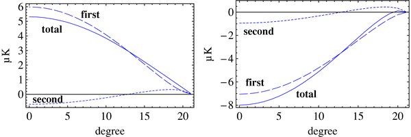
Figure 5. First and the second-order contributions to temperature fluctuation ΔT due to a compensating cluster (left)/void (right) centered at redshift z = 0.2 as a function of the angular radius from the center. We set the outer comoving radius rout = 210 h−1 Mpc, the inner comoving radius rin = 0.93 rout, the density parameter Ωm0 = 0.6, and the density contrast at the center of the cluster/void |δm (z = 0.2)| = 0.1.
Download figure:
Standard image High-resolution image
Figure 6. Effect of the thickness of the wall for Ωm0 = 0.6 r1 = 210 h−1 Mpc, and δm (z = 0.2) = 0.2 (left) and δm (z = 0.2) = −0.2 (right) for top-hat-type density perturbations (see Appendix A).
Download figure:
Standard image High-resolution image2.5. ISW Effect from Prominent Quasi-linear Structures
In order to fully utilize information of the three dimensional distribution, we consider a temperature anisotropy ΔT/T obtained from stacked images on the CMB sky that corresponds to most prominent voids/clusters in a galaxy catalog. First, we fix an angular radius θout of a circular region on the CMB sky that will be used in the stacking analysis. Then, the corresponding smoothing scale rs in comoving coordinate for the corresponding fluctuation at z is rs = (1 + z)DA (z)θout, where DA (z) is the angular diameter distance to the galaxy. The corresponding initial smoothing scale is ri s = η−1 rs .
We assume that the probability distribution function (PDF) of linear density contrast δL m at redshift z is given by a Gaussian distribution function
where σ2(ri s , z) is the variance of the linearly extrapolated density contrast at redshift z smoothed by a spherically symmetric top-hat-type window function with an initial comoving radius ri s . Note that σ(ri s , z) depends on cosmological parameters such as Ωm,0, σ8 and the spectrum index n. Then, the PDF of nonlinear density contrast of the inner patch δm is given by
where α is a constant that normalizes the PDF.
As shown in Figure 7, the PDF of δm is positively skewed in comparison with the PDF of δL m because of nonlinearity. For a sample region at redshift z with a total comoving volume V, the total number of voids or clusters with a radius rs is approximately Nt ≈ 3V/(4πr3 s ). In what follows, we assume that the number of prominent voids/clusters (Nv /Nc ) determines the corresponding threshold of density contrast δm,th (z), which is given by
and
respectively. From Equations (1), (17), and (18) the mean temperature fluctuation within an angular radius θout for a stacked Nv or Nc images corresponding to prominent quasi-linear voids/clusters at redshift ∼z can be approximately written as
where 0 ⩽ θ ⩽ θout, W(θ; θin) is a compensating window function that satisfies
and

where h = rs (1 + z)/DA (z).
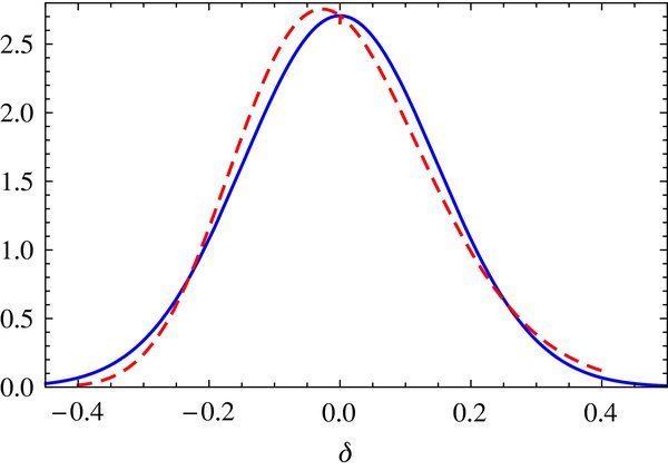
Figure 7. Effect of nonlinearity: the PDF of δm (dashed curve) and that of δL m (full curve) for a smoothing scale rs = 50 h−1 Mpc at z = 0.5.
Download figure:
Standard image High-resolution image3. APPLICATION TO OBSERVATIONS
3.1. SDSS–WMAP Cross Correlation
A cross correlation analysis using a stacked image built by averaging the CMB surrounding distinct voids/clusters has been done by Granett et al. (2008). They have used 1.1 million luminous red galaxies (LRGs) from the Sloan Digital Sky Survey (SDSS) catalog covering 7500 deg2. The range of redshifts of the LRGs is 0.4 < z < 0.75, with a median of ∼0.5. The total volume is ∼5 h−3 Gpc3. They used the so-called ZOBOV (ZOnes Bordering On Voidness; Neyrinck 2008) algorithm to find supervoids and superclusters in the LRG catalog and made a stacked image from an inversely variance weighted WMAP 5 year (Q, V, and W) map. In order to reduce contribution from CMB fluctuations on scales larger than the objects, they used a top-hat-type compensating filter
where θout = cos−1(2cos θin − 1).
First, using the developed tools based on thin-shell approximation and homogeneous collapse model in Section 2, we estimate the expected amplitude of the ISW signal for prominent structures in a concordant ΛCDM model with Gaussian primordial fluctuations and compare with the observed values obtained from the SDSS–LRG catalog. The number of most distinct voids or clusters N and the cutoff radius θin are chosen as free parameters. At redshift z = 0.5, the mean density contrast filtered by a top-hat-type function with radius r = 130 h−1 Mpc corresponding to θout ∼ 5 6 is just 〈δL
m
〉 = 0.046 and the background density parameter is Ωm
(z = 0.5) = 0.54. Because the influence of non-linear ISW effect is weaker than that of the linear ISW effect in this setting, we expect that details of nonlinear calculations will not affect the result much. In what follows, we use an approximation
6 is just 〈δL
m
〉 = 0.046 and the background density parameter is Ωm
(z = 0.5) = 0.54. Because the influence of non-linear ISW effect is weaker than that of the linear ISW effect in this setting, we expect that details of nonlinear calculations will not affect the result much. In what follows, we use an approximation  , where δm
is determined from the homogeneous collapse model in Section 2.
, where δm
is determined from the homogeneous collapse model in Section 2.
As shown in Table 1, it turned out that the expected values of the ISW (Rees–Sciama) signal are typically of the order of O(10−7) K. As expected, the amplitude gets larger as the number of stacked image decreases, and the amplitude for voids systematically becomes larger than those for clusters by 5%–10% (Tomita & Inoue 2008; Sakai & Inoue 2008). On the other hand, the order of the observed amplitudes are extremely large as O(10−6) K. It turns out that the discrepancy remains at 3σ–4σ level for N = 30 and N = 50.
Table 1. Expected and Observed Amplitude of Mean Temperature for a Compensating Filter θin = 4°
| N | Cluster (μK) | Void (μK) | Average(μK) |
|---|---|---|---|
| 1 | 0.98 | −1.2 | 1.07 |
| 5 | 0.82 | −0.94 | 0.88 |
| 10 | 0.73 | −0.83 | 0.78 |
| 30 | 0.57 | −0.64 | 0.61 (11.1 ± 2.8) a |
| 50 | 0.48 (7.9 ± 3.1) a | −0.53 (−11.3 ± 3.1) a | 0.51 (9.6 ± 2.2) a |
| 70 | 0.42 | −0.46 | 0.42 (5.4 ± 1.9) a |
Note. aTaken from Granett et al. (2008).
Download table as: ASCIITypeset image
Second, we reconstruct the mean density profile from the observed ISW signal for the SDSS–LRG catalog using our LTB model. From Figure 7, one can notice a hot ring around a cold spot for the stacked image of voids and a dip at the center of a hot spot for the stacked image of clusters. Although the amplitude of the hot-ring cannot be reproduced well, the observed dip at the center of the hot spot can be qualitatively reproduced in our LTB models. We have found that the dip at the center of a compensated cluster can be generated only if the linear ISW effect balances the nonlinear ISW effect in a limited parameter region. Thus the observed features in stacked images strongly imply that the corresponding super-structures are not linear but quasi-linear or nonlinear objects. The density fluctuations which are necessary to produce the observed ISW signals are found to be tremendously large. In Figure 8, we plot the ISW signal from a compensated cluster with δm ∼ 7σ and that from a compensated void with |δm | ∼ 10σ at z = 10 (see the radial density profiles in Figure A1 in Appendix A). Even for these very rare objects, the amplitudes of ISW signals in our LTB models are much smaller than the observed ones. In fact, the mean temperatures for a compensating filter θin = 4° are 3.6 μK(1.4σ) and −3.1 μK(2.6σ) for the cluster and the void, respectively. On the other hand, the probability of generating these fluctuations is as extremely small as 10−12 in standard inflationary models that predict primordial Gaussianity.
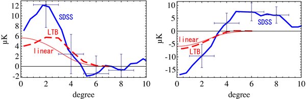
Figure 8. Observed mean CMB temperature radial profiles for a stack image of 50 clusters (left) and that of 50 voids (right, thick full curves) in the SDSS–LRG catalog (Granett et al. 2008) and the corresponding theoretical radial profiles for compensated spherical clusters (left)/void (right) based on the LTB solution (dashed curves) and the linear calculation (thin full curves) with a top-hat-type compensated density distribution corresponding to the LTB solutions. The LTB parameters for the set of clusters are (rout, rin, δm , zc ) = (0.055 H−1 0, 0.022 H−1 0, 1.0, 0.5) and those for the set of voids are (0.050 H−1 0, 0.015 H−1 0, − 0.55, 0.5). The effective radii of the inner patch at a redshift z = 10 and the mean filtered temperature with θin = 4° are (0.029 H−1 0, 3.6 μK) (cluster) and (0.023 H−1 0, − 3.1 μK) (void), respectively. Evolution of the density profile in the LTB models are shown in Appendix B. 1σ error bars are obtained from 1000 Monte Carlo simulations on the WMAP7 Q+V+W map smoothed at 1° scale (see Section 3.3).
Download figure:
Standard image High-resolution imageThus, the observed large ISW signals for the stacked image strongly suggest a presence of super-structures on scales O(100 h−1 Mpc) with anomalously large density contrast O(0.1) which cannot be produced in the concordant LCDM model.
3.2. 2MASS–WMAP Cross Correlation
Francis & Peacock (2010) estimated the local density field in redshift shells using photometric redshifts for the Two Micron All Sky Survey (2MASS) galaxy catalog. They reconstructed the CMB anisotropies due to the ISW effect from the local density field δm . They approximated the bias in each redshift shell by a linear bias relation δg = b δm and assumed that the bias is independent of scale and redshift in each shell. In order to obtain the bias parameter b, a maximum likelihood analysis of the galaxy catalog was performed.
There are two prominent spots in the reconstructed CMB anisotropy. One is a hot spot due to a supercluster around the Shapley concentration at redshifts 0.1 ⩽ z ⩽ 0.2. Another one is a cold spot due to a supervoid at redshifts 0.2 ⩽ z ⩽ 0.3 in the direction to (l, b) ∼ (0, − 30°). The angular radii of both structures are θ = 20°–30°. The temperatures near the center of both structures are ∼20 μK. The position of the supervoid is very close to the one predicted in Inoue & Silk (2007), (l, b) ∼ (330°, − 30°).
Based on the methods developed in Section 2, we have estimated the expected density contrast δm and the corresponding temperature profile (Figure 9) due to a most prominent object in the shell. We have assumed the same cosmological parameters and primordial Gaussianity as those discussed in Section 3. In order to compute the temperature profile, we have used a homogeneous thin-shell model. As shown in Table 2, the observed density contrasts are larger by 4–7 times the expected values. If the comoving radius of the structure is ∼200 h−1 Mpc, the absolute value of the density contrast should be |δm | = 0.2–0.3, which implies the presence of anomalous quasi-linear super-structures. Our result is consistent with the power spectrum analysis in Francis & Peacock (2010) where a noticeable excess of the observed power at low multipoles 2 ⩽ l ⩽ 4 was reported.
Figure 9. Left: theoretically modeled temperature profiles for an observed (full curves) and an expected (dotted curves) supercluster in the 2MASS catalog. Right: modeled temperature profiles for an observed (full curves) and an expected supervoid (dotted curves). These superstructures reside at redshifts z = 0.1–0.3. We have plotted two possible profiles for each structure since there is an ambiguity in the angular size due to errors (Δz ∼ 0.03) in photometric redshifts in the 2MASS galaxy catalog (Francis & Peacock 2010).
Download figure:
Standard image High-resolution imageTable 2. Expected and Observed Density Contrast for Super-structures in the 2MASS Galaxy Catalog
| Radius a | Expected | Observed | Radius a | Expected | Observed |
|---|---|---|---|---|---|
| 230 | 0.037 | 0.20 | 370 | −0.013 | −0.049 |
| 150 | 0.094 | 0.69 | 250 | −0.037 | −0.15 |
Note. aThe unit of the radii is h−1 Mpc.
Download table as: ASCIITypeset image
3.3. The CMB Cold Spot
The most striking CMB anomaly is the presence of an apparent cold spot in the Wilkinson Microwave Anisotropy Probe (WMAP) data in the Galactic southern hemisphere (Vielva et al. 2004; Cruz et al. 2005; see Figure 10). The cold spot has a less than 2% probability of being generated as random Gaussian fluctuations (Cruz et al. 2007a), if one uses spherical mexican-hat-type wavelets as filter functions (see also Zhang & Huterer 2010). Assuming that it is not a statistical artifact, a variety of theoretical explanations have been proposed, such as galactic foreground(Cruz et al. 2006), texture (Cruz et al. 2007b), and Sunyaev–Zeldovich (SZ) effect. However, these models failed to explain other large-angle anomalies by the same mechanism.
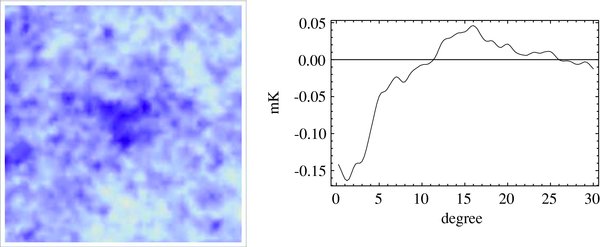
Figure 10. Left: the WMAP7 ILC temperature map (40° × 40°) smoothed at 1° scale. Right: the averaged radial profile of the ILC map as a function of inclination angle θ from the center of the cold spot (l, b) = (2078, − 563). A peak at θ ∼ 15° corresponds to a hot ring.
Download figure:
Standard image High-resolution imageInoue & Silk (2006, 2007) proposed that the cold spot may be produced by a supervoid at z < 1 in the line of sight due to the ISW effect and have shown that another pair of supervoids that are tangential to the Shapley concentration can explain the alignment between the quadrupole and the octopole in the CMB. Subsequently, Rudnick et al. (2007) found a depression in source counts in the NRAO VLA Sky Survey(NVSS) in the direction to the cold spot, although the statistical significance has been questioned (Smith & Huterer 2010). Recent optical observations (Granett et al. 2010; Bremer et al. 2010), however, revealed that any noticeable supervoids at 0.35 < z < 1 in the line-of-sight are ruled out. These observations suggest that the angular size of the supervoid may be larger or smaller than expected and that it resides at low redshifts z < 0.35 or at high redshifts z > 1.
In order to test such a possibility, we have calculated the average temperature around the cold spot (see Figure 11) using a spherical top-hat compensating filter Wth (θ; θin).

Figure 11. Left: 1σ of the filtered mean temperature as a function of an inner radius θin for the Q+V+W map (dashed curve) and that derived from Cl 's (thin curve) and from pseudo-Cl 's (thick curve). Right: 1σ for the ILC map (dashed curve) and corresponding theoretical values (thin curve and thick curve) as shown in the left figure.
Download figure:
Standard image High-resolution imageInterestingly, we have discovered two peaks in the plot of the filtered mean temperature around the cold spot as a function of inner radius of the filter (Figure 12). The inner and the outer peaks are observed at θin = 4°–5°(θout = 6°–7°) and θin = 12°–13° (θout = 16°–17°). The outer peak corresponds to a hot ring, which is visible by eyes (see Figure 10).
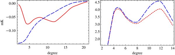
Figure 12. Left: mean temperature around the center of the cold spot for a compensating top-hat filter (full curve) and for an uncompensated top-hat filter without a ring (dashed curve) as a function of the inner radius θin. Right: mean temperature around the center of the cold spot divided by the standard deviation for the ILC map (dashed curve) and the Q+V+W map (full curve) as a function of θin.
Download figure:
Standard image High-resolution imageIn order to estimate the statistical significance of the peaks, we have used a WMAP 7 year internal linear combination (ILC) map smoothed at 1° scale with a Galactic sky cut |b| < 20° and a combination of the Q, V, and W band frequency maps smoothed at 1° scale averaged with weights inversely proportional to the noise variances with a "standard" Galactic sky cut made by the WMAP team. In order to reduce possible residual contamination from the Galactic foreground, we further cut a region |b| < 35° for the Q+V+W map. In order to estimate the errors, firstly, we generated 1000 random positions on the ILC(|b|>20°) and the Q+V+W(|b|>35°) maps, and then computed variances σ2 for the filtered mean temperature. Second, we have calculated expected σ2 for the filtered temperature using the angular power spectrum Cl for the WMAP 7 year data obtained by the WMAP team (see Appendix A). Note that we have computed pseudo-Cl 's from the Cl ' for each sky map. As shown in Figure 11, the observed standard deviations are 1σ = 19 ∼ 20 μK for θin = 4° and 1σ = 14 ∼ 16 μK for θin = 14°. Our result for θin = 4° is roughly consistent with the values for stacked images in Granett et al. (2008) assuming no correlation between voids/clusters in a particular configuration. In the Q+V+W map, a slight suppression in σ is observed at θin > 8°. Theoretically calculated values are found to be systematically lager than the observed values by 4%–16% for 4° < θin < 14°. These discrepancies represent an uncertainty due to the Galactic foreground emission.
As one can see in Figure 12, a deviation corresponding to the inner peak is roughly 4σ and that corresponding to the outer peak is 4 ∼ 4.5σ. Assuming that the filtered mean temperature obeys Gaussian statistics, the statistical significances are P(>4σ) = 6 × 10⁻³ and P(>4.5σ) = 7% × 10−4%. The total solid angle of the ILC map (|b|>20°) is 8.27 sr and that of the Q+V+W map (|b|>35°) is 5.36 sr. The total number of the independent patches is roughly given by a ratio between the solid angle of the map and the area of the spherical patch with angular radius θout. Therefore, for θout = 7°, we have ∼180 samples for the ILC and ∼110 samples for Q+V+W map, yielding (110–180) × P(>4σ) = 0.7%–1%. In a similar manner, for θout = 17°, one can easily show that the statistical significance is ∼0.01%–0.2% corresponding to ∼3σ if the likelihood function is a Gaussian one.
Thus, the cold spot surrounded by a hot ring at scale ∼17° is more peculiar than the cold spot at scale ∼7°. Therefore, the real size of the supervoid is expected to be larger than the apparent size of the cold region. Because 1σ deviation (corresponding to 15–20 μK) due to a supervoid is enough to make the signal non-Gaussian, it is reasonable to assume that the contribution from a supervoid is less important than that from other effects due to acoustic oscillation or Doppler shift at the last scattering surface. For instance, a supervoid with a density contrast δm = −0.3 with a comoving radius r = 200 h−1 Mpc at a redshift z = 0.2 corresponding to an angular radius θ = 20° would yield a temperature decrease ΔT ∼ 20 μK in the direction to the center. Moreover, if the supervoid is not compensating, a wall surrounding the supervoid could generate the observed hot ring. It may consist of just an ordinary underdense region surrounded by massive superclusters. Further observational study is necessary for checking the validity of the "local supervoid with a massive wall" scenario.
4. POSSIBLE SOLUTIONS
Why are the observed ISW signals for prominent structures so large?
One possible systematic effect may come from a deviation from spherically symmetric density profile that we have not considered. Indeed, gravitational instability causes pan-cake or needle like structures in high density regions. However, as we have seen, the order of the density contrast of relevant prominent super-structures is δm = O[0.1]. Therefore, we expect that the effect of anisotropic collapse plays just a minor role. Moreover, in the case of supervoids, a deviation from spherical symmetry is suppressed as the void expands in comoving coordinates. Thus, it is difficult to attribute the major cause to the deviation from spherical symmetry.
Another possible systematic effect is our neglect of fluctuations on larger scales. For instance, we may have observed just a tip of fluctuations whose real scale extends to r > 1000 h−1 Mpc. Indeed, the amplitude of the ISW effect is roughly proportional to the scale of fluctuations, i.e., ΔT/T ∝ r for r > 100 h−1 Mpc (Inoue & Silk 2007). Therefore, the observed large amplitude of ISW signal can be naturally explained. However, the angular sizes of the observed hot and cold spots from the stacked images are just 4°–6° at z ∼ 0.5 corresponding to r = 100–140 h−1 Mpc. It is difficult to explain why the angular sizes are so small since contributions from the ordinary Sachs-Wolfe effect and the early ISW effect generated near the last scattering surface are significantly suppressed by stacking a number of images.
Then what are the possible mechanisms that can explain the anomalously large ISW signals?
One intriguing possibility is that the primordial fluctuations are non-Gaussian. Our results suggest that the number of both supervoids and superclusters is significantly enhanced in comparison with the standard Gaussian predictions. Therefore, the effect of deviation from Gaussianity may appear in the statistics of four-point correlations in real space or trispectrum in harmonic space. It can be also measured by the Minkowski functionals that contain information of four-point or higher order correlations. At the last scattering surface, the comoving scale of 300 h−1 Mpc corresponds to angular scale ∼2°. If the background universe is homogeneous, such a non-Gaussian feature must appear at the CMB anisotropy at multiple l ∼ 100 corresponding to angular scale ∼2° as well. However, so far no such noticeable deviation from Gaussianity in the CMB anisotropies has been observed (Vielva & Sanz 2010). Therefore, it is difficult to explain the observed signals by a simple non-Gaussian scenario unless one gives up the cosmological Copernican principle (Tomita 2001).
Another possibility is a certain feature on the power spectrum of primordial fluctuation (Ichiki et al. 2010). Spike-like features in the primordial power spectrum appear in some inflationary scenarios that produce primordial black holes (Ivanov et al. 1994; Juan et al. 1996; Yokoyama 1998). Although there is no natural reason to have a feature only on the scale of super-structures (l ∼ 100), observational constraints are not stringent since one needs to increase the number of samples if one abandons the assumption of the smoothness of the primordial power.
Some cosmological models containing time evolving dark energy/quintessence or those based on scalar–tensor gravity predict an enhancement in the ISW effect due to an enhancement in acceleration of the cosmological expansion or non-trivial time evolution of dark energy or scalar field that may couple to matter or metric (Amendola 2001; Nagata et al. 2003). This may help explain the anomalously large ISW signal. However, at the same time, we need to suppress the ISW contribution on large angular scales since the observed angular power of the CMB anisotropy at very large angular scales l ∼ 2 is relatively low. Models based on some alternative gravity might be helpful for realizing these observational features (Afshordi et al. 2009).
5. CONCLUSION
In this paper, we have shown that recent observations imply a presence of quasi-linear super-structures with a comoving radius 100–300 h−1 Mpc at redshifts z < 1. Observations are at odds with the concordant ΛCDM cosmology that predicts Gaussian primordial perturbations at >3σ level.
First, we have developed a formalism to estimate the amplitude of the ISW signal for prominent structures based on thin-shell approximation and the homogeneous collapse model. From comparison with other calculations based on perturbation theory and the LTB solution, we have found that our simple model works well for estimating the ISW signal for quasi-linear superstructures in Λ-dominated universes.
Second, we have applied our developed tools to observations of the ISW signals using the SDSS–LRG catalog, the 2MASS catalog, and the cold spot in the Galactic southern hemisphere in the WMAP data. The ISW signals from stacked images for the SDSS–LRG catalog is inconsistent with the predicted values in the concordant ΛCDM model at more than 3σ. The radial profiles of the stacked image show a hot-ring around a cold spot for voids and a dip at the center of a hot spot without a cold-ring for clusters. These nonlinear features are also reproduced by our models using the LTB solutions although the agreement is not perfect. The asymmetrical features suggest that the observed super-structures are in a quasi-linear regime rather than a linear regime. The amplitudes of the ISW signals obtained from the 2MASS catalog at redshifts 0.1 < z < 0.3 are found to be several times larger than expected values. We have confirmed that the mean temperature around the cold spot filtered by a compensating top-hat filter with angular scale θout = 16°–17° deviates from the mean value at roughly 3σ level suggesting a presence of a hot ring around the cold spot. Note that our finding is consistent with the previous result that the cold spot itself is not unusual but the hot ring plus the inner cold region is found to be unusual (Zhang & Huterer 2010). This implies that a supervoid may reside at low redshifts z < 0.3 and the angular size may be larger (=16°–17°) than considered in literature (Masina & Notari 2009).
Finally, we have discussed possible causes of the discrepancy between the theory and observation, namely, observational systematics, primordial non-Gaussianity, features in power spectrum, dark energy or alternative gravity.
We have not considered effects of non-spherical collapse which are important for improving estimation of the mass function of nonlinear objects and effects of uncompensated mass distribution for super-structures. The extension of our analysis to more elaborate ones incorporating these effects would be helpful for realizing detailed comparison between the theory and the observation.
Future surveys of the CMB, galaxy distribution, weak lensing and theoretical studies on dark energy/alternative gravity and inhomogeneous cosmology will certainly yield fruitful results for solving the puzzle.
Acknowledgments.
We thank B. R. Granett for providing us the data of the radial profile of stacked images for the SDSS-LRG catalog. We also thank I. Szapudi, H. Kodama, M. Sasaki, A. Taruya, T. Matsubara, and P. Cabella for useful conversations. Some of the results presented here have been derived using the Healpix package (Goŕski et al. 2005). We acknowledge the use of the Legacy Archive for Microwave Background Data Analysis (LAMBDA)4 . Support for LAMBDA is provided by the NASA Office of Space Science. Numerical calculations were partly carried out on the computer center at YITP in Kyoto University. This work is in part supported by a Grant-in-Aid for Young Scientists (B) (20740146) and Grant-in-Aid for Scientific Research on Innovative Areas (22111502) of the MEXT in Japan.
APPENDIX A: FIRST-ORDER AND SECOND-ORDER ISW EFFECTS
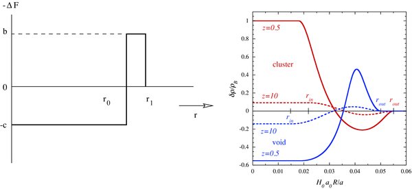
In what follows, we derive analytic formulae for computing temperature fluctuations due to the ISW effect for spherically symmetric compensated top-hat-type density perturbations using the first and second-order perturbation theory (Tomita & Inoue 2008, abbreviated as TI hereafter). The relation between density perturbations of the growing mode and the potential function F of spatial variables are given in Equations (3.6) and (3.11) of TI. The top-hat-type density profile is parameterized in terms of two constants b and c, representing first order density contrasts at the center and at the wall at the present time (Figure A1).
Figure A1. Left: matter density contrast (at linear order) for a top-hat-type spherical void used in our perturbative analysis. Right: density profiles δm in our LTB models as a function of physical radius in units of present Hubble radius for a compensated cluster and void. The initial condition is set at redshift z = 10. We assume a concordant FRW cosmology with (Ωm,0, ΩΛ,0) = (0.26, 0.74) as the background spacetime.
Download figure:
Standard image High-resolution image
The first-order density contrast δL m at a conformal time η when the scale factor is equal to a(η) can be written in terms of the background matter density ρB and the growth function P(η) corresponding to the growing mode of density perturbation as
for (r < r0, r0 < r < r1), respectively, where a prime denotes a partial derivative with respect to conformal time η.
The second-order density contrast is expressed as
for (r < r0, r0 < r < r1), respectively, where ζ1 and ζ2 are given in Equation (2.19) of TI. Here we have omitted the terms that are negligible if r1 ≪ H−1 because we assume that typical size of super-structures is O(100) h−1 Mpc. Neglecting the terms higher than second-order, the total density contrast δρ/ρB can be written as
For a central value of total density contrast, (δρ/ρ)c , we have the relation

where z is the redshift, ![$\alpha (z) \equiv {2\over 3}(\zeta _1 -{9\over 2}\zeta _2)/(\rho _B a^2) - [\beta (z)]^2, \ \beta (z) \equiv ({a^{\prime }\over a}p^{\prime } -1)/(\rho _B a^2)$](https://content.cld.iop.org/journals/0004-637X/724/1/12/revision3/apj368669ieqn9.gif) and γ(z) ≡ 1 − 1/[1 + (δρ/ρ)c
].
and γ(z) ≡ 1 − 1/[1 + (δρ/ρ)c
].
In the text we consider models of supervoids and superclusters with a given set of r0, r1 and (δρ/ρ)c (zc ), where (δρ/ρ)c (zc ) is (δρ/ρ)c at the epoch of redshift zc . From this set we obtain c and b, solving the above equation as

and b is related to c as b/c = 1/[(r1/r0)3 − 1] for compensated super-structures.
The first and second-order temperature fluctuations ΔT(1)/T and ΔT(2)/T are defined by Equations (4.2) and (4.4) of TI. Their expressions for a light path passing the center of spherical voids and clusters are given in Equations (5.11) and (5.13) of TI. For the other light paths, the first-order temperature fluctuation is derived from Equations (5.8) and (5.9) with Equation (C6) of TI and expressed as
where J(r/r0) is given in Equation (C7) of TI for r ⩽ r0. For r1 > r > r0, we have
where u ≡ r/r0, u1 ≡ r1/r0 and
The second-order temperature fluctuation can be derived from Equations (2.17), (2.18), (4.4), and (4.5) of TI and expressed as
where ∫∞ 0 dλ(F,r )2 and ∫∞ 0 dλΦ0 for r < r0 are given in Equations (C3) and (C4) of TI and the expression of ζ'1 and ζ'2 is shown in Equations (4.6) and (4.7) of TI. For r1 > r > r0, we have
where Ii (i = 1 − 3) are given above and I4 is
When we compare the temperature fluctuations in the perturbative model (in Appendix A) and those in the full nonlinear model (in Appendix B), we should notice the difference of their density profiles, i.e., the top-hat profile (in Appendix A) and the Sakai–Inoue (SI) profile (in Appendix B). For our comparison in this paper, we simulate the top-hat profile to the SI profile by equating the outer boundaries and their zero points as follows. Here we represent the SI profile using the radial coordinate r defined in the perturbative model. In the top-hat profile, the radii in the outer boundary and the zero point are r = r1 and r0, respectively, and in the SI profile the radius in the outer boundary is r = rout and the zero point is r = (rin + rc )/2 approximately, in which rc = (rout + rin)/2. If we equate these outer boundaries and zero points, we obtain

Then for relative widths wth
≡ 1 − r0/r1 and wSI
≡ 1 − rin/rout, we have a relation  . In the text we show the temperature fluctuations in both models with parameters which satisfy this relation.
APPENDIX B: METHOD OF COMPUTING REES–SCIAMA EFFECTS USING THE LTB MODELS
Any spherically symmetric spacetime which includes dust of energy density ρ(t, r) and a cosmological constant Λ can be described by the LTB solution,
which satisfies
where ' ≡ ∂/∂r and  .
.
Our model is composed of three regions: an outer flat FRW spacetime, an inner negatively/positively curved FRW spacetime, and an intermediate shell region described by the LTB metric. At the initial time t = ti , which we choose as zi = 10, we define the radial coordinate as R(ti , r) = r, and we assume (Figure A1)
where
Initial velocity field,  , is given by the linear perturbation theory (TI). Then f(r) is determined by Equation (B2). Our model parameters are Ωm,0, rout, w, the redshift of the center of a void/cluster, zc
, and δm
(zc
).
, is given by the linear perturbation theory (TI). Then f(r) is determined by Equation (B2). Our model parameters are Ωm,0, rout, w, the redshift of the center of a void/cluster, zc
, and δm
(zc
).
The wave 4-vector kμ of a photon satisfies the null geodesic equations,
For null trajectories on the θ = π/2 plane, the geodesic Equations (B6) with the metric (B1) reduce to

We use the null condition (B7) not only to set up initial data but also to check numerical precision after time integration.
To integrate the geodesic Equations (B9)–(B11) together with the field Equations (B2) and (B13) numerically, we discretize r into N elements,
and any field variable Φ(t, r) into Φi (t) ≡ Φ(t, ri ). Evolution of Ri (t) is determined by (B2), but we also need data of R'i (t) and R''i (t). Because finite difference approximation, R'i (t) ≈ (Ri + 1 − Ri − 1)/(2Δr), include errors of O(Δr2), we numerically integrate with time,
which is given by differentiating (B2) with respect to r. Furthermore, to vanish R''(t, r) in the geodesic equations, we have introduced an auxiliary variable X. To prepare geometrical values between grid points ri and ri + 1, we adopt cubic interpolation: at each time t* any variable Φ(t*, r) in ri < r < ri + 1 is determined by
We also have to consider null geodesics from an observer to the void/cluster. Suppose that the observer is at the origin and the center of the void/cluster is located at x = xc on the y axis. Then, without loss of generality, on the x–y plane we can analyze light rays which reach the observer. A position on the outer shell and the four momentum of the light there in the observer-centered coordinate are given by

where E is the photon energy and α is the angle between the light ray and the x-axis. Defining l(z) as a comoving length from the observer to the photon, we can write the light path as
The solution of (B15) and (B17) gives
and the null vector in the void/cluster-centered spherical coordinate,
at the time when the photon leaves the shell, zleave.
Our computing algorithm is summarized as follows.
- 1.
- 2.
- 3.
APPENDIX C: TEMPERATURE VARIANCE FOR TOP-HAT COMPENSATING FILTER
In what follows, we derive analytic formulae for computing variance of temperature fluctuations on a sky for a circular top-hat compensating filter Wth (θ; θin). We assume that an ensemble of the CMB fluctuations can be regarded as an isotropic random field on unit sphere S2. Let ΔT(θ, ϕ) be a temperature fluctuation at spherical coordinates (θ, ϕ). Then filterd temperature fluctuation centered at the "north" pole (θ = 0) can be written as
where A = 2π(1 − cos θin). Plugging ΔT expanded in spherical harmonics Ylm ,

into Equation (A1), we have
where
Note that we have used a formula for the Legendre function Pl ,
in deriving Equation (A4). Because ΔT is assumed to be isotropic on S2, the variance of ΔTf can be written as a function of the angular power spectrum Cl as
If the CMB sky is smoothed by a Gaussian beam with the FWHM θs , then the variance is
where Bl = exp [ − σ2 s l(l + 1)/2], and σs = (8ln 2)−1/2θs .
In the absence of complete sky coverage, we cannot directly observe Cl . We can only compute estimated expansion coefficients for the observed region R in the sky (Bunn 1995),
where Nlm is a factor chosen to normalize blm appropriately. If R is azimuthally symmetric, one possible prescription is to set (Peebles 1973)
where
Then a possible estimator for Cl is given by
In the limit that Cl
varies much more slowly than 
we have  .
.