


ABSTRACT
This paper presents a three-dimensional analytical solution, in the limit of very low plasma β-ratio, for the distortion of the interstellar magnetic field surrounding the heliopause. The solution is obtained using a line dipole method that is the integration of point dipole along a semi-infinite line; it represents the magnetic field caused by the presence of the heliopause. The solution allows the variation of the undisturbed magnetic field at any inclination angle. The heliosphere is considered as having blunt-nosed geometry on the upwind side and it asymptotically approaches a cylindrical geometry having an open exit for the continuous outflow of the solar wind on the downwind side. The heliopause is treated as a magnetohydrodynamic tangential discontinuity; the interstellar magnetic field lines at the boundary are tangential to the heliopause. The interstellar magnetic field is substantially distorted due to the presence of the heliopause. The solution shows the draping of the field lines around the heliopause. The magnetic field strength varies substantially near the surface of the heliopause. The effect on the magnetic field due to the presence of the heliopause penetrates very deep into the interstellar space; the depth of penetration is of the same order of magnitude as the scale length of the heliosphere.
Export citation and abstract BibTeX RIS
1. INTRODUCTION
We study the distortion of the interstellar magnetic field surrounding the heliopause from an undisturbed uniform condition at great distances from the heliosphere. The heliopause is treated as a magnetohydrodynamic (MHD) tangential discontinuity; the interstellar magnetic field lines at the boundary are tangential to the heliopause.
In the limit of very low plasma β-ratio, the energy density of the magnetic field is much greater than that of the ionized gases of the interstellar medium; the magnetic field is curl-free everywhere on the interstellar side of the heliopause. There is a well-known analytical solution that describes how the magnetic field on the interstellar side is substantially distorted due to the presence of a spherical heliopause (Parker 1963). The three-dimensional (3D) analytical solution for the magnetic field around a spherical heliopause is the vector sum of the undisturbed magnetic field and a point dipole; the point dipole represents the magnetic field due to the presence of the heliopause (see review articles by Axford 1972; Holzer 1989; Seuss 1990).
Instead of dealing with a spherical heliopause, this research takes into consideration that the heliosphere has blunt-nosed geometry on the upwind side and it asymptotically approaches a cylindrical geometry on the downwind side so that it can have an open exit for the continuous outflow of the solar wind. We obtain an analytical solution by a line dipole method; the line dipole is the integration of point dipole along a semi-infinite line. The line dipole solution represents the magnetic field caused by the presence of the heliopause. The vector sum of the undisturbed interstellar magnetic field and the heliopause field describes the magnetic field on the interstellar side of the heliopause. The undisturbed magnetic field is allowed to have an arbitrary inclination angle with the upwind–downwind line.
The analytical solution is used to construct the geometry of the heliopause and some 3D magnetic field lines on the interstellar side of the heliopause. The interstellar magnetic field is substantially distorted due to the presence of the heliopause. The solution shows the draping of the field lines around the heliopause. The magnetic field strength varies substantially near the surface of the heliopause. The effect on the magnetic field due to the presence of the heliopause penetrates very deep into the interstellar space; the depth of penetration is of the same order of magnitude as the scale length of the heliopause.
2. LINE DIPOLE METHOD
This study chooses the x-axis of a Cartesian coordinates (x, y, z) anti-parallel to the direction of the Sun's motion relative to the interstellar medium; and the x-y plane is parallel to B∞, the undisturbed interstellar magnetic field far from the heliopause; i, j, and k are three unit vectors.
The first step of this study is to consider that the undisturbed interstellar magnetic field B∞ is along the y-direction, namely, B∞ = B∞ j. We choose the origin of the coordinate system at the stagnation point of the heliopause. We may express the analytical solution of Parker (1963) for the distorted magnetic field surrounding a spherical heliopause as the vector sum of the undisturbed interstellar magnetic field B∞ and a point dipole centered at x = a, y = 0, and z = 0
Here,
is the scalar potential, a is the radius of the sphere, B∞a2/2 is the dipole moment, r and λ are related to the Cartesian variables by y = rcos λ and z = rsin λ. The dipole term represents the magnetic field caused by the presence of the heliopause. This solution provides a 3D description for many gross features of the magnetic field on the upwind side of the heliopause. It shows the draping of the field lines around a sphere. And it predicts that at the stagnation point the field strength increases by 50%, i.e., B0/B∞ = 1.5, and the magnetic pressure is significantly enhanced by a factor of 2.25.
We now introduce a line dipole method. A line dipole is the integration of point dipole along a semi-infinite line. We calculate the contribution from the point dipole centered at x = x', y = 0, and z = 0, distributed along x' ⩾ c > 0. We can express the magnetic field of the line dipole as
Here, A and c are constants to be determined, and the point dipole function f is defined in Equation (2). The three components of the line dipole are
The line dipole field F represents the magnetic field caused by the presence of the heliopause; we may call it the heliopause field.
Let us examine the vector sum of the undisturbed interstellar magnetic field B∞ and the heliopause field F

This solution is divergence-free and curl-free; and it reduces to the undisturbed interstellar magnetic field at large distance from the origin. The three components of the field are


We can use this solution to represent the magnetic field on the interstellar side of the heliopause. Making use of the magnetic field equations, Equations (8)–(10), we can calculate 3D numerical solutions for the heliopause and the field lines. The solutions are symmetrical about the x-y plane.
On the surface of the heliopause
This ratio is a function of x and r, and independent of λ. Thus, the shape of the heliopause is symmetrical about the x-axis. We study the numerical solution for the heliopause. We choose that the stagnation point be located at the origin of the coordinate system, and require that the geometry of the heliopause asymptotically approaches a cylinder with radius a at large distances from the stagnation point. The numerical solution of Equation (11), that satisfies the two conditions, determines the two unknown constants

and

Here, the radius a is the scale length of the heliopause.
In Figure 1, we plot the geometry of the heliopause and a few magnetic field lines on x-y plane on the interstellar side of the heliopause. The interstellar magnetic field is substantially distorted near the heliopause. Outside of the x-y plane all field lines have 3D configuration. Some sample field lines on the surface of the heliopause are plotted in Figure 2. They show the draping of the field lines over the interstellar side of the blunt-nosed heliopause.

Figure 1. Geometry of the heliopause and field lines surrounding the heliopause on the x-y plane for χ = 90°. The heliopause is symmetrical about the x-axis; stagnation point is at the origin of the coordinate system; and the heliopause asymptotically approaches a cylinder of radius a.
Download figure:
Standard image High-resolution image
Figure 2. Draping of magnetic field lines around the front face of the heliopause.
Download figure:
Standard image High-resolution imageThe magnetic field strength varies substantially near the surface of the heliopause. The front view of the heliopause is a circular area. The field strength is symmetrical about the x-y plane, and about the x-z plane. Figure 3 shows the iso-intensity contour for B/B∞ on the first quadrant of the front view of the interstellar side of the heliopause. B0/B∞ = 1.638 at the stagnation point. The field strength gets stronger at increasing z, and weaker at increasing y.
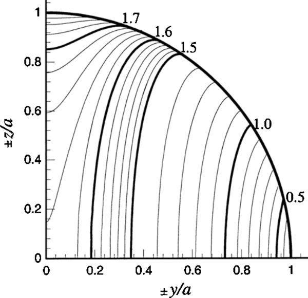
Figure 3. Front view of constant contours of field strength B/B∞ on the surface of the heliopause.
Download figure:
Standard image High-resolution image3. UNDISTURBED FIELD AT AN INCLINATION ANGLE
We continue to study the interstellar magnetic field taking into consideration that the undisturbed field B∞ makes an inclination angle χ with the x-axis at great distance from the heliosphere. Without loss of generality, we can write

We attempt to obtain an analytical expression for the magnetic field surrounding the heliopause in term of dipole solution.
Let us first consider a simple case in which the undisturbed interstellar magnetic field B∞ is parallel to the x-axis B∞ = B∞ i, i.e., the inclination angle χ = 0. In this case, we again choose the origin of the coordinate system at the stagnation point of the heliopause. The field lines and the heliopause are symmetrical about the x-axis; the magnetic field on the interstellar side of the heliopause may be represented by the vector sum of B∞ and a line dipole G

Here, the vector G, that represents the magnetic field caused by the presence of the heliopause, is the integration of the point dipole along a semi-infinite line
The scalar potential g is a point dipole centered at x = x', y = 0, and z = 0
Two non-zero components of G are
When the inclination angle χ = 0, analytical solutions for the heliopause and the field lines can be obtained from
Integration of Equation (20), one can obtain the equation for the heliopause
This equation has often been used to sketch the heliopause geometry (Parker 1963; Holzer 1989; Seuss 1990).
Equations (7) and (15) are analytical solutions for inclination angle χ = 90° and 0°. The solutions are divergent-free and curl-free; they, respectively, reduce to the undisturbed interstellar conditions at large distance from the heliosphere. The stagnation point of the heliopause represented by each solution is at the origin of the coordinate system. The heliopause has a blunt-nosed geometry axisymmetrical about the x-axis; it asymptotically approaches a cylinder at large distances from the stagnation point.
For the general case, that the undisturbed field B∞ makes an inclination angle χ with the x-axis, we may express the solution for the distorted magnetic field surrounding the heliopause as a linear combination of the two dipole solutions, Equations (7) and (15),

The two vectors F and G are given in Equations (3) and (16); Fsin χ + Gcos χ represents the magnetic field caused by the presence of the heliopause. The magnetic field is the vector sum of the undisturbed interstellar magnetic field and the heliopause field. The vector sum remains divergent-free and curl-free. Three components of the magnetic field are


We have calculated the magnetic field as the vector sum of the undisturbed interstellar magnetic field and the heliopause magnetic field. In Figure 4, we plot the geometry of the heliopause and some field lines on the x-y plane for χ = 30° and 60°. The inclination angle produces departure of the heliopause geometry from axial symmetry about the x-axis. Lallement et al. (2005) reported that the direction of the neutral hydrogen flow in the heliosphere is deflected relative to the helium flow by about 4°, caused by a distortion of the heliosphere under the action of an inclined interstellar magnetic field.
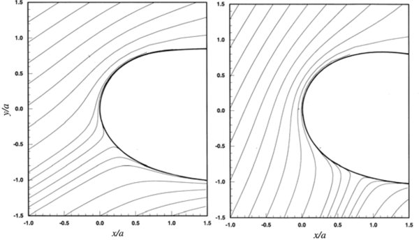
Figure 4. Geometry of the heliopause and field lines surrounding the heliopause on the x-y plane for χ = 30° (left panel) and χ = 60° (right panel).
Download figure:
Standard image High-resolution imageThe magnetic field lines and the heliopause are symmetrical about the x-y plane. The magnetic pressure B28πon the interstellar side plays an important role in dynamical balance between two sides of the heliopause. The ratio B2/B2∞ measures the variation of the magnetic pressure. From Figure 3, we can visualize that the magnetic pressure would change substantially over the surface of the heliopause.
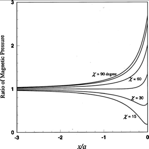
In Figure 5, we plot the magnetic pressure ratio B2/B2∞ along the x-axis. It shows that the inclination angle has a significant effect on the magnetic pressure near the heliopause. If we define the enhancement factor as the magnetic pressure ratio at the stagnation point, B20/B2∞, then the enhancement factor varies significantly with the inclination angle, its maximum value is B20/B2∞ = 2.68 at χ = 90°. From Figure 5, we also see that the effect on the magnetic field due to the presence of the heliopause penetrates very deep into the interstellar space; the depth of penetration is of the same order as the dimension of the heliopause.
Figure 5. Magnetic pressure ratioB2/B2∞along the x-axis at varying inclination angle χ.
Download figure:
Standard image High-resolution image
4. DISCUSSION
4.1. Image Dipole Method
In this study, we use dipole solutions to represent the magnetic field due to the presence of the heliopause. This method is known as the image dipole method in studying the planetary magnetospheric magnetic field. Chapman & Ferraro (1931) first used an image dipole of moment equal to the earth's dipole to simulate the distortion of the Earth's magnetic field. Hones (1963) and Taylor & Hones (1965) used an image dipole of strength greater than earth's to obtain a model in which the earth's field distorted by the solar wind is confined inside the magnetopause. The image dipole method has also been used in studying the magnetosphere of Mercury (Whang 1977). In these studies, point dipoles were used to represent the magnetic field caused by the presence of the planetary magnetopause.
This research studies the integration of point dipole along a semi-infinite line; it demonstrates that, in the limit of very low plasma β-ratio, the line dipole can be used to represent the substantial distortion of the magnetic field vector on the interstellar side of the heliopause.
4.2. Plasma β-ratio
We now try to calculate the range of possible value of the plasma β-ratio for the interstellar medium. The plasma beta is a function of the proton number density N, the temperature T, and the magnetic field intensity B∞. In various model studies, the frequently used numbers are N = 0.07–0.1 cm−3, T = 7000–10,000 K, and B∞ = 2–5 μG. We also take into account additional numbers reported by researchers. (1) Using measurements performed inside the heliosphere and inferred from analysis based on numerical modeling, Izmodenov (2009) estimated that the interstellar proton number density N = 0.05 ± 0.015 cm−3. (2) Based on analysis of measurement made along the Ulysses orbit, Witte (2004) reported that the interstellar helium has a temperature of T = 6300 ± 340 K. (3) Cox & Helenius (2003) have a model to study the formation of the Local Cloud; the model predicted that the interstellar magnetic field has "a field strength of about 6 or 7 μG".
Using N = 0.035–0.1 cm−3 and T = 6000–10,000 K, we calculate the β-ratio for B∞ to vary from 2 to 7 μG as shown in Table 1. The result shows that the plasma β-ratio can be much less than 1 in the interstellar medium.
Table 1. Plasma β-ratio, Alfven Speed, and Magnetosonic Speed as Functions of the Field Magnitude B∞ for Proton Number Density N = 0.035–0.1 cm−3 and Plasma Temperature T = 6000–10,000 K
| B∞ (μG) | β-ratio | Alfven Speed (km s−1) | Magnetosonic Speed (km s−1) |
|---|---|---|---|
| 2 | 0.36–1.73 | 13.8–23.3 | 18.9–28.6 |
| 3 | 0.16–0.77 | 20.7–35.0 | 24.4–38.7 |
| 4 | 0.09–0.43 | 27.6–46.6 | 30.4–49.5 |
| 5 | 0.06–0.28 | 34.5–58.3 | 36.8–60.6 |
| 6 | 0.04–0.19 | 41.4–70.0 | 43.3–71.9 |
| 7 | 0.03–0.14 | 48.3–81.6 | 50.0–83.3 |
Download table as: ASCIITypeset image
We have also calculated, in Table 1, the Alfven speed, and the magnetosonic speed Cf = (c2 + a2)1/2, where c is the gasdynamic sound speed and a is the Alfven speed. If the interstellar field B∞ is less than ∼3 μG, the flow speed V can be greater than the magnetosonic speed, and a bow shock should appear on the upstream side of the heliopause. MHD models have been used by many authors to study the interaction between the interstellar medium and the heliosphere (Baranov & Zaitev 1995; Florinski et al. 2004; Linde et al. 1998; Neutsch & Fahr 1982; Opher et al. 2004, 2006; Pogorelov et al. 2004, 2006; Ratkiewicz et al. 1998; Tanaka & Washimi 1999; Washimi & Tanaka 1996). In this case, the distortion of the interstellar magnetic field is confined in the narrow region between the bow shock and the heliosheath. However, if the interstellar field B∞ is stronger, the flow speed V becomes less than the magnetosonic speed, no bow shock should occur upstream of the heliopause. In this case, the result of this research shows that the effect on the magnetic field due to the presence of the heliopause penetrates very deep into the interstellar space; the depth of penetration is of the same order of magnitude as the scale length of the heliopause.