


ABSTRACT
We present estimates of Vega's composition, mass, and age based on a simultaneous fit of high-resolution metal line profiles, the wings of the Balmer lines, the absolute visible/near-IR fluxes, and high angular resolution triple phase data from the Navy Prototype Optical Interferometer to gravity-darkened Roche models. This substantially expands our earlier analysis. We determine that Vega has a much lower mass, 2.135 ± 0.074 M☉, than generally assumed. This strongly supports the contention that Vega is metal-poor throughout (Z ∼ 0.008), suggesting it was formed that way. Assuming a uniform composition equal to that derived for the surface, and the luminosity and radius obtained here, we derive a best estimate of Vega's age, 455 ± 13 Myr, and mass, 2.157 ± 0.017 M☉, by fitting to standard isochrones. We continue to argue that Vega is much too old to be coeval with other members of the Castor moving group and is thus unlikely to be a member. The updated chemical abundances continue to support the conclusion that Vega is a λ Boo star.
Export citation and abstract BibTeX RIS
1. INTRODUCTION
Vega (α Lyr, HR 7001, HD 172167) is a sharp-lined, Population I star of spectral type A0Va (Gray & Garrison 1987) with a projected rotational velocity of 22 km s-1 (Gulliver et al. 1994). It has taken the role of the primary absolute photometric standard in the visual (Hayes 1985) due to its apparent brightness and convenient access from northern observatories. Recent studies have found a somewhat low metallicity (Sadakane & Nishimura 1981; Adelman & Gulliver 1990) even while it served as a comparison star for abundance studies (e.g., Venn & Lambert 1990). Since the similarity between its abundance pattern and those of the λ Boo stars was noticed (Baschek & Slettebak 1988), it has been debated whether Vega should be included among this group (Ilijić et al. 1998). A recent kinematics study has also identified Vega as a member of the Castor moving group, whose age has been estimated as 200 ± 100 Myr using kinematics, isochrones, and lithium abundances (Barrado y Navascués 1998).
Gray (1988) was the first to note that Vega's apparently excessive luminosity (Petrie 1964) could be explained if it were rapidly rotating and nearly pole-on. This was followed by the discovery that high signal-to-noise ratio (S/N), high-resolution spectra (Gulliver et al. 1994) showed Vega's weak lines to have a flat bottom appearance, which also had an explanation in strongly projected rotation. Initial estimates of the equatorial velocity, veq ∼ 245 km s-1 (Gulliver et al. 1994), were subsequently revised downward to veq ∼ 175 km s-1 (Hill et al. 2004), a result which gained support from the extensive spectroscopic study of Takeda et al. (2008).
In the meantime, advances in long baseline optical interferometry saw the opening of instruments such as the Navy Prototype Optical Interferometer (NPOI; Armstrong et al. 1998) and the Center for High Angular Resolution Astronomy array (CHARA; ten Brummelaar et al. 2005) which were able to resolve Vega's disk. This lead quickly to the announcement that the surface brightness distribution in the visible (Peterson et al. 2004, 2006, hereafter P06) and near-IR (Aufdenberg et al. 2006) indicated Vega was indeed pole-on (i ∼ 5°), rotating at ∼90% of breakup (veq ∼ 275 km s-1).
These high velocities result in large temperature gradients (∼2000 K) across the visible disk, raising questions about the adequacy of previous abundance studies, and the accuracy of the other inferred physical properties. This led (Yoon et al. 2008, hereafter, Y08), using spectra from the ELODIE archive (Moultaka et al. 2004), to reanalyze the spectrum. In the process, they pointed out that the peculiar shapes of the weak lines are strongly correlated with excitation and ionization potential and can be understood in terms of how the Boltzmann factors amplify the temperature gradient across the disk. Since Vega is seen nearly pole-on, the center of the apparent disk is almost exactly at one pole, the hottest point on the star. In addition, they found that good quantitative fits to the line profiles required introducing macroturbulence. The resulting abundances reinforced the identification of Vega as a λ Boo object. It was pointed out that if Vega was well mixed, presumably through meridional currents, then it was significantly less massive (∼2.1 M☉) and older (∼540 Myr) than previously estimated (e.g., Song et al. 2001).
The lack of consistency among the various methods used to determine the equatorial rotation velocity of Vega is problematic. The purely spectroscopic studies (Gulliver et al. 1994; Takeda et al. 2008) derive relatively low velocities (ω ≈ 0.7, where ω is the angular velocity as a fraction of breakup), whereas the interferometric determinations (P06; Aufdenberg et al. 2006) settle above ω = 0.9. Y08 proposed that the muted line profile features, which led to the low spectroscopic rotation rates, were the result of extensive macroturbulence which would be consistent with rapid rotation. That this is the correct explanation is important to verify. In pole-on cases like Vega, it is much easier to determine the effect that rotation has on the limb darkening through visibility amplitude measurements (e.g., Aufdenberg et al. 2006), than through the relatively small changes in the visibility phases (e.g., P06). However, if one cannot rely on the line profiles being simply related to the effects of projection, then the comparison of the apparent velocity widths with the interferometrically determined absolute rotation rate cannot be relied on to determine the inclination. Unfortunately, we do not at the moment see a way to independently check whether macroturbulence is present in the amounts derived by Y08 for Vega, and will not consider the matter further here.
The other major question raised by Y08, alluded to above, involves the bulk composition of Vega. Is the very unusual surface composition representative of the entire envelope, and possibly the whole star initially, or is it just another example of the kinds of outer envelope effects exhibited by the Am and Ap objects and their hotter and cooler relatives, with the basic solar composition better reflecting the composition of the interior? Y08 argue that the latter is extremely unlikely because of Vega's very high inferred rotation. But modern investigations of angular momentum transport in the envelopes of rotating stars (e.g., Zahn 2008) paint a very complicated picture of the circulation currents that are usually identified as the main source of mixing.
There is a way of getting the beginnings of an answer to this last question. Solar composition stars have very different values of luminosity, radius and mass than stars would have with the bulk composition equal to the abundances derived in Y08, even allowing an unknown amount of evolution. To this end, we consider here a fully self-consistent calculation of a rotating model of Vega incorporating the original NPOI observations, the absolute calibration of Vega in the visible, the Balmer line profiles, and a selection of isolated, low excitation, metal line profiles, in a simultaneous reduction to identify the optimal parameters for the star, including an ab initio estimate of its mass. With these results, we will show that it is very likely that Vega is chemically homogeneous over the bulk of its interior. It is likely that this was its initial state.
This paper proceeds as follows. The observational data are described in the following section, and the Roche modeling is briefly summarized in Section 3. In Section 4, we describe how we model the observables: the continuum flux, the hydrogen Balmer lines, the line profiles of Ca i λ 6162 and Mg i λ 4702, and the interferometric observables. ATLAS12 (Kurucz 2005) model atmospheres specifically calculated for Vega are used throughout. We next discuss the model fitting, compare our results with the previous studies, note the abundance changes due to the new models, and determine the best estimate of Vega's metallicity, mass, and age and discuss its significance. The summary follows in Section 6.
2. THE OBSERVATIONAL DATA
The interferometric data were taken by the NPOI on 2001 May 25 in the visible (P06). We focus here on the triple phase data taken that night. Triple phases are obtained by summing the calculated phases for the three baselines (AW–AE–W7 in this case), with due attention to tracing around the triangle properly and are very sensitive to asymmetries in the intensity distribution, as described by P06 where details of the observations and data reduction are given.
In addition to the interferometry, we include a number of other observables necessary to complete the modeling as described in P06. In the process, a number of refinements have been made. We will use the absolute visible fluxes (Hayes 1985) rather than just the V magnitude. There are two reasons for this. First, no absolute calibration has ever been done using broadband filters. As a result, one must adopt filter transmission curves and determine scaling factors in order to predict the observed magnitudes from theoretical models, a process that introduces its own set of errors. Second, since the visible calibration covers a range of wavelengths, the flux gradient provides an important constraint in the modeling, independent of the zero point. We chose to limit our use of published absolute calibrations of Vega to the near-UV/visible/red region because they are "mature" in the sense described by Hayes (1985). These data are not rigorously statistically independent, point-to-point, and to prevent the large number of data points from being given undue weight in the reductions we used only every fourth point as tabulated by Hayes (1985). In addition, we excluded the fluxes in the spectral regions affected by hydrogen lines or strongly contaminated by telluric lines. We adopt a 1% estimate of the uncertainty longward of the Balmer discontinuity as suggested by Hayes, but increase that to 3% in the Balmer continuum, based on the divergence of the various determinations there. In the end, we have used 30 calibration points from the Hayes (1985) tables over the range 3300 Å to 8000 Å.
In choosing which photometric data to model, we have been particularly conservative. For example, the Oxford Group (e.g., Mountain et al. 1985, and references therein) has made a number of calibrated measurements in the near-IR. However, the data have fairly large uncertainties and would provide no effective constraints, nor have they been repeated by other groups and hence are not "mature" in Hayes' sense. For the UV, Bohlin & Gilliland (2004) have proposed a calibration based on model atmosphere fits to White Dwarfs. While we know of no reason this should not work and suspect that it would provide some constraints (e.g., Aufdenberg et al. 2006), we nevertheless decided to rely exclusively on the primary measurements described above.
We also add the profiles of the three lowest Balmer lines, Hα, Hβ, and Hγ, as given by Peterson (1969). These features are sensitive to surface gravity and hence provide an estimate of the mass. Comparison with more recent measurements (Gray & Evans 1973; Adelman & Gulliver 1990) indicate that these are reliable measurements and if anything, the published uncertainties (1%) are overly conservative.
The Vega spectra used here are from the ELODIE archive, which contains resolution ∼42, 000 echelle spectra from the ELODIE spectrograph obtained at the Observatoire de Haute-Provence 1.93 m telescope. The details of how the ELODIE spectra were co-added are given in Y08. For model fitting of individual spectral lines, Ca i λ 6162 and Mg i λ 4702 were used because those have low excitation potentials thus show clearly the double-horned shapes, are relatively free of blends, have a clean continuum, and a good S/N. We also consider the profiles of O i λ 6155 and Fe ii λ 4522, higher excitation lines, which are stronger lines but are otherwise free from obvious blends and other problems.
3. MODELING
We model Vega as a rapidly rotating star using a gravity-darkened Roche spheroid in solid-body rotation with a point mass gravitational potential, which induces a temperature gradient (Teff(θ) ∝ g0.25eff(θ) where θ is the co-latitude) over the surface (von Zeipel 1924). Since intermediate-mass stars have radiative envelopes and relatively small convective cores, solid-body rotation appears to be a good approximation for the external layers of early-type stars (Spiegel & Zahn 1992; Reiners & Royer 2004).
Roche modeling for isolated rotating early-type stars is described in P06, but a brief description is useful here. This model requires six parameters to describe the star, including the inclination angle, i, the position angle, P.A., the surface gravity at the pole, gp (or, equivalently the mass, M), the polar angular diameter, θp (or equivalently the radius, R, through the parallax, p), the polar effective temperature, Tp, and the fractional angular velocity, ω. With these parameters, we calculated the specific intensity over the surface assuming that LTE, hydrostatic equilibrium, and plane-parallel atmospheres apply locally.
One more parameter, the macroturbulent velocity, VMac, must be added to complete the specification of our model. Macroturbulence was found by Y08 to be needed to match the observed line profiles. If substantial broadening of this type is present generally in rapidly rotating stars, Vega is one of the few stars with sharp enough lines where its effects might be detected. The theory of macroturbulence is not well developed, so two simple approximations are considered here: isotropic macroturbulence and horizontal (velocities are perpendicular to the local normal) macroturbulence. In the latter case, the projected velocity dispersion has a view-angle dependence given by

where VMac is the fitted constant and μ is the cosine of the angle between the line of sight and the local normal. In this case, the broadening is maximum at the limb and vanishes toward the center of the disk.
In practice, we look at a point on the surface and calculate the line-of-sight dispersion the turbulence model provides, then calculate the line profile and store it. We do this for each patch and then co-add all the line profiles, properly intensity weighted, to yield the emergent flux profile. Broadening by macroturbulence does not change the total absorption (equivalent width) of the spectral lines locally, unlike microturbulence (Gray 2005).
4. COMPUTATIONS
To determine the parameters of the Roche model, several observables need to be calculated. These include the absolute flux over the near-UV/visible/red spectrum which provides information about the temperature and angular diameter, the Balmer line profiles, which constrain Tp and gp, the spectral line profiles of the Ca i and Mg i lines to obtain the projected equatorial velocity, veqsin i, and VMac, and the NPOI triple phases which are sensitive to the fractional angular rotational velocity, inclination angle, position angle, and angular diameter.
The model parameters are fitted by minimizing the χ2 metric utilizing the Levenberg–Marquardt algorithm (L–M; Press et al. 1992). Details of how the spectroscopic and interferometric observables were calculated, follow.
4.1. Spectral Synthesis Method
As described in Y08, the synthetic spectrum was calculated by integrating the emergent flux over the apparent stellar disk. The projected disk is constructed inside a square 256 × 256 grid. The stellar parameters were obtained at the center of each pixel containing part of the flattened disk, and the specific intensity for each cell as a function of λ was computed along with the projected velocity. A grid of 116 ATLAS12 models and spectra were adopted that span the range of effective temperature and surface gravity, assuming a 2 km s-1 microturbulence, specifically calculated for this purpose using the abundance given in Y08, providing specific intensities tabulated at 17 values of μ. The intensity spectra were interpolated in effective temperature, surface gravity, and μ for each cell. The atomic line data were taken from the extensive compilation of Kurucz & Bell (1995). We adopted 2 km s-1 for the microturbulence as described in Y08.
4.2. Spectral Energy Distribution
Based on the synthetic spectra described above, the spectral energy distribution was calculated in the spectral bands of the subset of measured fluxes we have selected from the Hayes (1985) compilation. Boxcar averages of the fluxes over 25 Å wide segments centered on the selected wavelengths were computed. Here the Doppler shift due to projected rotational velocity at each cell is not considered because of the low resolution. This theoretical spectral energy distribution is compared with the observed spectrophotometric data (Hayes 1985) as described in Section 2.
4.3. Hydrogen Balmer Lines Hα, Hβ, and Hγ
We adopt the same procedure in calculating the synthetic hydrogen line profiles as used by Peterson (1969). That is, we limited our calculations to 160 Å segments centered on the lines and chose the regions at 70 Å from the line center to define the continuum. In this case, the Doppler smearing due to rotation is included. Emergent fluxes at symmetric wavelengths on both sides of the line centers were averaged to produce the predicted line profiles. For Hα, the observed point nearest the line core is excluded because the LTE models do not predict the core of this line very accurately.
4.4. Spectral Lines: Ca i λ 6161 and Mg i λ 4702
The lines of Ca i λ 6162 and Mg i λ 4702 were synthesized with a sampling of λ/Δλ = 500, 000 usually used in ATLAS, then convolved down to R = 42,000 using a Gaussian, which is the ELODIE spectrograph resolution. At projected velocities near 20 km s−1, rotational smearing clearly dominates the line profiles.
There are two complications in fitting these spectral lines. First, it is necessary to add additional broadening to the synthetic lines to allow for the effects of macroturbulence. Macroturbulent broadening was introduced in the fitting process by linearly interpolating among line profiles calculated at five different resolutions: R = 20,000, 25,000, 30,000, 38,000, and 42,000. In each case, the convolving profiles were Gaussian, corresponding to turbulent velocities of 13.18, 9.64, 6.99, 3.36, and 0.00 km s-1 .
The other complication is that we must match the line strengths of the synthetic lines to that of the observed lines. Rotation affects the equivalent widths of the lines (Y08) and thus the strengths of the computed lines must be adjusted (i.e., a new abundance estimated) at each iteration of the fitting. In this regard, Ca i λ 6162, a weak line on the linear part of the curve of growth, can be fitted more easily than an intermediate strength line such as Mg i λ 4702. The residual flux of a weak line can be adjusted to match the observed line by simply scaling the line depth with the ratio of the equivalent width of the synthetic line to that of the observed line. The scaled residual flux, R'λ, is given by
where Rλ is the residual flux calculated at given parameters before scaling and Ws and Wo are the equivalent widths of the synthetic line and the observed line, respectively.
Mg i needs to be treated more carefully. Several line profiles at different abundances which bracket the required line strength were pretabulated with the ATLAS12 grid. At each iteration, a chi-squared quantity is then calculated by comparing the observed and synthetic fluxes produced for the different abundances. By parabolic interpolation we obtained the χ2 minimum, and in turn the corresponding abundance. We then calculate the line profile by simple linear interpolation.
Since the metal line profiles contain both shape and width information, we have removed the veqsin i constraint from the model fitting process, which had been imposed by P06.
4.5. Complex Visibility Calculation
The interferometric observables are the amplitude and phase of the complex visibility which is proportional to the Fourier transform of the intensity distribution on the object (the van Cittert–Zernike Theorem; e.g., Thompson et al. 1994, p. 73). The intensities are computed using the detailed limb angle dependence provided by the ATLAS12 model atmospheres. As mentioned, we use only the triple phase data.
5. DISCUSSION
5.1. Model Fitting
The best-fitting model parameters are ω = 0.8760 ± 0.0057, θp = 2.8332 ± 0.0078 mas, Tp = 10059 ± 13 K, i = 4 975 ± 0081, P.A. = 114 ± 21, M = 2.135 ± 0.075 M☉, and VMac = 7.65 ± 0.45 km s-1 using the isotropic model for the macroturbulence. These and various derived parameters are summarized in Table 1, while the correlation matrix for this case is given in Table 2.
Both macroturbulence models match the line profiles well. The plots of the (best-fitting) isotropic macroturbulence model for the continuum flux, Balmer lines, spectral lines, and triple phases are shown in Figures 1, 2, 3, 4, 5, 6, and 7, respectively. The fits based on the horizontal macroturbulence also summarized in Table 1 are indistinguishable from the isotropic case and we show only the latter. One sees excellent fits of the model to the observations, as evidenced by both the plots and χ2. We also tabulate how much each type of data contributes to the χ2 in Table 3.

Figure 1. Shown is the energy distribution in the visual/red for the isotropic macroturbulence case. The open circles represent the absolute calibration given by Hayes (1985), error bars are also shown (1% error in the visual and 3% error in the Balmer continuum). The points represent the calculated values. Residuals from the fit are shown below. The model fits the observed fluxes extremely well, not only in terms of the zero point but also without a noticeable trend in the residuals.
Download figure:
Standard image High-resolution image
Figure 2. Shown is the model fit to the Hγ line profile. Symbols are as in Figure 1. The observations are taken from Peterson (1969) where the errors were estimated at 0.01 in residual intensity. The hydrogen Balmer lines depend somewhat on temperature but mostly constrain the surface gravity, allowing a direct estimate of mass.
Download figure:
Standard image High-resolution image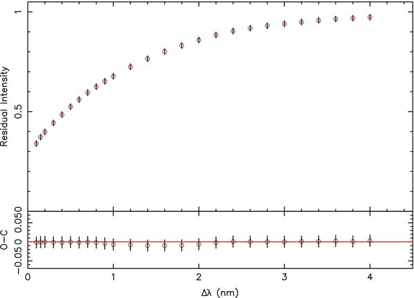
Figure 3. Hβ line profile plotted as in Figure 2. The observational error was estimated to be 0.015 in residual intensity.
Download figure:
Standard image High-resolution image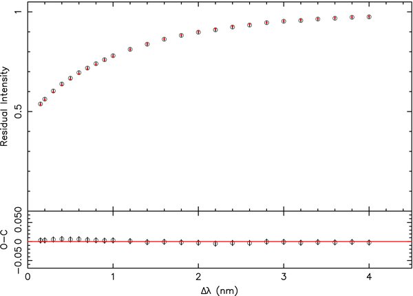
Figure 4. Hα line profile, plotted as in Figure 2. Errors here were estimated to be 0.007 in residual intensity.
Download figure:
Standard image High-resolution image
Figure 5. Shown is the line profile fit to a weak Ca i line (λ 6162). The synthetic spectrum fits the observed profile very well. The self-reversed shape of this low excitation line constrains the macroturbulent velocity.
Download figure:
Standard image High-resolution image
Figure 6. Model fit to an intermediate strength line profile of Mg i (λ 4702). This fit, which is very good, is consistent with that for the weak Ca i (λ 6162) line.
Download figure:
Standard image High-resolution image
Download figure:
Standard image High-resolution image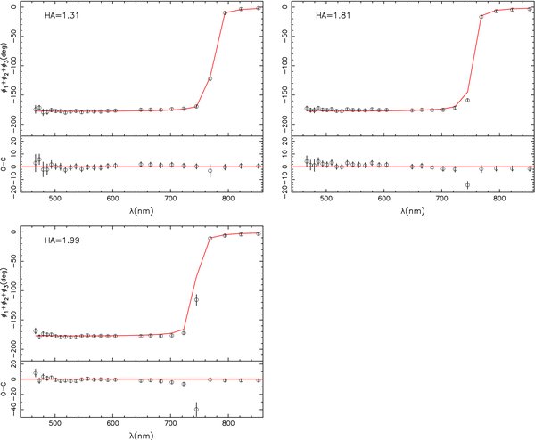
Figure 7. NPOI triple phase (ϕ1 + ϕ2 + ϕ3) observations (open circles), estimated error bars, and the model calculations (solid lines) are plotted as a function of hour angle. Residuals are shown directly below each of the scans. If an object is centrosymmetric, the triple phases take on only 0° or 180° (called as "top-hat" behavior). Significant departures from this simple top-hat behavior are due to asymmetry in the surface intensity distribution. The phases measured here clearly indicate that Vega's intensity distribution is asymmetric.
Download figure:
Standard image High-resolution image
Table 1. Best-Fit Parameters for Vega
| Quantitya | Isotropic VMacb | Horizontal VMacb |
|---|---|---|
| Model Parameters | ||
| ω = Ω/ΩB | 0.8760 ± 0.0057 | 0.8713 ± 0.0035 |
| θp (mas) | 2.8332 ± 0.0078 | 2.8396 ± 0.0048 |
| Tp (K) | 10059 ± 13 | 10049.1 ± 8.2 |
| i (°) | 4.975 ± 0.081 | 5.066 ± 0.077 |
| P.A. (°) | 11.4 ± 2.1 | 11.27 ± 2.0 |
| M (M☉) | 2.135 ± 0.074 | 2.165 ± 0.075 |
| VMac (km s-1) | 7.65 ± 0.45 | 8.75 ± 0.56 |
| Derived Parameters | ||
| veq (km s-1) | 236.19 ± 3.65 | 235.52 ± 3.52 |
| veq,B (km s-1) | 338.99 ± 5.62 | 340.98 ± 5.78 |
| veqsin i (km s-1) | 20.48 ± 0.11 | 20.80 ± 0.11 |
| Ω (d−1) | 1.656 ± 0.023 | 1.653 ± 0.026 |
| ΩB(d−1) | 1.891 ± 0.032 | 1.897 ± 0.033 |
| Teq(K) | 8152 ± 42 | 8184 ± 27 |
| Rp (R☉) | 2.362 ± 0.012 | 2.367 ± 0.011 |
| Req (R☉) | 2.818 ± 0.013 | 2.815 ± 0.012 |
| θmin (mas) | 3.3753 ± 0.0049 | 3.3716 ± 0.0029 |
| θmax (mas) | 3.3802 ± 0.0050 | 3.3766 ± 0.0030 |
| log L (L☉) | 1.6034 ± 0.0049 | 1.6058 ± 0.0044 |
| log gp (cm2 s−2) | 4.021 ± 0.014 | 4.025 ± 0.015 |
| log geq (cm2 s−2) | 3.655 ± 0.021 | 3.668 ± 0.018 |
| Age (Myr) | 471 ± 57 | 449 ± 57 |
| Z | 0.0080 ± 0.0033 | 0.0093 ± 0.0033 |
| Number of data | 334 | 334 |
| χ2 | 223.89 | 224.64 |
Notes. aSymbols not defined in the text are: veq,B (break-up equatorial velocity), Ω (angular velocity), ΩB (break-up angular velocity), Teq (effective temperature at the equator), Req (equatorial radius), θmin,max (minimum and maximum projected angular diameters), L (luminosity), gp (surface gravity at the pole), and geq (surface gravity at the equator). bThe parallax error is included in the error estimates.
Download table as: ASCIITypeset image
Table 2. Correlation Matrix for the Isotropic Macroturbulence Case
| Parameter | i | ω | θp | P.A. | Tp | M | VMac |
|---|---|---|---|---|---|---|---|
| i | 1.0000 | −0.3032 | 0.3297 | −0.2205 | −0.5506 | −0.6283 | −0.1075 |
| ω | −0.3032 | 1.0000 | −0.9932 | −0.3141 | 0.8461 | −0.5015 | 0.1400 |
| θp | 0.3297 | −0.9932 | 1.0000 | 0.3268 | −0.8682 | 0.4746 | −0.1345 |
| P.A. | −0.2205 | −0.3141 | 0.3268 | 1.0000 | −0.1769 | 0.4300 | −0.0152 |
| Tp | −0.5506 | 0.8461 | −0.8682 | −0.1769 | 1.0000 | −0.1752 | 0.0779 |
| M | −0.6283 | −0.5015 | 0.4746 | 0.4300 | −0.1752 | 1.0000 | −0.0986 |
| VMac | −0.1075 | 0.1400 | −0.1345 | −0.0152 | 0.0779 | −0.0986 | 1.0000 |
Download table as: ASCIITypeset image
Table 3. Individual χ2's for the Isotropic Macroturbulence Case
| Data | N.Obs.a | χ2 | References |
|---|---|---|---|
| Visible flux | 30 | 12.44 | Hayes (1985) |
| Hγ | 26 | 1.05 | Peterson (1969) |
| Hβ | 26 | 2.13 | Peterson (1969) |
| Hα | 25 | 6.15 | Peterson (1969) |
| Ca i λ 6162 | 24 | 5.15 | ELODIE |
| Mg i λ 4702 | 21 | 5.98 | ELODIE |
| Triple phase | 182 | 191.00 | P06 |
| Total | 334 | 223.89 | ... |
Note. aNumber of observed data points.
Download table as: ASCIITypeset image
5.2. Fitting Strong Lines
In the process of selecting lines to include in the final fitting, we also considered lines with higher excitation/ionization energies, that is lines which are contributed more from the hotter polar regions. As with the low excitation lines, practical considerations lead to selecting an Fe ii line (4522 Å) and an O i triplet (6155 Å) for analysis. Both these lines are significantly stronger than the low excitation lines described earlier.
When we added the high excitation lines to the reduction, both the isotropic and the horizontal macroturbulence models gave bad fits to the profiles with the isotropic model being slightly preferred. There was a clear conflict when attempting to simultaneously fit the weak and strong lines. The weak lines tend to require a higher temperature and faster rotation, while the strong lines tend to be cooler (Tp ∼ 10, 013 K) and slower (ω ≈ 0.84) model. Because they should be less dependent on any inadequacies in the model atmospheres, we decided to use only the weak Ca i line and the intermediate strength Mg i line in the final fits. The reasons for the inconsistency between the two sets of lines are not clear at present. One possibility is that the assumption of solid-body rotation might need to be relaxed. However, we do not know what kind of figure the differential rotation would produce, so we leave this as an intriguing issue to be resolved in the future.
5.3. Comparison with Previous Studies
It is not straightforward to compare our results with those previously reported since the individual studies used different data sources (Dominion Astrophysical Observatory: Gulliver et al. 1994; Hill et al. 2004; Okayama Astrophysical Observatory: Takeda et al. 2008; ELODIE archive, and so on) and techniques (interferometry or spectroscopy). For example, the CHARA study (Aufdenberg et al. 2006) used visibility amplitude data and spectrophotometry extending from the UV into the IR but did not fit the Balmer lines nor metal line profiles (instead simply adopting a mass, M = 2.3 M☉, and a projected velocity). The NPOI interferometry (P06) used only triple phase data with V magnitude and veqsin i constraints. In the most recent discussion by Hill et al. (2004), there were some problems with the calculation as reported in Aufdenberg et al. (2006), although another recent spectroscopic study (Takeda et al. 2008) supports the parameters reported there.
However, some qualitative comparisons can be made. The situation is summarized in Table 4. The spectroscopic studies show significantly slower rotation than found here. We focus on the results by Takeda et al. (2008) as typical of the spectroscopic studies. They did not consider the possibility of macroturbulence. As a result, their deduced parameters are at odds with those based on interferometry, leading them to suggest that Aufdenberg et al. (2006) in particular had accepted a false χ2 minimum. These lead us to wonder if we could reproduce the Takeda et al. (2008) results and if so, whether our fitting procedure, starting with the parameters given there, would nevertheless converge to the parameters we report here. For this purpose, the interferometric triple phase data and Balmer line profiles were removed and the constraints of veqsin i = 22 km s-1 and a mass of 2.3 M☉ were added. The results are shown in Table 5. The resulting parameters are somewhat different from Takeda et al.'s (2008) results. Our result (ω ∼ 0.75) for the rotation rate is quite close to theirs (ω ∼ 0.7). Remaining differences are undoubtedly due to the choice of lines (we used only two) and that Takeda et al. (2008) did not attempt to formally optimize their model.
Table 4. Comparison with Previous Results
| Parameter | P2006a | A2006b | TKO2008c | This Work |
|---|---|---|---|---|
| ω = Ω/ΩB | 0.926 ± 0.021 | 0.91 ± 0.03 | 0.703d | 0.876 ±0.006 |
| Rp (R☉) | 2.306 ± 0.031 | 2.26 ± 0.07 | 2.52+0.05−0.07 | 2.36 ± 0.01 |
| Tp (K) | 9988 ± 61 | 10150 ± 100 | 9867+86−79 | 10060 ± 10 |
| i (°) | 4.54 ± 0.33 | 4.7 ±0.3 | 7.2+1.7−1.2 | 4.98 ± 0.08 |
| veq (km s-1) | 274 ± 14 | 270 ± 15 | 175 ± 33 | 236 ± 4 |
| M (M☉) | 2.303 ± 0.024 | 2.3 ± 0.2 | 2.3e | 2.14 ± 0.08 |
Notes. aP06. bAufdenberg et al. (2006). cTakeda et al. (2008). dInferred from Takeda et al. (2008) results. eAdopted.
Download table as: ASCIITypeset image
Table 5. Roche Model Parameters in the Attempt to Reproduce the Takeda et al. (2008) Results
| Parameter | i | ω | θp | Tp |
|---|---|---|---|---|
| Value | 6.577 | 0.7452 | 3.0321 | 9748 |
| σ | 0.086 | 0.0055 | 0.0082 | 11 |
Note. The number of data points is 76 and the χ2 is 47.68.
Download table as: ASCIITypeset image
We next consider what the fitting algorithm yields when the interferometry coupled with the absolute spectrophotometry and the Balmer lines we modeled are added back, but starting the L–M search using the parameters found above (starting with a variety of position angles). From this procedure, we confirm that we always converge to the results reported above (Table 1). We conclude that while we cannot speak to the results reported by Aufdenberg et al. (2006), there appear to be no issues with false χ2 minima here (nor, likely, in the results reported by Peterson et al. 2006). On the other hand, we continue to encounter a fundamental inconsistency between the models implied by the bare line profiles and those implied by the interferometry. The addition of substantial macroturbulence is necessary to accommodate both sets of data within the simple von Zeipel (1924) model, as postulated by Y08.
5.4. Abundance Changes
The model parameters for Vega obtained here are significantly different than those of P06 which were adopted for the abundance determination by Y08. Based on the new model, we re-examined the abundances. Table 6 shows the revised abundances and a comparison with the previous abundance study (Y08). Slowing the rotation reduces the temperature gradient, affecting the low ionization/excitation states the most. As expected, the elements which have moderately high excitation/ionization energies, such as C i and O i, show almost no change in abundance. The abundance of Mg i, an intermediate excitation energy element, increases by 0.05 dex. The abundances of the elements with low excitation/ionization energies, such as Fe i, Ca i, and Ba i, increase by 0.13 dex, 0.16 dex, and 0.23 dex, respectively. However, He i tends to show a slight decrease in abundance (0.060, which is the ratio of the number of He to that of total elements) but it is still nearly solar. This decrease in the He abundance can be understood by an overall shift to slightly higher temperatures, caused by switching from using V flux to the Hayes calibration. These changes do not affect the conclusion that Vega is a mild λ Boo star (Y08).
Table 6. Comparison with the Previous Abundance Study (Y08)
| Ion | log(Nel/Ntot)a | log(Nel/Ntot) | [ ]b ]b |
|---|---|---|---|
| Y08 | This Work | ||
| He i | −1.14 | −1.22 | −0.11 |
| C i | −4.14 | −4.12 | −0.60 |
| N i c | −4.04 | −4.03 | +0.09 |
| O i | −3.32 | −3.31 | −0.10 |
| Mg i | −5.12 | −5.07 | −0.61 |
| Mg ii | −5.06 | −5.06 | −0.60 |
| Al ii | −6.22 | −6.22 | −0.65 |
| Si ii | −5.15 | −5.15 | −0.66 |
| S i | −5.01 | −5.01 | −0.30 |
| Ca i | −6.72 | −6.56 | −0.88 |
| Sc ii | −9.97 | −9.94 | −1.07 |
| Ti ii | −7.65 | −7.62 | −0.60 |
| Cr ii | −6.91 | −6.89 | −0.52 |
| Mn i | −7.45 | −7.45 | −0.80 |
| Fe i | −5.51 | −5.38 | −0.84 |
| Fe ii | −5.12 | −5.09 | −0.55 |
| Ni i | −6.79 | −6.79 | −1.00 |
| Ba ii | −11.21 | −10.98 | −1.07 |
Notes.
aHere the abundances are given as the logarithm of the ratio of the number of an element to that of total elements.
b[ ] = log(Nel/Ntot) − log(Nel/Ntot)☉, solar abundances have been taken from Grevesse & Sauval (1998).
cAbundances based on Venn & Lambert (1990) equivalent widths.
] = log(Nel/Ntot) − log(Nel/Ntot)☉, solar abundances have been taken from Grevesse & Sauval (1998).
cAbundances based on Venn & Lambert (1990) equivalent widths.
Download table as: ASCIITypeset image
The referee has pointed out that Erspamer & North (2002) have found that a substantially larger scattered light correction is required compared to the correction provided in the ELODIE archive. In the blue, the difference amounts to about 0.04 in residual intensity. Fortunately, since we have concentrated on weak lines, we expect corrections of that size to increase our abundances by little more than 0.02 dex. While this is a systematic effect, it is smaller than the quoted abundance uncertainties and very much smaller than the offsets in abundances from solar that lead us to conclude Vega has the characteristics of a λ Boo star.
5.5. Vega's Bulk Metallicity
Previous estimates of Vega's mass and age (e.g., Song et al. 2001) have generally assumed solar metallicity. However, the discovery that Vega is a rapid rotator has led us (P06,Y08) to argue that Vega is likely well mixed. In this case, the very low heavy element concentrations observed lead to mass and age estimates of M = 2.09 M☉ and 536 Myr (Y08).
The direct estimate of Vega's mass (2.135 ± 0.075 M☉) obtained here by including the Balmer line profiles is consistent with the mass based on the observed composition. This mass is much lower, ∼4σ, than what would be obtained (2.40 M☉) assuming solar metallicity but retaining the luminosity and polar radius derived here. Interestingly, given the luminosity, polar radius, and mass we have obtained here without reference to the interior composition, we can estimate the metallicity and age using BASTI evolutionary grids4 (Pietrinferni et al. 2006). For an α-enhanced mixture, we obtain Z = 0.0080 ± 0.0033 and 471 ± 57 Myr for metallicity and age, completely consistent with Z ∼ 0.0093 and 536 ± 29 Myr, which Y08 derived for the surface composition and again significantly below solar metallicity (Z = 0.020).
We conclude that Vega's bulk metallicity is consistent with its surface composition and in particular is significantly less than solar. The low bulk metallicity strongly argues that Vega was formed with a metal-poor composition. The agreement between the bulk and the surface compositions argues that it remains well mixed, consistent with its rapid rotation. But most importantly, the low bulk metallicity creates a significant challenge to identify a process that could produce a relatively young star this depleted in heavy elements. We also note that if Vega is representative, this question could extend to the formation of λ Boo stars generally where the abundance anomalies have until now been assumed to be confined to the surface layers.
5.6. Optimal Mass and Age Estimates
While it is clearly important to estimate Vega's mass, composition, and age with as few assumptions as possible, this necessarily leads to rather larger estimated uncertainties. If, instead, we accept the conclusion reached above and start by assuming Vega is chemically homogeneous, much more precise estimates of mass and age may be obtained from the location of its radius and luminosity in the evolutionary grids. The metallicity based on our revised chemical composition and the mass determined from Vega's location in the evolutionary grid are 0.0090 ± 0.0006 and 2.157 ± 0.017 M☉, respectively. This in turn suggests an age of 454 ± 13 Myr, continuing the difficulty of identifying Vega as a member of the Castor moving group as we reported earlier (Y08). In this regard, we note that inclusion for the A stars in the Castor moving group was based on kinematic criteria alone, while for later spectral types other criteria were included (Barrado y Navascués 1998).
6. SUMMARY
We have updated Vega's fundamental parameters through a simultaneous analysis of interferometric, spectrophotometric, and spectroscopic data in the framework of Vega as a pole-on rapidly rotating star. By incorporating metal lines and Balmer line profiles, imposing the absolute calibration in the visible and using the most recent ATLAS12 models especially calculated for this project, we have determined Vega's mass directly, confirming that it is consistent with the mass deduced assuming its surface composition holds throughout and significantly below that expected for a solar composition. This result is consistent with earlier arguments (Y08) that because of its rapid rotation, Vega is well mixed throughout the envelope and that its unusual composition is not limited to its outer layers. This unusual bulk composition raises significant questions as to how one would form such a star. Finally, we reconfirm that the details of its unusual composition support Vega's identification as a λ Boo star. If Vega is a typical λ Boo star, and there is evidence that λ Boo stars are not generally slowly rotating (e.g., Heiter 2002), the assumption that these chemical peculiarities are limited to the outer layers should also be questioned.
By locating Vega on low-metallicity BASTI evolutionary tracks, we have updated our estimates of Vega's mass and age and continue to conclude that its membership in the Castor moving group is unlikely.
This research was supported in part by a grant from the Naval Research Laboratory to D.M.P. and in part by NSF AST grant 06-07612 to Dr. Michal Simon.