


ABSTRACT
During the latest Ulysses out-of-ecliptic orbit the solar wind density, pressure, and magnetic field strength have been the lowest ever observed in the history of space exploration. Since cosmic ray particles respond to the heliospheric magnetic field in the expanding solar wind and its turbulence, the weak heliospheric magnetic field as well as the low plasma density and pressure are expected to cause the smallest modulation since the 1970s. In contrast to this expectation, the galactic cosmic ray (GCR) proton flux at 2.5 GV measured by Ulysses in 2008 does not exceed the one observed in the 1990s significantly, while the 2.5 GV GCR electron intensity exceeds the one measured during the 1990s by 30%–40%. At true solar minimum conditions, however, the intensities of both electrons and protons are expected to be the same. In contrast to the 1987 solar minimum, the tilt angle of the solar magnetic field has remained at about 30° in 2008. In order to compare the Ulysses measurements during the 2000 solar magnetic epoch with those obtained 20 years ago, the former have been corrected for the spacecraft trajectory using latitudinal gradients of 0.25% deg−1 and 0.19% deg−1 for protons and electrons, respectively, and a radial gradient of 3% AU−1. In 2008 and 1987, solar activity, as indicated by the sunspot number, was low. Thus, our observations confirm the prediction of modulation models that current sheet and gradient drifts prevent the GCR flux to rise to typical solar minimum values. In addition, measurements of electrons and protons allow us to predict that the 2.5 GV GCR proton intensity will increase by a factor of 1.3 if the tilt angle reaches values below 10°.
Export citation and abstract BibTeX RIS
1. INTRODUCTION
The intensity of galactic cosmic rays (GCRs) is modulated as they traverse the turbulent magnetic field embedded into the solar wind. Figure 1 displays in the upper panel the time history of the GCR intensity as measured by the Oulu neutron monitor since 1964. The lower panel shows the monthly averaged sunspot number during the same time period. Already a simple inspection of Figure 1 shows the well known anti-correlation between the sunspot number and the cosmic ray intensity. Since these particles are scattered by irregularities in the heliospheric magnetic field and undergo convection and adiabatic deceleration in the expanding solar wind, changes in the heliospheric conditions, as imprinted by the Sun's activity, will obviously lead to the observed overall variation in GCR intensities. Jokipii et al. (1977) pointed out that gradient and curvature drifts in the large-scale heliospheric magnetic field, approximated by a three-dimensional Archimedean spiral (Parker 1958), should also be an important element of cosmic ray modulation. In a so-called A < 0 magnetic epoch like in the 1960s, 1980s, and 2000s a more peaked time profile for positively charged particles is expected compared with an A > 0 solar magnetic epoch like in the 1970s and 1990s. During the A > 0 solar magnetic epoch the magnetic field is pointing outward over the northern and inward over the southern hemisphere, and positively charged particles drift into the inner heliosphere over the poles and out of it along the heliospheric current sheet (HCS). The maximum latitudinal extent of the HCS with the inclination or tilt angle α has been calculated by Hoeksema (1995) by using two different magnetic field models. (1) The "classical" model uses a line-of-sight boundary condition at the photosphere. (2) The newer model uses a radial boundary condition at the photosphere and has a higher source surface radius (3.25 compared with 2 solar radii). Ferreira & Potgieter (2004) could demonstrate that the tilt angle corresponding to the classical model is a better modulation parameter for periods of decreasing solar activity as being investigated in this work, so that we will use the classical model in the following.
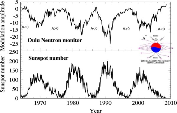
Figure 1. GCR intensity variation as measured by the Oulu neutron monitor (upper panel). The sunspot number is displayed in the lower panel of the figure (SIDC Team 2009, http://sidc.oma.be). From that figure it is evident that the intensities of GCRs and solar activity are anticorrelated. The inset sketches the Sun's magnetic field configuration during an A < 0 solar magnetic epoch.
Download figure:
Standard image High-resolution imageThe time-dependent cosmic ray transport equation derived by Parker (1965) has been solved numerically with increasing sophistication and complexity (Jokipii & Kóta 1995; Burger et al. 2000; Ferreira & Potgieter 2004; Scherer & Ferreira 2005; Alanko-Huotari et al. 2007). The intensity profile as a function of the tilt angle α is displayed in Figure 2 (left) for positively charged particles for three different energies (Potgieter et al. 2001). As expected, the intensity is sensitive to the variation of the tilt angle α in an A < 0 solar magnetic epoch if α is low. In contrast, in an A > 0 solar magnetic epoch it becomes sensitive to α above a threshold of about 60°. These models also predict that the intensity around solar minimum, when the tilt angle is small, for high energies is higher during the A < 0 than during the A > 0 magnetic epochs (see the upper panel of Figure 2 (left)). The opposite is true at higher tilt angles and lower energies. Note that similar tilt dependences are observed when using different ions (α particles) than proton and rigidity instead of the kinetic energy (Webber et al. 2005).

Figure 2. Left: cosmic ray proton intensities at Earth as a function of tilt angle at 2.2 GeV, 430 MeV, and 43 MeV, computed with a steady-state drift model for A > 0 (solid lines) and A < 0 (dashed lines) cycles, respectively (Potgieter et al. 2001). Right: 26-day averaged count rates of 1.2 GV GCR electrons from the MEH experiment onboard ICE (black curve) and helium from the GME (red curve) aboard IMP-8 from 1980 to 1990. The sunspot number (black) and the tilt angle (red) of the solar magnetic field are displayed in the lower panel of the figure.
Download figure:
Standard image High-resolution imageThese predictions from the propagation models including drifts have been proven to be correct when simultaneous measurements of GCR electrons and helium became available in the 1980s for solar cycle 21. The intensity time profiles of 1.2 GV electrons (red curve) and 1.2 GV helium (black curve) for 1980s solar cycle are displayed in the upper panel of Figure 2 (right). The helium and electron measurements are from the MEH (Meyer et al. 1978) and Goddard Medium Energy Experiment (GME; http://spdf.gsfc.nasa.gov/imp8_GME/GME_instrument.html) aboard ICE and IMP-8, respectively. While the electrons recovered to solar minimum values in 1986, the helium intensity increased until 1987 and decreased with solar activity, as shown in the lower panel, where sunspot number and tilt angle α are displayed. Because electrons drift for A < 0 into the inner heliosphere over the poles and out along the HCS, they do not experience variations in α when the latter is below ∼25° (Heber et al. 2002). Since all other propagation parameters are independent of the charge of the particles, the differences in the time profiles of two consecutive solar cycles with opposing polarities can be attributed to charge-dependent drifts. In the 1990s A > 0 solar magnetic epoch, similar measurements have been reported (Heber et al. 2002).
The current solar minimum is remarkable in many ways. Recently, both the Ulysses Team observing the solar wind as well as the radio wave instrument team reported the lowest solar wind densities ever measured (McComas et al. 2008; Issautier et al. 2008). In addition, the magnetic field strength was found to be lower than in the previous solar minimum (Smith & Balogh 2008). Although the sunspot number has been decreasing over the last three years, Figure 1 shows that the GCR intensities do not rise as steep as expected. In order to interpret this "unusual" modulation, we investigate the GCR intensity time profiles of protons and electrons simultaneously during the current solar minimum using Ulysses Cosmic ray and Solar Particle INvestigation/Kiel Electron Telescope (COSPIN/KET) data and compare it with the observations during the 1980s solar cycle.
2. INSTRUMENTATION AND OBSERVATIONS
Ulysses was launched on 1990 October 6, closely before the declining activity phase of solar cycle 22. A swing-by maneuver at Jupiter in 1992 February placed the spacecraft into a trajectory inclined by 80° with respect to the ecliptic plane (Wenzel et al. 1992). Since then the spacecraft is orbiting the Sun with an inclination of about 80 2. The radial distance and heliographic latitude of the spacecraft are shown in the lower panel of Figure 3. From late 1990 to early 1992 the radial distance r to the Sun is increasing from 1 AU to 5.3 AU while the heliographic latitude ϑ is lower than 10°. After the swing by at Jupiter r is again decreasing while ϑ is increasing. Ulysses reached its highest heliographic latitude of 802 south in 1994 September. Within one year the spacecraft scanned the region from highest southern to northern latitudes and was at 802 north in 1995 August. These so-called fast latitude scans have since then repeated from 2000 to 2001 and 2006 to 2007 and are marked by shadings in Figure 3.

Figure 3. From top to bottom are shown the sunspot number, tilt angle α, the solar polar magnetic field strength of the northern and southern polar cap, and the radial distance and heliographic latitude of Ulysses. Marked by shading are the three Ulysses fast latitude scans. The first and third one took place at solar minimum and the second one under solar maximum conditions.
Download figure:
Standard image High-resolution imageThe upper two panels display the sunspot number (black curve) together with the tilt angle α of the HCS (red curve) and the solar polar magnetic field strength over the northern (blue curve) and southern (red curve) polar regions of the Sun. In the 1990s the field strength is positive over the northern and negative over the southern polar regions and vice versa in the 1980s and 2000s. Thus, Ulysses first and third fast latitude scans took place at solar minimum conditions during A > 0 and A < 0 solar magnetic epochs, respectively.
According to the in situ measurements the absolute magnetic polar field strengths were by a factor of 1.5 (north) and 2.2 (south) larger in 1994/1995 compared with 2006/2007. The second fast latitude scan took place during solar maximum when the sunspot number and tilt angle were high and the magnetic field strength over both poles was close to 0.
The observations were made with the KET aboard Ulysses. It measures protons and helium in the energy range from 6 MeV nucleon−1 to above 2 GeV nucleon−1 and electrons in the energy range from 3 MeV to a few GeV (Simpson et al. 1992). The following three particle channels from the KET will be used in this paper.
- 1.Protons from 0.038 to 0.125 GeV (0.194–0.367 GV).
- 2.Electrons from 0.9 to 4.6 GeV (0.9–4.6 GV).
- 3.Protons from 0.25 to 2 GeV (0.549–2.43 GV).
The latter two channels roughly correspond to the same average characteristic rigidity (cf. Rastoin 1995, and values in brackets above) and will be abbreviated as "2.5 GV electrons" and "2.5 GV protons" (see also Heber et al. 1999).
Thus, when comparing Ulysses GCR measurements with those in the 1980s (see Figure 1) we need to take into account that
- 1.KET measurements have to be corrected for a radial gradient and possible latitudinal gradient,
- 2.due to the reduced data coverage in 2008 the statistics in the 1.2 GV electron channel is low. Since the 2.5 GV electron channel corresponds to a broad energy range, we will use this channel.
Figure 4 shows Ulysses daily averaged count rates of 38–125 MeV protons (top panel), and 52 day averaged quiet time variation of the count rates of ∼2.5 GV protons (black curve) together with those of 2.5 GV electrons (red curve) from 1990 November to 2008 December. The latter two are presented as percental changes with respect to the rates Cm, 0.36 counts s−1 for protons and 6.9 × 10⁻⁴ counts s−1 for electrons, measured in mid-1997 at solar minimum, (C(t) − Cm)/Cm. Quiet time profiles have been determined by using only time periods in which the 38–125 MeV proton channel showed no contribution of solar or heliospheric particles (Heber et al. 1999). The observed variations in the 2.5 GV particle intensity are caused by temporal as well as spatial variations due to Ulysses' trajectory. Thus, before discussing the significance of the temporal variation in Figure 4 in detail it is important to understand the role of spatial variations along the Ulysses trajectory. Marked by shadings are again the three different fast latitude scans. These periods will be discussed in more detail in the following section.
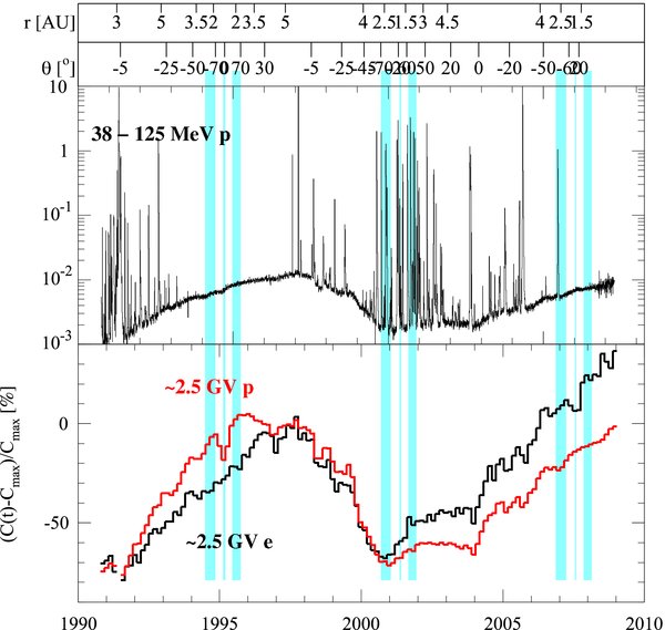
Figure 4. From top to bottom are shown the daily averaged count rates of 38–125 MeV protons from 1990 to 2009 and the 52-day averaged quiet time count rates, given as percental changes, of ∼2.5 GV electrons and protons (red curve). Ulysses radial distance and heliographic latitude are shown on top. Marked by shadings are the three fast latitude scans as defined in Figure 3.
Download figure:
Standard image High-resolution image3. DATA ANALYSIS
The changes caused by solar activity, latitude, and radial distance presented in Figure 4 do not occur in phase, the Ulysses observation will allow us to draw conclusions about the differences in the time profiles of electrons and protons.
Radial gradients. We have shown in previous studies (Heber et al. 1996, 1999, 2002, 2008; Clem et al. 2002; Gieseler et al. 2007) that we can determine mean latitudinal and radial gradients of protons and electrons by either comparing with Earth orbiting experiments or investigating of the electron-to-proton ratio.
- 1.The radial proton gradient varies from about 2.2% AU−1 for the period up to early 1998 to 3.5% AU−1 thereafter (Heber et al. 2002).
- 2.The radial for electrons and protons has been nearly the same from 1992 to 1994 (Clem et al. 2002).
We assume that at a given time the radial gradients of 2.5 GV electrons and protons are approximately the same. Since Chen & Bieber (1993) have shown for GV protons that there is no evidence for a strong variation of the radial gradient with solar magnetic polarity, we will use a mean radial gradient of about Gr = 3% AU−1 for both solar magnetic epochs. Thus, the gradient is somehow over and underestimated during the A > 0 and A < 0 solar magnetic epochs, respectively. Figure 5(left) displays, in the upper and lower panels, the variation of the 2.5 GV proton and electron count rate. The red curves result from correcting Ulysses proton and electron measurements for radial variation with Gr = 3% AU−1.

Figure 5. Upper and lower panels display 52 day averaged quiet time count rates of 2.5 GV protons and electrons, respectively. The left panels show the uncorrected data (black curves) and those corrected by the radial variation of Ulysses with a radial gradient of 3% AU−1 (red curve). The right panels show the latter curves (red, becoming black within the shadings) together with (red curves within the shadings) the count rates being additionally corrected by the latitudinal variation of the spacecraft with latitudinal gradients of 0.3% deg−1 and 0.2% deg−1 for protons and electrons (Heber et al. 1996, 2002, 2008). Marked by blue shading are the two Ulysses solar minimum latitude scans, the yellow shading within these regions indicate time periods in which the count rates show dependences on latitude.
Download figure:
Standard image High-resolution imageLatitudinal gradients. In order to compare the electron with the proton time profiles we have to correct the 2.5 GV proton and electron count rates for latitudinal gradients during the A > 0 and A < 0 solar magnetic epochs, respectively. While the corrected 2.5 GV proton rates show a clear dependence with latitude from 1993 to 1997 (cf. yellow regions in Figure 5 (left)), no correlation during the 2006–2007 solar minimum fast latitude scan was found (Gieseler et al. 2007; Heber et al. 2008). Electrons in contrast show no variation during the 1994/1995 fast latitude scan but a dependence during that in 2006/2007 as again marked by the yellow regions in Figure 5 (left) (Heber et al. 2008). In previous studies, Belov et al. (2001) and Heber et al. (2002, 2003, 2008) found the following.
- 1.The variations of the proton intensity with latitude until mid-1999 are consistent with a vanishing latitudinal gradient in the streamer belt and an average gradient of about 0.25% deg−1 for latitudes above about ±25°.
- 2.In contrast to this behavior the latitudinal gradient decreases markedly to small values after mid-1999, leading to a spherically symmetric intensity distribution around solar maximum conditions and during the A < 0 solar magnetic epoch.
- 3.The variation of the electron intensity with latitude is consistent with a zero latitude gradient until 2003. During the third fast latitude scan Heber et al. (2008) found an average gradient of about 0.19% deg−1.
The time profiles shown in Figure 5 (right) were corrected for a latitudinal gradient Gt = 0.25% deg−1 and Gt = 0.19% deg−1 for protons and electrons, respectively. While the proton gradient has only been applied during the 1990 solar minimum, when the spacecraft was above 25° latitude, the electron gradient was used only during the same conditions in the 2000 solar minimum. Figure 6 shows in the middle panel the radial distance and heliographic latitude of Ulysses. The upper and lower panels display the uncorrected and corrected 2.5 GV electron and proton (red curve) variations, respectively. The calculation of these variations will be explained in the next paragraph. However, the figure also gives a summary of our corrections, showing no obvious intensity variation with Ulysses' latitude or radius in the lower panel. Like the Oulu neutron monitor (see Figure 1), the recent recovery toward solar minimum values occurred in four modulation steps: the increase in the GCR intensities starts after the solar activity period in October to 2003 November (Klassen et al. 2005) and reaches again a plateau in late 2004 before the ground level event in 2005 January (Simnett 2006). Similar step-like time profiles were observed in 2005 and 2007. Therefore, the corrected proton and electron fluxes as derived in this section will be referenced as the "1 AU equivalent" count rate.
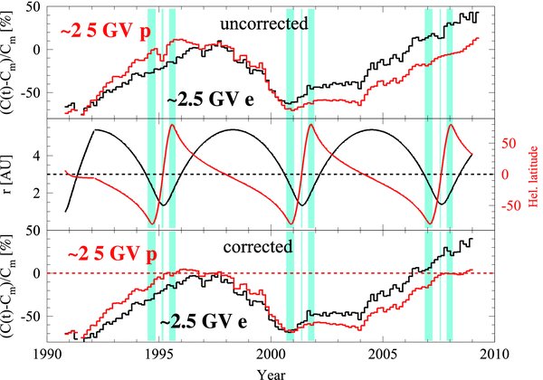
Figure 6. Top and bottom panels display the 52-day averaged quiet time uncorrected (top) and corrected 2.5 GV electrons (black) and proton count rates (red) from Figure 5. The middle panel shows the radial distance (black) and the latitude (red) of Ulysses.
Download figure:
Standard image High-resolution imageTemporal modulation. The third panel of Figure 6 shows the "1 AU equivalent" normalized count rates of 2.5 GV electrons (black curve) and protons (red curve). The "1 AU equivalent" normalized count rate ξ(t) and modulation amplitudes ζ are given by the expressions
where C(t), Cmin, and Cmax are the count rates being time averaged over 52 days at time t, the periods of solar minimum and maximum as defined below, respectively. Thus, the modulation amplitude for the two solar minima and maxima have been determined by

For the time periods we choose C1990 from day of year (DOY) 300 1990 to DOY 35 1991, C1997 from DOY 43 1997 to DOY 243 1997, C2000 from DOY 198 2000 to DOY 348 2000, and C2008 from DOY 26 2008 to DOY 226 2008. Although these periods are chosen somehow arbitrarily, the uncertainty of the values summarized in Table 1 is less than 5% when using fits to the data for slightly different time intervals. During the A > 0 solar magnetic epochs the modulation amplitudes are larger for protons (70% and 67%) than for electrons (64% and 62%). The difference is, however, larger than expected from the calculation, presented in Figure 2 (left). The reason for this discrepancy is the count rate of electrons in 1997. Heber et al. (1999) showed in their Figure 3 that electrons increased for only short periods in 1997 to solar minimum values. When we normalize the electrons to this time period, values of 69% and 67% are found. These values are given in brackets in Table 1. Thus, the electron amplitude and the proton amplitude become the same as predicted by modulation models (Potgieter et al. 2001).
Table 1. Modulation Amplitude for Protons and Electrons with Mean Rigidities of 2.5 GV
| Period | Amplitude Protons (%) | Amplitude Electrons (%) |
|---|---|---|
| ζ(1)+ | 70 | 64 (69) |
| ζ(2)+ | 67 | 62 (67) |
| ζ− | 70 | 92 |
Notes. The number in brackets are the result when using a shorter period in 1997 as reference. For details see the text.
Download table as: ASCIITypeset image
In contrast to the last solar minima in 1987 (see Figure 2 (right)) and 1996/1997 protons and electrons are not recovering to the same values by the end of 2008. Not only does the intensity of 2.5 GV electrons exceed the proton intensity by about 30%, but also the "1 AU equivalent" normalized electron count rate is exceeding the 1997 value by approximately the same amount. In what follows, we show that this observation can be interpreted in the context of the compound model by Ferreira & Potgieter (2004) using a complex dependence of the diffusion tensor and the drift term on the heliospheric field strength and the tilt angle of the HCS.
4. DISCUSSION
By solving Parker's transport equation numerically, Potgieter & Ferreira (2001) and Ferreira & Potgieter (2004) showed that the variation in the GCR intensity can be described by a diffusion coefficient along the heliospheric magnetic field which varies as
with n(α, P) being a number depending on the particle rigidity P (momentum per charge) and the tilt angle α (Potgieter & Ferreira 2001; Ferreira & Potgieter 2004), B(t) and B0 the magnetic field strength at time t and at solar minimum, respectively. n(α, P) = α(t)/α0 where α(t) is the observed time-varying tilt angle and α0 is a "constant" for a given rigidity. The results from Potgieter & Ferreira (2001) and Ferreira & Potgieter (2004) are presented in Figure 7. The Figure demonstrates that a good reproduction of the 22 year cycle for 1.2 GV helium and electrons could be achieved for α0 between 7° and 15°. Note that, as described in Ferreira & Potgieter (2004), the tilt is propagated out into the heliosphere with a solar wind velocity of 400 km s−1 and that using α as a time-dependent factor in the exponent of n, modulation barriers are taken into account. For κ⊥ the same values have been used as in Ferreira & Potgieter (2004). However, at neutron monitor rigidities the authors could demonstrate that in agreement with Wibberenz et al. (2002) n becomes 1. In addition to the model used by Wibberenz et al. (2002), the models by Ferreira & Potgieter (2004), Ferreira & Scherer (2006), and Ferreira et al. (2008a, 2008b) take into account drifts and are therefore better suited to describe the particle transport in the heliosphere around solar minimum conditions.
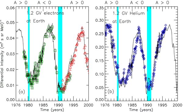
Figure 7. Charge-sign-dependent simulation over two solar cycles using the compound model from Ferreira & Potgieter (2004). Left: computed 1.2 GV electron intensity at Earth compared with observations from ISEE 3/ICE (Clem et al. 2002) and Ulysses (Heber et al. 2003). Right: computed 1.2 GV helium intensity at Earth compared with IMP-8 measurements (McDonald et al. 1998).
Download figure:
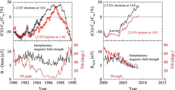
Standard image High-resolution imageIn Figure 8, we compare the normalized count rates of 1.2 GV electrons and helium for the 1980s A < 0 solar magnetic epoch (left) with the "1 AU equivalent" normalized 2.5 GV electron and proton count rate (right) during the 2000s A < 0 solar magnetic epoch. 1.2 GV particles have been normalized by using values (0.2 counts s−1 for helium and 20 counts s−1 for electrons) so that the solar maximum value in 1991 reached −70% (not shown here). Using this normalization, the count rates of both helium and electrons reach a value of 35%–40% in 1986. During the same time the heliospheric field strength decreased from about 8 nT around solar maximum to 5 nT at solar minimum. While the tilt angle α was below 10° from 1985 to 1987, the electron count rate was more or less constant and the helium count rate increased from 0% to 30% from 1986 to 1987, only. Solar activity increased again in early 1987 with first the tilt angle increasing to values of 25°–30° in 1988. In agreement with the model calculation by Ferreira & Potgieter (2004) the normalized count rate of helium decreased again to 0%. Later, both the heliospheric magnetic field strength and the tilt angle increased and also both electrons and helium were decreasing until 1990 when solar maximum was reached.
Figure 8. Left: long-term averaged normalized count rates of 1.2 GV GCR electrons (black curve) and helium (red curve) from 1980 to 1990. The count rates have been normalized so that a value of −70% are determined in 1991 (not shown here). Right: 56 day averaged normalized count rates of 2.5 GV electrons and protons from 2000 to 2009. The heliospheric magnetic field strength from the Omni tape and the ACE spacecraft (Stone et al. 1998) as well as the tilt angle (red curve) are displayed in the lower panels. As discussed in detail by Heber et al. (2002) the tilt angle has been shifted by 78 days in order to account for the time to establish the propagation conditions in the inner heliosphere.
Download figure:
Standard image High-resolution image
The right part of Figure 8 shows the same parameters, but 20 years later. As mentioned above, 1.2 GV electrons and helium have been substituted by the "1 AU equivalent" normalized 2.5 GV electron and proton count rate channels due to the low statistics in the 1.2 GV electron channel in 2008. Note that at these slightly higher rigidities the modulation amplitude is expected to become smaller. Thus, the absolute values should not be compared between the two solar cycles. The lower panel displays the long-term averages of the heliospheric magnetic field strength and the tilt angle α. As 20 years ago the heliospheric magnetic field strength B was at about 8 nT around solar maximum. From 2005 onward B decreased to values of about 4 nT, i.e., about 1 nT lower than in 1986. The tilt angle α, however, decreased from about 60° to 30° and reached up to now never a value below 20°. During the same period both proton and electron fluxes increased from −50% and −30% to 0% and 30%, respectively.
Comparing the left part with the right part of Figure 8, it is interesting to note that at the end of 1985 and the beginning of 1986 similar differences have been observed. At that time the tilt angle α was still above 20° and the magnetic field strength around 6–7 nT. The normalized helium and electron count rates reached values of about −35% and 0%, respectively. Due to the decrease in B the normalized count rates of both electrons and helium increased. Since the tilt angle quickly decreased from 25° to values below 10°, the increase was much larger for helium than for electrons, reaching the same values in 1987. Thus, we expect the protons to increase to the electron level as far as the tilt angle will become lower than 10°. If the heliospheric magnetic field strength will stay around 4 nT we predict that the GCR proton count rate will increase until they reach the same modulation amplitude than the electrons, resulting in a factor of about 1.3. Since no continuous electron measurements at neutron monitor rigidities have been performed, the intensity variation of the Oulu neutron monitor is more difficult to interpret. By the end of 2008 the intensities of the neutron monitor were higher than those during the 1987- and the 1997 solar minima, although the intensities at 2.5 GV reached only the same values than in the latter. However, if we assume that the diffusion coefficient is the same during both solar magnetic epochs, then it is obvious from Figure 3 (left) that with increasing rigidity the tilt angle when the intensities during A > 0 equals the intensities during the A < 0 solar magnetic epoch moves to higher values. Because the break-even intensity is at about 12° for 1 GV and 25° for 3 GV the intensity for low and high rigidities will be lower and higher when the tilt is between these break-even values. The intensities are in addition depending on the magnetic field strength as discussed above. Thus, the intensities are expected to be larger during the current solar minimum, compared with the other solar minima, as observed by the Oulu neutron monitor. Since no measurements of 2.5 GV are available to us for the 1987 solar minimum, the absolute variation between these cycles should not be compared. Thus, we would expect to observe the highest GCR intensities ever measured in heliospheric space.
5. SUMMARY AND CONCLUSION
Based on COSPIN/KET measurements obtained with Ulysses from launch in 1990 October to the end of 2008, we present in this paper electron and proton count rates for a rigidity of ≈2.5 GV. The data set covers the recovery phases of solar cycles 22 and 23 as well as other phases of solar cycle 23. We obtain the "1 AU equivalent" count rates by disentangling variations related to solar activity and the varying radial distance and latitude along the Ulysses orbit, using radial and latitudinal gradients determined by Heber et al. (1996, 1999, 2002), Clem et al. (2002), Gieseler et al. (2007), and recently Heber et al. (2008). In detail
- 1.The radial gradient can be approximated for electrons and protons by about 3% AU−1.
- 2.The variation of proton intensity with latitude is consistent with a vanishing latitude gradient in the streamer belt and an average gradient of about 0.25% deg−1 for latitudes above about ±25° until mid-1999. The latitudinal gradient decreases markedly to small values after mid-1999, leading to a spherically symmetric intensity distribution since then.
- 3.Based on the observed latitudinal proton intensity variations, the corresponding gradient of electrons could be determined from 2005 to 2008. A gradient of 0.19% deg−1 has been applied.
The comparison of the corrected proton count rates with neutron monitor observations resulted in the same modulation features. Thus, the corrected measurements can be used as "1 AU equivalent" electron and proton count rates. Although the sunspot number and the heliospheric magnetic field strength reached solar minimum values in 2008 the count rate of electrons exceeded the proton count rate by about 30%. During the 1980s, when first long-term charge-sign-dependent measurements became available, both electron and proton count rates reached the same level at solar minimum early 1987. In contrast to the period in 2008, the tilt angle, i.e., the maximum latitudinal extent of the HCS, was in 1986 below 10°. This leads us to the conclusion that curvature and gradients drifts, as predicted by Ferreira & Potgieter (2004), prevent the proton count rates to reach real solar minima level, because the particles have to drift into the heliosphere along the HCS, while the electrons already reached their solar minimum intensities. Therefore, the proton intensity is still lower than expected. Another important conclusion for the current solar cycle 23 minimum is that the proton intensity will increase by ∼30% and will reach the highest intensities ever measured in heliospheric space, if the tilt angle will decrease below 10°. This work also shows the importance of simultaneous measurements of protons and electrons in order to understand the modulation of GCRs in the heliosphere. On the other hand, the work by Ferreira & Potgieter (2004) implies that such measurements could be interpreted correctly only if our model takes into account all physical transport processes in the heliosphere.
The Ulysses/KET project is supported under grant 50 OC 0105 and 50 OC 0902 by the German Bundesministerium für Wirtschaft through the Deutsches Zentrum für Luft- und Raumfahrt (DLR). M.S.P. and S.E.S.F. acknowledge the partial financial support of the SA National Research Foundation and the SA Centre for High Performance Computing. The German–South African Collaboration has been supported by the DLR under grant SUA 07/013. This work profited from the discussions with the participants of the ISSI Team meeting "Transport of Energetic Particles in the Inner Heliosphere." Wilcox Solar Observatory data used in this study was obtained via the Web site http://wso.stanford.edu, courtesy of J. T. Hoeksema.