


ABSTRACT
We present a morphology study of intermediate-redshift (0.2 < z<1.2) luminous infrared galaxies (LIRGs) and general field galaxies in the GOODS fields using a revised asymmetry measurement method optimized for deep fields. By taking careful account of the importance of the underlying sky-background structures, our new method does not suffer from systematic bias and offers small uncertainties. By redshifting local LIRGs and low-redshift GOODS galaxies to different higher redshifts, we have found that the redshift dependence of the galaxy asymmetry due to surface-brightness dimming is a function of the asymmetry itself, with larger corrections for more asymmetric objects. By applying redshift-, infrared (IR)-luminosity- and optical-brightness-dependent asymmetry corrections, we have found that intermediate-redshift LIRGs generally show highly asymmetric morphologies, with implied merger fractions ∼50% up to z = 1.2, although they are slightly more symmetric than local LIRGs. For general field galaxies, we find an almost constant relatively high merger fraction (20%–30%). The B-band luminosity functions (LFs) of galaxy mergers are derived at different redshifts up to z = 1.2 and confirm the weak evolution of the merger fraction after breaking the luminosity–density degeneracy. The IR LFs of galaxy mergers are also derived, indicating a larger merger fraction at higher IR luminosity. The integral of the merger IR LFs indicates a dramatic evolution of the merger-induced IR energy density [(1 + z)∼(5−6)], and that galaxy mergers start to dominate the cosmic IR energy density at z ≳ 1.
Export citation and abstract BibTeX RIS
1. INTRODUCTION
Our understanding of galaxy formation and evolution has advanced dramatically in the past decade, with well-determined cosmic evolution of the comoving star formation density, galaxy stellar mass, and galaxy metallicity content (see Cowie & Barger 2008, and references therein). What mechanism drives this evolution? Galaxy interactions and mergers play a key role in the theory of galaxy evolution, through transforming the galaxy morphologies, inducing violent starbursts, and feeding the central massive black holes (Mihos & Hernquist 1996; Springel et al. 2005). However, it is still unclear from observations to what extent galaxy mergers actually play the roles predicted for them.
Galaxy mergers can be found from observations either morphologically or kinematically. Morphologically identified mergers include galaxies with tidal tails, wisps, and/or multiple nuclei. They can be found through either visual classifications or quantitative measurements. While visual classification is the testbed to develop the quantitative methods, it is time consuming to classify the enormous numbers of galaxies found in deep surveys. Moreover, distant galaxies can change their apparent morphologies due to surface-brightness (SB) dimming. Such an effect can be corrected better through quantitative measurements. Several quantitative morphology techniques have been developed, CAS (Abraham et al. 1994, 1996; Conselice et al. 2000, 2003) and Gini-M20 (Abraham et al. 2003; Lotz et al. 2004). They classify mergers by identifying galaxies in a predefined parameter space. Although the interpretation of the parameter space is somewhat uncertain, studies based on the same quantitative definition can be compared and are less subjective than visual classification. Galaxy mergers can also be identified through kinematical pairs of galaxies or galaxies with complicated internal velocity fields (i.e., neither pressure nor rotationally supported). Identifying them requires time-consuming spectroscopic observations, which have been conducted for only a limited number of objects (de Ravel et al. 2008; Neichel et al. 2008).
Different approaches to merger identification are sensitive to different stages of the galaxy merging process. Pair-identification algorithms find separated interacting galaxy pairs while the morphologically based algorithms usually identify galaxies during the first pass and final coalescence where the galaxy morphology is significantly disturbed by gravitational torques (Lotz et al. 2008b). Galaxy mergers with complicated interval velocity fields seem to span a longer timescale of the merging process (Neichel et al. 2008). Nevertheless, no method can identify all mergers. In addition, a fraction of galaxies identified as mergers by any method are not necessarily major mergers. For example, minor mergers of gas-rich galaxies can also have highly disturbed morphologies (J. M. Lotz et al. 2009, in preparation).
Morphology studies of high-redshift galaxies show that the Hubble sequence is in place by z ∼ 1 and that high-redshift galaxies are associated more frequently with peculiar features (e.g., Brinchmann et al. 1998). Some studies have found that the galaxy merger fraction shows strong redshift evolution, characterized by (1 + z)m with m > 2 (e.g., Le Fèvre et al. 2000; Patton et al. 2002; Conselice et al. 2003; Cassata et al. 2005; de Ravel et al. 2008), implying that the cosmic star formation history (SFH) is at least partly driven by galaxy mergers. Other studies, however, found a slow evolution (e.g., Bundy et al. 2004; Lin et al. 2008; de Ravel et al. 2008) or even no evolution (Lotz et al. 2008a). The discrepancies among different studies may be caused by low-number statistics, morphological K-corrections (e.g., Papovich et al. 2003), the method to identify mergers (Lotz et al. 2008b) and the physical properties (e.g., gas fractions) of merger progenitors (Lotz et al. 2008b). Nevertheless, almost all studies have found relatively low merger fractions (less than 20%) at z< 1.
A more direct way to constrain the role of galaxy mergers in the cosmic SFH is to investigate morphologies of luminous infrared galaxies (LIRGs; LIR > 1011 L☉). LIRGs show strong redshift evolution and start to dominate the cosmic infrared (IR) energy density at z > 0.7 (Le Floc'h et al. 2005; Pérez-González et al. 2005). In the local universe, LIRGs are mainly (∼50%) triggered by major mergers (Sanders & Mirabel 1996). However, morphology studies of intermediate-redshift LIRGs indicate low merger fractions (∼10%–30% Zheng et al. 2004; Bell et al. 2005; Bridge et al. 2007; Lotz et al. 2008a; Melbourne et al. 2008). These findings have led to claims that the cosmic SFH is driven by some less violent mechanisms, such as accretion or gas consumption (Noeske et al. 2007; Daddi et al. 2008).
In Shi et al. (2006), we measured the galaxy asymmetry for LIRGs in the Ultra Deep Field (UDF), which provides limiting SB for galaxies at z= 1 comparable to that often obtained for local ones (μB = ∼25.3 mag arcsec−2 at 10σ in the AB magnitude system). The merger fraction obtained in this study is several times higher than others, 40% ± 24% and 26% ± 10 % for LIRGs and general field galaxies (MB < −19.25) at z∼0.7, respectively. The comparison (see Figure 1) between asymmetry measurements using the GOODS images and ones using the UDF images for the same galaxies indicates substantial deficits in the indicated asymmetry in the shallower GOODS images. These two results motivate us to suspect that other studies based on relatively shallow imaging (most of which are shallower than GOODS) may underestimate significantly the role of SB dimming in galaxy morphology measurements. If so, the role of mergers in triggering luminous episodes of star formation may be seriously underestimated.

Figure 1. Comparison of galaxy morphologies using the GOODS z-band images and the UDF z-band images for about 250 UDF objects with relatively high S/N and large size. The median error bar is shown in bottom-right corner. The solid line is for Asy(GOODS) = Asy(UDF).
Download figure:
Standard image High-resolution imageTo test the result of Shi et al. (2006) with much higher statistical significance and better constrain the role of galaxy mergers in the cosmic SFH, in this paper we carry out detailed asymmetry measurements and corrections for all galaxies (∼16,000) with mz< 25 including ∼7500 galaxies and ∼1000 LIRGs at z< 1.2 in the GOODS field. In Section 2, we describe our revised asymmetry estimate method. In Section 3, data for a complete local LIRG sample and the GOODS ACS, redshift, and Spitzer observations are presented, as well as the concentration and asymmetry measurements for both local LIRGs and GOODS galaxies. Section 4 shows the evolution of the observed asymmetries of GOODS galaxies (Section 4.1) and the results after asymmetry corrections, including the redshift evolution of the merger fraction in LIRGs (Section 4.2), the evolution of the merger fraction in general field galaxies (Section 4.3), and the IR and rest-frame B-band luminosity functions (LFs) of galaxy mergers (Section 4.4). In Section 5, we discuss the role of mergers in galaxy star formation activity since z ∼ 1. The conclusions are in Section 6. The technical details are given in Appendix A for our revised asymmetry method and in Appendix B for asymmetry deficits of redshifted local LIRGs and low-z (z = 0.2–0.4) GOODS galaxies due to SB dimming. Throughout the paper, we adopt a cosmology with H0= 70 km s−1 Mpc−1, Ωm= 0.3, and ΩΛ= 0.7. All magnitudes are defined in the AB magnitude system.
2. GALAXY STRUCTURE MEASUREMENT
2.1. Galaxy Size and Concentration
Quantitative galaxy morphologies are always measured within well-defined apertures in order to probe the same physical regions of galaxies; these apertures are optimized to include as much galaxy flux as possible while minimizing the effect of noise plus SB dimming. When comparing low- to high-redshift galaxy morphologies, SB dimming (SB ∝(1 + z)4) can artificially decrease the galaxy size. To avoid such an effect, the galaxy size can be measured through the dimensionless parameter:

where I(r) is the SB at radius r and 〈I(r)〉 is the mean SB within radius r (Petrosian 1976). In the standard approach (Conselice et al. 2000, 2003), the Petrosian radius Rp is defined at η(r)= 0.2 and the galaxy aperture radius is defined to be 1.5 Rp. The SB I(r) can be measured within either circular apertures or elliptical apertures. For inclined noninteracting galaxies, the mean galaxy ellipticity and position angle trace the true galaxy light well. The Rp defined within an elliptical aperture is generally larger than that defined within a circular aperture and can be two times larger for extremely inclined systems. However, we have found that interacting galaxies usually have large variations in their position angles and ellipticities. The measured galaxy size for them depends on the adopted position angle and ellipticity. Because of this uncertainty for the interacting systems, we adopt circular apertures universally for all galaxies in this paper. For most local LIRG systems, we found that the difference in Rp between circular apertures and elliptical apertures with mean ellipticity and position angle is within 20%. Therefore, using circular apertures does not introduce large errors.
The concentration parameter measures how compact the light distribution is. It has been shown to correlate well with the Hubble type (Kent 1985; Bershady et al. 2000). Early-type galaxies generally have more compact light distributions than do late-type ones. With the curve of growth measured within the galaxy aperture, the concentration can be defined as the ratio of the two radii enclosing two fixed fractions of the light. Following Kent (1985) and Bershady et al. (2000), we have used the following definition in this paper:
where R80 and R20 are the radii that enclose 80% and 20% of the total light, respectively.
2.2. Revised Asymmetry Parameter
The asymmetry parameter (A) was first introduced by Abraham et al. (1996) and subsequently developed by Conselice et al. (2000, 2003). It quantitatively describes the level of the galaxy asymmetry and provides a direct measurement of the importance of asymmetric substructures in galaxy morphologies, such as merging companions and tidal tails, which are used to identify mergers in visual classification. Accurate measurements of the asymmetry parameter are thus critical to understand the role of galaxy mergers in galaxy evolution. The galaxy asymmetry is defined as
where Agalaxy+noise is the asymmetry of the galaxy signal plus the noise, Igalaxy+noise is the image of galaxy signal plus the noise, and  is Igalaxy+noise with the image rotated by 180° around a rotation center. The true pure galaxy asymmetry is then given by

where min(Agalaxy+noise) is the minimum of the galaxy signal plus noise asymmetry, and Acorrnoise is the noise correction obtained by rotating a background image around a center and normalizing by the galaxy brightness:
where B is the background image without any object.
The overall measurements of galaxy concentration and asymmetry are composed of the following steps:
- 1.Guess the initial center.
- 2.Measure the Rp and concentration.
- 3.Search for the rotation center that gives the minimum of Agalaxy+noise within a 1.5 Rp aperture.
- 4.Use the new rotation center to remeasure the Rp and concentration.
- 5.Use the above rotation center and new Rp to search for a new rotation center that gives the minimum of Agalaxy+noise within a 1.5 Rp aperture.
- 6.Correct for the noise Acorrnoise.
The galaxy centers can be easily located for noninteracting galaxies but not for interacting ones. Here, we adopt the rotation center giving the minimum of Agalaxy+noise to measure the galaxy size as is done in steps 1–3. Note that the asymmetry rotation center in step 5 is usually not very different from that in step 3, as the "walking around" method invented by Conselice et al. (2000) is generally robust to find the minimum Agalaxy+noise. For discussions about the galaxy size definition, the algorithm searching for the minimum Agalaxy+noise, and the dependence of Agalaxy+noise on the resolution and correlated noise, see Conselice et al. (2000, 2003).
The technical details about our new Acorrnoise are given in Appendix A. Here, we present a summary of the procedure to determine this parameter. A set of 1000 randomly produced noise asymmetry measurements is carried out by putting circular regions in the background image around the target. The value of this distribution at the 15% probability low-end tail is used as Acorrnoise, the median of true noise corrections. The error (∼3σ) in the final measured galaxy asymmetry is taken to be two times the standard deviation of these randomly produced noise asymmetries. In reality, some galaxies are always present in the field of targets. To account for this problem, a success rate is defined for the 1000 circular region placements as the fraction of circular regions containing no galaxy signal indicated by the SExtractor segmentation image. Circular regions containing any galaxy signal are not used. More sets of 1000 placements are generated until 1000 successful measurements are reached. If the success rate for one set of 1000 placements is lower than 50%, the circular region size for the following set is taken to be 80% of this set. Then, the measured noise asymmetry is rescaled to that with the original size by assuming that the noise asymmetry is proportional to the aperture area.
3. GALAXY SAMPLE
3.1. Local LIRG Sample
Local LIRGs and ultra-luminous infrared galaxies (ULIRGs) are generally galaxies undergoing mergers with morphological signatures of tidal tails, multiple nuclei, and highly asymmetric features (Sanders & Mirabel 1996). To account for the redshift dependence of galaxy merger morphologies due to SB dimming, we measured the morphologies of local LIRGs and of local LIRGs redshifted to different redshifts. We retrieved Hubble Space Telescope (HST) Advanced Camera for Surveys (ACS)/WFC-F435W images of 88 local LIRGs observed in Program ID-10592 (PI: Aaron Evans). This local LIRG sample is a complete subsample of the IRAS Revised Bright Galaxy Sample (RBGS; i.e., f60 μm > 5.24 Jy; Sanders et al. 2003) above LIR = 1011.4 L☉. The sample size is large enough for statistically valid comparisons. The distance of this sample covers the range from 35 to ∼350 Mpc. The median distance of 135 Mpc corresponds to a physical resolution of 80 pc. These galaxies are also bright enough to be useful when redshifted to higher redshifts. These local LIRGs are currently experiencing merging processes, spanning a wide range of merging stages from well-separated galaxy pairs to the final merging remnants.
To obtain quantitative morphology measurements, foreground stars and background galaxies should be removed from the images first. Given the importance of the background region in accurate morphology measurements (see Appendix A), we carried out a careful removal of contaminators, especially given that some of the LIRGs have tens of foreground stars. We used SExtractor (Bertin & Arnouts 1996) to obtain the segmentation map of each image. To make sure the extended low-SB emission was included in the object, we first rebinned the image by a factor of 4 × 4 and then adjusted the parameters in SExtractor so the extended emission was detected. This segmentation map was then resampled to the original resolution by assuming that the original pixels belonging to a rebinned pixel conserve the segmentation value. We then cleaned the neighborhood of the target by replacing pixels of nontarget object pixels randomly with values of background pixels. As the neighborhood is dominated by the background pixels (greater than 95%), such replacement does not introduce any significant correlation in the final cleaned neighborhood background. Sometimes a target was identified as several different objects by SExtractor. We visually inspected each image to make sure such substructures were still included in the target during the neighborhood clean. Sometimes foreground stars lie within the target region and cannot be separated by SExtractor. We used the IRAF package IMEDIT to remove these contaminators further.
As the local LIRG sample is a flux-limited sample instead of a volume-limited sample, we have applied weights of  /
/ to each object to obtain an equivalent volume-limited asymmetry distribution, where Vmax is measured at the redshift where the object with a given IR luminosity has f60 μm = 5.24 Jy.
3.2. Galaxies in the GOODS Field
3.2.1. HST Images and Morphology Measurements
The GOODS field consists of two subfields, GOODS-North (GOODS-N) and GOODS-South (GOODS-S), imaged with HST/ACS in four filters B (F435W), V (F606W), i (F775W), and z (F850LP) (Giavalisco et al. 2004, M. Giavalisco & the GOODS Team, 2008, in preparation). The field centers (J2000.0) are 12h36m55s, 62°14'15'' for the GOODS-N and 3h32m30s, −27°48'20'' for the GOODS-S. The survey area is 320 arcmin2 with BViz-band coverage and 365 arcmin2 with Viz-band coverage for each field. GOODS version 2.0 provides exposure times of 7200, 5650, 8530, and 24760 s in GOODS-N and 7200, 5450, 7028, and 18232 s in GOODS-S. The final image has a pixel scale of 0 03 pixel−1. The GOODS-S and GOODS-N fields are divided into 18 and 17 sections, respectively. An individual image file is released for each section.
Objects were detected in the z band with the SExtractor package (Bertin & Arnouts 1996) and photometry was measured in all four bands. We produced the segmentation images that define the galaxy pixels using the released parameter files of SExtractor plus weight map images, and final science images. We used galaxy magnitudes defined by SExtractor MAG_AUTO.
We carried out morphology measurements in the Viz bands for 16,708 objects with mz< 25, SExtractor CLASS_STAR < 0.9, FLUX_RADIUS1 < 100, IMAFLAGS_ISO < 16 and not within 33 pixels of the edge of each SECTION field. SExtractor FLUX_RADIUS1 is the radius in pixels enclosing 20% of the flux and FLUX_RADIUS1 < 100 excludes nine artificial objects that are long narrow bright belts across the field. IMAFLAGS_ISO < 16 excludes objects within 33 pixels of the field edge. The morphology measurement was first carried out in z band starting with cutting out science and segmentation images for each object. As the galaxy radius is defined to be 1.5 Rp and the asymmetry uncertainties are measured by putting circular regions randomly in background regions around the objects, the image size was cut out with a size of 9Rp × 9Rp. Then, the z-band concentration and asymmetry were measured as described in Section 2.2. Briefly, the residual sky was first subtracted using the mean values of all pixels with zero segmentation values. Companions were defined as all pixels with nonzero segmentation values not equal to the target's value. They were removed by replacing their pixel values randomly with those of sky pixels. Note that the removed companions are those well separated from targets and thus do not contribute to the target asymmetries. The initial center was given by the astrometrical position of the object. The first set of concentration/asymmetry measurements gave new centers and the second measurements were carried out to give Rp, concentration, and asymmetry values. The asymmetry uncertainty was measured in 1000 circles randomly put in the sky region, excluding object and companions (for details, see the last paragraph of Appendix A). To evaluate the dependence of the asymmetry uncertainties on the signal-to-noise ratio (S/N), two types of S/N are defined. The total S/N is the total signal divided by the total sky noise for galaxy pixels within the 1.5 Rp radii. Note that sky and companion pixels are excluded. Similar to Lotz et al. (2008a), 〈S/N〉 is defined to be the arithmetic (not quadratic) average of the S/N of each galaxy pixel. The asymmetry/concentration measurements failed for 212 objects (175 of them are stars; the remaining 37 objects either have extremely low SB or are near the edge, within 50 pixels). No systematic correction is made for these objects, as the SB limiting cut will be applied in the final morphology catalog and they are a very small fraction (0.2%) of the total number of objects. The Vi-band concentration and asymmetry were then measured for all objects with successful z-band concentration and asymmetry measurements.
3.2.2. Spitzer MIPS and IRAC Data
MIPS and IRAC data for the GOODS-N and GOODS-S fields were drawn from the Spitzer GTO observations of the larger area covering each field, 1 5×05 for MIPS and 10×05 for IRAC. The reduction of the 24 μm images was carried out with the MIPS Data Analysis Tool (Gordon et al. 2005). The detailed data reduction, object detection, and photometry measurement procedures are given in Papovich et al. (2004) and Pérez-González et al. (2005). The final MIPS 24 μm catalog is 50% complete at 60 μJy.
3.2.3. Redshifts and Morphology-Redshift Catalog
For the GOODS-S field, the spectroscopic redshifts were obtained from version 3.0 of the FORS2 catalog (Vanzella et al. 2008) and version 1.0 of the VIMOS catalog (Popesso et al. 2009). Only solid redshifts with redshift quality zq = A were used. For GOODS-N, we used spectroscopic redshifts with zq= 3 or 4 from the Team Keck Treasury Redshift Survey (TKRS) catalog. For objects without secure spectroscopic redshifts, we used the catalog of Pérez-González et al. (2008), who obtained photo-z based on photometry covering from UV to IRAC bands.
The photo-z error σz/(1+z) is <0.2 for 95% of the redshifts and <0.1 for 88% of the redshifts. The median σz/(1+z) is 0.03. The photo-z error is small enough for our purpose, i.e., to determine the rest-frame band of the galaxy image. These redshift catalogs were matched to the GOODS z-band morphology catalog using a search radius of 05. The redshift was assigned to the nearest one if multiple objects were present within a search radius. The redshift completeness for mz< 25 is 68%; it is mostly determined by the IRAC detections for which the photo-z can be calculated in Pérez-González et al. (2008). We refer to the sample of objects with both morphology and redshift measurements as the morphology-redshift catalog.
To account for the morphological K-correction, the redshift evolution of the galaxy morphology was determined in the rest-frame B band for objects at z< 1.2. The redshift range of z< 1.2 was divided into five redshift bins, [0.2, 0.4], [0.4, 0.6], [0.6, 0.8], [0.8, 1.0], and [1.0, 1.2]. The rest-frame B-band morphologies in a given redshift bin were defined as the morphologies in the band nearest to the redshifted rest-frame B band, i.e., the observed-frame V, V, i, i, and z band for the redshift bins from low to high.
To obtain the optical counterparts of the MIPS sources, we first obtained the IRAC 8 μm counterparts using a search radius of 1''. Then for MIPS sources with IRAC counterparts, the optical counterparts were defined as objects in the morphology catalog within 1'' of the IRAC counterparts. For MIPS sources without IRAC counterparts, optical counterparts were searched for within 25 of the MIPS source. For multiple objects within a search radius, the nearest one was defined to be the optical counterpart. For MIPS sources with known optical redshifts, the total 8–1000 μm IR luminosity was obtained based on the observed 24 μm flux density and the star-forming templates from Rieke et al. (2009).
3.3. Reliable Morphology and Completeness Cut
The redshift-morphology catalog was further limited to objects with reliable asymmetry measurements, defined as those with Rgal= 1.5Rp > 15 pixels (003 pixel−1) and error(A) < 0.1 in a given band. The accuracy of the galaxy asymmetry depends on the resolution and S/N. For a galaxy with small size, the resolution is not high enough to resolve galaxy structures and the asymmetry becomes artificially small (Conselice et al. 2000). For galaxies with low S/Ns, the asymmetry uncertainty is large due to the noise. For the study in this paper, we used an asymmetry uncertainty cut (error(A) < 0.1 at approximately 3σ level) instead of an S/N cut, as our revised asymmetry method can characterize the uncertainty due to complicated background structures. Figure 2 shows the advantage of the asymmetry uncertainty cut over the S/N cut. While both S/N and 〈S/N〉 are tightly correlated with the asymmetry uncertainty at high S/N (e.g., 〈S/N〉> 3), the scatter of the correlation becomes large at 〈S/N〉< 3. A high-S/N cut (e.g., 〈S/N〉> 3) will exclude many objects with relatively small asymmetry uncertainty (error(A) < 0.1) and a low-S/N cut (e.g., 〈S/N〉> 1) will introduce objects with large asymmetry uncertainty (error(A) > 0.1). Our error(A) < 0.1 criterion only excludes objects with large asymmetry uncertainties. Most objects with error(A) > 0.1 have relatively inhomogeneous backgrounds. All objects with error(A) > 0.3 are at the edge of the field where the exposure is relatively shallow and shows a large gradient toward the edge.

Figure 2. S/N vs. asymmetry uncertainty (3σ), where the upper panel shows the mean S/N and the lower panel is for the total S/N. The S/N is only correlated with the asymmetry uncertainty for galaxies with 〈S/N〉> 30 and S/N > 3.
Download figure:
Standard image High-resolution imageWe now have a redshift-morphology catalog with redshift information and reliable morphology measurements. The redshift evolution of galaxy morphologies will be characterized in a subsample of this catalog that is complete to a certain value. Figure 3 shows the completeness cut at 50%, 70%, and 90% of the redshift-morphology catalog in Rgal versus magnitude in three bands, where the completeness is defined as the ratio of the number of galaxies with redshift measurements and secure morphologies to the total number of galaxies in an Rgal-magnitude bin. The absolute values at different redshift bins are given in Table 1. Here, we do not account for incompleteness of the HST/ACS catalog, as its incompleteness at mz< 25 is negligible.

Figure 3. Galaxy radius vs. magnitude in v, i, z bands for galaxies selected with mz< 25. Areas with different grayscales correspond to different completeness cuts of galaxies with reliable morphology and redshift measurements (see Section 3.3). The solid lines enclose the 70% complete area where the apparent surface brightness, size, and magnitude are labeled.
Download figure:
Standard image High-resolution imageTable 1. The 70% Completeness Cut of the Morphology-Redshift Catalog Shown in Figure 3
| Redshift | Rgal (kpc) | Mrest B | μrest B (mag kpc−2) |
|---|---|---|---|
| 0.3 | 2.4 | −16.4 | −10.3 |
| 0.5 | 3.3 | −17.5 | −10.7 |
| 0.7 | 3.9 | −18.6 | −11.9 |
| 0.9 | 4.2 | −19.1 | −12.2 |
| 1.1 | 4.4 | −19.8 | −12.4 |
Notes. The apparent galaxy size, magnitude, and surface brightness are labeled in Figure 3. The absolute magnitude is measured as M = m − 5.0log(DL) + 5 + 2.5log(1 + z), where DL is the luminosity distance in pc and 2.5 log(1 + z) is the K-correction (see Section 3.2.3).
Download table as: ASCIITypeset image
Figure 4 shows the absolute magnitude, galaxy size, SB and IR luminosity as a function of redshift for all mz< 25 and MIPS-detected objects with redshift measurements. The absolute rest-frame B-band magnitude is measured through the version 4.1.4 KCORRECT code (Blanton et al. 2003; Blanton & Roweis 2007) using four ACS bands. For the first three quantities, the 70% complete redshift-morphology cut is drawn in each redshift bin and the 50% complete IR flux limit is drawn for the IR luminosity. As shown in the figure, most objects with mz < 25 and z< 1.2 are included in the final redshift-morphology catalog. This is because the incompleteness of the redshift-morphology catalog is mainly caused by the redshift incompleteness instead of the criterion of secure morphologies.
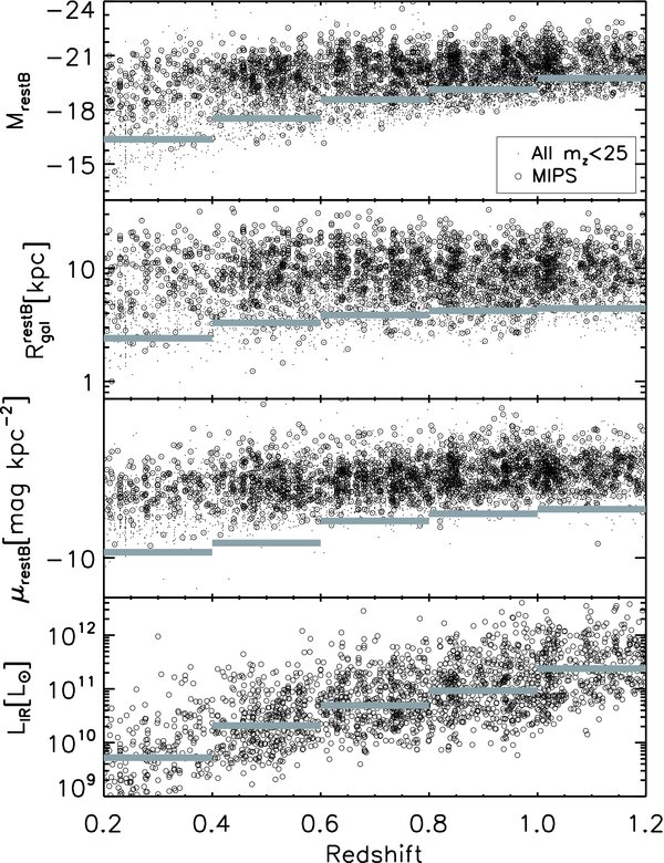
Figure 4. First three panels show the rest-frame B-band magnitude, the galaxy radius, and the rest-frame B-band surface brightness as functions of redshift for all galaxies with mz< 25 (dots) and MIPS-detected galaxies (open circles). The heavy solid lines correspond to the 70% completeness cut of the redshift-morphology sample (see Section 3.3). The last panel shows the total IR luminosity of MIPS-detected galaxies as a function of redshift where the solid lines correspond to the 50% completeness cut of the 24 μm detections.
Download figure:
Standard image High-resolution image4. RESULT
4.1. Observed Asymmetry Distributions of GOODS Galaxies
Two main results described in the Appendices are important for the study of morphology evolution. First, as shown in Appendix A, we found that the underlying structure of the sky background is important in accurate asymmetry measurements and we propose a revised asymmetry measurement approach. Second, by redshifting local LIRGs and low-z (z = 0.2–0.4) GOODS galaxies to higher redshifts, asymmetry deficits due to SB dimming for these two galaxy populations are derived as a function of redshift. As shown in Appendix B, originally more asymmetric objects show larger asymmetry deficits. Such dependence indicates that to recover the intrinsic distribution of a galaxy population at a given redshift, a low-z galaxy population with intrinsically similar asymmetry should be used to construct the asymmetry corrections. Such a low-z galaxy population can be defined through comparing the observed asymmetries of redshifted low-z galaxies to those of the galaxy population at a given redshift, as the observed asymmetries still on average correlate with original asymmetries even given the larger asymmetry deficits for originally more asymmetric objects (see Figure 1).
Figure 5 shows the observed asymmetry of local LIRGs, GOODS LIRGs, and GOODS field galaxies at different redshifts compared to the observed asymmetry of redshifted local LIRGs and redshifted low-z (z = 0.2–0.4) GOODS galaxies. The GOODS LIRGS are the objects at LIR > 2.5 ×10¹¹ L☉ and satisfying the 70% completeness cut of the redshift-morphology catalog at the corresponding redshifts (see Figure 3 and Table 1). The GOODS field galaxies within a redshift interval are all galaxies satisfying the 70% completeness cut of the highest redshift bin. For the redshifted local LIRGs and low-z GOODS galaxies, the observed asymmetry becomes progressively smaller at higher redshift as caused by SB dimming (see the Appendix for discussion).

Figure 5. Comparisons in the asymmetry distribution between local LIRGs (LIR > 2.5 ×10¹¹ L☉), redshifted local LIRGs, GOODS LIRGs (LIR > 2.5 ×10¹¹ L☉), GOODS field galaxies (MB < −19.75), and redshifted low-z (z = 0.2–0.4) GOODS galaxies within different redshift bins. Within each redshift bin, the asymmetry distribution on average becomes progressively smaller from the top to the bottom.
Download figure:
Standard image High-resolution imageFigure 5 shows a trend of the observed asymmetry for different subsets of the galaxy population within a given redshift bin: A(redshifted z = 0.2–0.4 GOODS galaxies) ≈A(GOODS galaxies) <A(GOODS LIRGs) <A(redshifted local LIRGs). This observed asymmetry trend and Figure 1 (i.e., that the observed asymmetry on average correlates with intrinsic asymmetry and that the asymmetry correction also increases with intrinsic asymmetry) indicate that the asymmetry corrections based on the asymmetry deficits of redshifted low-z GOODS galaxies should give a reasonable estimate of the true corrections for GOODS field galaxies. The corrections for GOODS LIRGs could be as small as the values based on redshifted low-z GOODS galaxies or as large as those based on redshifted local LIRGs. We therefore show these two cases as lower and upper limits. Note that GOODS LIRGs with LIR > 1011 L☉ follow the same relation, although they are slightly more symmetric than LIRGs with LIR > 2.5 ×10¹¹ L☉. As the asymmetry deficit at a given redshift shows a large variation for different low-z objects (see Figures 22 and 23), the whole distribution of the asymmetry deficit is used to assign a probability for the final corrected asymmetry of a galaxy at a given redshift. For field galaxies, such an asymmetry deficit distribution is further constructed as a function of the galaxy B-band brightness (see Figure 23).
4.2. Evolution of the Merger Fraction in LIRGs
We now correct the observed asymmetry of GOODS LIRGs using asymmetry deficits determined from redshifted low-z GOODS galaxies and local LIRGs, which give conservative lower and upper limit estimates, respectively, as discussed above. With these corrections, the merger fraction of GOODS LIRGs as a function of redshift can be derived. Note that the asymmetry criterion for mergers is usually defined as A > 0.35 (e.g., Conselice et al. 2003). Given a systematic shift of 0.05 between our asymmetry method and that in the literature (see Appendix A), we adopted A > 0.3 to be consistent.6 Figure 6 shows our result for LIRGs at LIR > 2.5 × 10¹¹ L☉ and LIRGs at LIR > 1011 L☉. The shaded areas are enclosed by lower and upper limits to the merger fractions. The figure shows that LIRGs are dominated by mergers up to z = 1.2, with merging fractions ∼50% in all redshift bins. Consistent with what has been found in the above section, high-redshift LIRGs show slightly lower merger fractions than local LIRGs.

Figure 6. Redshift evolution of the merger fraction in LIRGs, where upper and lower limits at a given redshift correspond to the result with asymmetry corrections based on redshifted local LIRGs and redshifted low-z GOODS galaxies, respectively. Our work is given with two IR-luminosity cuts, i.e., LIR > 2.5 ×10¹¹ L☉ and LIR > 1011L☉. All other works are given at LIR > 1011L☉. A: mergers identified with asymmetry; GM: Gini-M20 classified mergers; V: visually classified mergers.
Download figure:
Standard image High-resolution imageAs a test of the conclusions from the asymmetry calculations, we also visually classified the IRAS RBGS (Sanders et al. 2003) as a function of the IR luminosity. For LIR< 1011.5 L☉, we used the Digital Sky Survey for galaxies at distance <60 Mpc, where the spatial resolution is <400 pc. At 1011.5 L☉ < LIR< 1012L☉, HST images were used. The merger fractions are 12%, 41%, 80%, and 95%, respectively, in IR-luminosity bins log(LIR/L☉) of [10.5, 10.99], [11.0, 11.49], [11.5, 12.0], and [12.0, 12.49], where the fraction for the last bin was taken from Sanders & Mirabel (1996). At LIR< 1012 L☉, our numbers are consistent with Sanders & Mirabel (1996), lying between their pure merger fraction and merger+close-pair fraction, as some galaxies in close pairs have disturbed morphologies and are thus identified as mergers by us. Multiplying these fractions with the local IR LFs, we obtained merger fractions of 45% and 80% at LIR > 1011 L☉ and LIR > 2.5 × 10¹¹ L☉ as shown in Figure 6. These values are nearly identical to the asymmetry-identified ones.
Our result of high merger fractions for high-redshift LIRGs is consistent with the UDF result (Shi et al. 2006) where no corrections are applied for the observed asymmetry given the much deeper exposure in the UDF. Such consistency further indicates that the adopted correction is valid for the high-redshift GOODS LIRGs.
We discuss briefly possible causes for the low merger fractions found in other studies: Bridge et al. (2007) identified mergers based on asymmetry parameters; Zheng et al. (2004) and Bell et al. (2005) visually classified mergers; and Lotz et al. (2008a) used Gini-M20 to identify mergers. Bridge et al. (2007) quantified the merger fraction of LIRGs in the Spitzer First Look Survey (FLS), where the imaging is shallower than GOODS. They did asymmetry corrections according to Conselice et al. (2005), which we have found underestimate the correction for LIRGs (see Section 6). This undercorrection probably accounts for the low merger values (∼10%–15%) they derive. Zheng et al. (2004) obtained a visually classified merger fraction of 16% for LIRGs at 0.4 < z<1.2 in the CFRS field. Figure 20 warns of the bias of visual classification, as merging galaxies can look like normal galaxies with no or some weak asymmetric structures due to SB dimming. Note that Figure 20 is constructed for the GOODS field. At the depth of the images in the CFRS field, more asymmetric structures should be lost and high-redshift LIRGs will be artificially more symmetric. A similar bias possibly exists for the visual classification used in Bell et al. (2005). The discrepancy between Gini-M20 and asymmetry may be caused in part by the different timescales over which galaxies can be identified as mergers. For gas-rich galaxy mergers, the timescale for asymmetry is several times longer than that for Gini-M20 (Lotz et al. 2008b).
However, we have compared the performance of CA and Gini-M20 on a local sample of galaxies and confirmed that to first order they give similar results for merger fractions. Since Gini-M20 is less affected by the ratio of S/N, it is not clear what the implications of our analysis would be for morphology studies using it at z ∼ 1. Although Lotz et al. (2008a) discuss these issues, a more detailed investigation would be desirable.
4.3. Evolution of the Merger Fraction in Field Galaxies
Figure 7 shows the merger fraction for galaxies at MB < −19.75 and MB < −18.94 − 1.3z, compared to other works, where the asymmetry correction is based on the asymmetry deficits found for redshifted low-z GOODS galaxies. Our work shows a weak redshift evolution of galaxy merger fractions, fmerger ∝(1 + z)0.5±0.3 for MB < −19.75 and fmerger ∝ (1 + z)0.9±0.3 for MB < −18.94 − 1.3z. This result is consistent with the morphological study of Lotz et al. (2008a). Again, however, our merger fraction (20%–30%) is several times higher than other works except for Shi et al. (2006). This could be caused by the fact that the visual classification and asymmetric classification suffers from strong redshift dependence as discussed above. Only Shi et al. (2006) used images deep enough to detect asymmetric features as faint as for nearby galaxies and thus their result based on uncorrected asymmetry is consistent with our result.
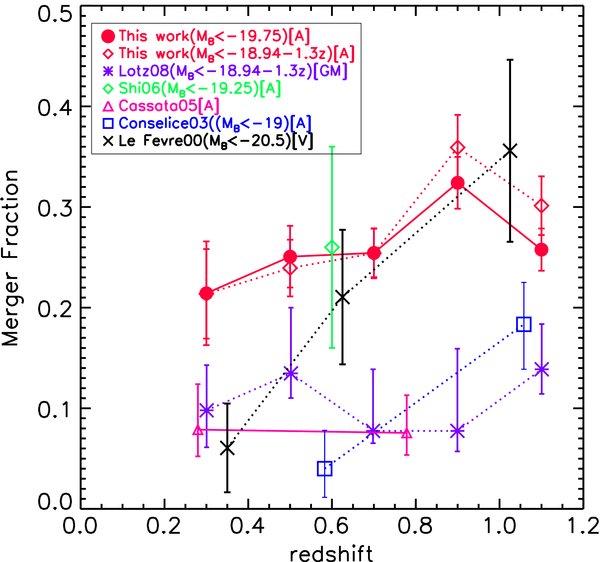
Figure 7. Redshift evolution of galaxy merger fractions with given B-band magnitude cuts. A: mergers identified with asymmetry; GM: Gini-M20 classified mergers; V: visually classified mergers.
Download figure:
Standard image High-resolution imageWe notice that our relatively high merger fraction (20%) at z = 0.2–0.4 may require a rapid evolution to that at z = 0. However, the current understanding of the galaxy merger fraction at z < 0.2 is much less constrained mainly due to the small volume and use of shallow images with poor spatial resolution. For example, De Propris et al. (2007) measured a merger fraction with asymmetry for a complete galaxy sample from the Millennium Galaxy Catalog (MGC) and found a merger fraction of 2%–4% depending on the definition of possible contaminators. However, the poor spatial resolution (1.3 arcsec) and shallow exposure (sky noise = 26 mag arcsec−2) of the MGC survey (Cross et al. 2004), provide rest-frame B-band image quality for galaxies at z = 0.1 only comparable to z = 1 galaxies observed in the GOODS survey, implying a possibly significant underestimate of the merger fraction due to SB effects. The image quality is even worse for the SDSS and 2dFGRS images. Current HST data do not provide a statistically large complete galaxy sample at z < 0.2. The fraction of mergers identified as galaxy pairs is also not well constrained, from 1% (De Propris et al. 2007) to 5% (Lin et al. 2008) for the same set of data but with different methods, which again suggests that more thorough studies are required to have good constraints on galaxy mergers at z < 0.2.
4.4. Infrared and B-Band Luminosity Functions of Galaxy Mergers
4.4.1. Methodology for Constructing IR Luminosity Function
The IR LFs of galaxy mergers are derived broadly following the works of Le Floc'h et al. (2005) and Shi et al. (2008). The 1/Vmax method (Schmidt 1968) is applied to galaxy mergers with mz< 25, f24 μm > 60 μJy and known redshifts. The comoving number density in a given luminosity bin can be written as

where ω is the weight to correct for incompleteness and Vmax is the maximum volume for an object to be included in the sample. Vmax is given by
where [zlow, zhigh] is the redshift over which the object can be detected and Ω is the survey solid angle (730 arcmin2). Note that the field edge excluded for the morphology study is a small fraction (1%) of the total area. While zlow is always fixed to the low end of a redshift interval, the maximum redshift, zhigh, is defined as
where zhighbin is the high end of a redshift interval and zlimitIR is the limiting redshift at which the observed IR flux reaches the limiting flux of 60 μJy. The K-correction for 24 μm flux is based on the star-forming templates of Rieke et al. (2009).  is the limiting redshift where the observed z-band magnitude reaches mlimitz = 25. The K-correction in the z band is based on the ACS photometry and KCORRECT code (Blanton et al. 2003; Blanton & Roweis 2007).
The incompleteness correction ω includes corrections for the IR detection, IR objects associated with optical counterparts at mz < 25, the redshift measurement success rate, and the criterion of secure morphologies. The incompleteness of the IR detections as a function of the 24 μm flux density is given in Papovich et al. (2004). Our sample is limited to f24 μm = 60 μJy at which the incompleteness is ∼50%. There is no incompleteness correction for IR objects associated with optical counterparts with mz< 25. This is because mz< 25 is deep enough to detect nearly all optical counterparts of the IR objects brighter than f24 μm = 60 μJy, given the rough correlation between the IR luminosity and optical luminosity in Le Floc'h et al. (2005). The incompleteness correction for redshift measurements is defined as the ratio of the number of all objects to that of objects with redshift measurements within a three-dimensional magnitude–color–color space mz–(B − i)–(V − z). Such corrections can account for redshift measurement success as a function of the galaxy brightness and color. For the whole ACS photometry sample at mz< 25, the success rate for redshift measurements is 68%. The final correction is for galaxies with secure morphologies, i.e., galaxy radius Rgal > 15 pixel and asymmetry uncertainty error(A) < 0.1. Such a correction is defined as the ratio of the number of all objects to that of objects with secure morphologies within a given luminosity bin and a given redshift bin. Note that these corrections are small (less than 1.2) except for the highest luminosity bin in 0.4 <z< 0.6 (a correction factor of 1.5). This indicates that the final IR LF of galaxy mergers is mainly based on objects with secure morphologies.
4.4.2. IR Luminosity Function of Galaxy Mergers
Figure 8 shows the IR LFs of galaxy mergers within different redshift bins. As shown in the figure, our IR LFs of field galaxies match those of Le Floc'h et al. (2005) well. The 1σ uncertainties of the IR LFs of galaxy mergers include the Poisson noise, the uncertainty in the 24 μm-to-LIR conversion and cosmic variance. Since our field size is almost as large as that in Le Floc'h et al. (2005) and 24 μm flux density is used to derive the total IR luminosity in both works, for the uncertainty in the 24 μm-to-LIR conversion and cosmic variance, we simply adopted the result obtained by Le Floc'h et al. (2005), an average of 0.2 dex upper side uncertainty and 0.1 dex lower side uncertainty. The final uncertainty including the Poisson noise is plotted in Figure 8 and listed in Table 2. The solid lines are the fit to the IR LFs of field galaxies while the dotted lines are the fit to the IR LFs of galaxy mergers. The curve for the fit is the Schetcher function. Although the Schetcher function fails to fit the local field galaxy IR LF (Pérez-González et al. 2005), our limited available data points do not allow us to use a formula with more parameters, such as a double power law. The slope of the Schetcher function is fixed as the average value of the fit to the IR LFs in the first two redshift bins. The fitted result is listed in Table 3.
Figure 8. Infrared luminosity functions of galaxy mergers at different redshifts (open stars), where upper and lower limits at a given IR luminosity correspond to the result with asymmetry corrections based on redshifted local LIRGs and redshifted low-z GOODS galaxies for galaxies with LIR > 2.5 ×10¹¹ L☉, respectively, while asymmetry corrections based on redshifed low-z GOODS galaxies are used for galaxies with lower IR luminosity. The open circles are the infrared luminosity function of GOODS field galaxies. The gray area shows the luminosity function and 3σ uncertainty of field galaxies obtained by Le Floc'h et al. (2005). The dotted line is the fit to the IR LF of galaxy mergers, while the solid line is the fit to the IR LFs of general field galaxies. The merger fraction as a function of the IR luminosity is also shown.
Download figure:
Standard image High-resolution imageTable 2. Infrared Luminosity Function of Merger Galaxies
| Φ (h370 Mpc−3 Log L−1☉) | ||||
|---|---|---|---|---|
| Log(LIR (h−270 L☉)) | 0.4 <z< 0.6 | 0.6 <z< 0.8 | 0.8 <z< 1.0 | 1.0 <z< 1.2 |
| 10.75a | (4.60+2.27−1.33) ×10−4 | ... | ... | ... |
| 11.25a | (3.05+1.55−0.96) ×10−4 | (3.64+1.77−1.01) ×10−4 | (5.66+2.69−1.45) ×10−4 | (6.26+3.28−2.13) ×10−4 |
| 11.75a | (4.23+3.11−2.61) ×10−5 | (1.83+0.93−0.58) ×10−4 | (4.40+2.10−1.15) ×10−4 | (5.58+2.63−1.41) ×10−4 |
| 12.25a | ... | (1.56+1.38−1.23) ×10−5 | (1.07+0.56−0.37) ×10−4 | (1.95+0.96−0.56) ×10−4 |
| 12.75a | ... | ... | ... | (2.90+1.85−1.44) ×10−5 |
| 10.75b | (4.60+2.27−1.33) ×10−4 | ... | ... | ... |
| 11.25b | (3.06+1.55−0.96) ×10−4 | (3.54+1.72−0.99) ×10−4 | (5.14+2.44−1.33) ×10−4 | (5.85+3.11−2.06) ×10−4 |
| 11.75b | (4.22+3.10−2.61) ×10−5 | (1.40+0.73−0.48) ×10−4 | (2.74+1.33−0.76) ×10−4 | (2.73+1.32−0.75) ×10−4 |
| 12.25b | ... | (1.12+1.12−1.03) ×10−5 | (7.11+3.94−2.74) ×10−5 | (1.11+0.57−0.36) ×10−4 |
| 12.75b | ... | ... | ... | (1.73+1.27−1.06) ×10−5 |
Notes. aThe galaxy asymmetries are corrected based on the redshifted local LIRGs. bThe galaxy asymmetries are corrected based on the redshifted low-z (z= 0.2–0.4) GOODS field galaxies.
Download table as: ASCIITypeset image
Table 3. Parameters of Schetcher Function Fit to IR LFs of Galaxy Mergers
| Redshift | Log(Φ*) (h370 Mpc−3 Log L−1☉) | Log(L*) (h−270 L☉) | α |
|---|---|---|---|
| 0.4 < za<0.6 | −3.63+0.06−0.05 | 11.37+0.08−0.03 | −1.12+0.00−0.00 |
| 0.6 < za<0.8 | −3.70+0.06−0.10 | 11.75+0.07−0.00 | −1.12+0.00−0.00 |
| 0.8 < za<1.0 | −3.59+0.09−0.03 | 12.04+0.17−0.00 | −1.12+0.00−0.00 |
| 1.0 < za<1.2 | −3.62+0.02−0.03 | 12.29+0.04−0.06 | −1.12+0.00−0.00 |
| 0.4 < zb<0.6 | −3.63+0.06−0.05 | 11.37+0.08−0.04 | −1.12+0.00−0.00 |
| 0.6 < zb<0.8 | −3.72+0.07−0.11 | 11.70+0.07−0.01 | −1.12+0.00−0.00 |
| 0.8 < zb<1.0 | −3.67+0.04−0.04 | 11.98+0.13−0.04 | −1.12+0.00−0.00 |
| 1.0 < zb<1.2 | −3.80+0.02−0.08 | 12.26+0.03−0.07 | −1.12+0.00−0.00 |
Notes. aThe galaxy asymmetries are corrected based on the redshifted local LIRGs. bThe galaxy asymmetries are corrected based on the redshifted low-z (z= 0.2–0.4) GOODS field galaxies.
Download table as: ASCIITypeset image
Figure 8 also shows the fraction of galaxy mergers as a function of the IR luminosity in different redshift bins. At all redshifts, the merger fraction increases with the IR luminosity, a trend similar to that for local galaxies (Sanders & Mirabel 1996).
4.4.3. B-Band Luminosity Function of Galaxy Mergers
The rest-frame B-band LFs of galaxy mergers are also derived as shown in Figure 9. The result of the merger B-band LF is listed in Table 4. Again, Schetcher functions are used to fit the data points where the slope is fixed as the average value of the fit to the LF in the first three redshift bins. The fitted result is listed in Table 5. For the B-band LFs, there are enough data points to break the luminosity–density degeneracy. The result is shown in Figure 10. For the general field B-band LF, Φ* ∝ (1 + z)0.1±0.5 and ΔM*B ∝ (−0.4 ± 0.3)Δz, which are generally consistent with the literature data (see Faber et al. 2007, and references therein). For the merger B-band LF, Φ* ∝ (1 + z)0.5±0.5 and ΔM*B ∝ (−0.4 ± 0.3)Δz.

Figure 9. B-band luminosity functions of galaxy mergers (open stars) and general field galaxies (open circles) at different redshifts. The dotted line is the fit to the LF of galaxy mergers while the solid line is the fit to that of general field galaxies.
Download figure:
Standard image High-resolution imageTable 4. B-Band Luminosity Function of Merger Galaxies
| Φ (h370 Mpc−3 Log L−1☉) | |||||
|---|---|---|---|---|---|
| MB | 0.2 <z< 0.4 | 0.4 <z< 0.6 | 0.6 <z< 0.8 | 0.8 <z< 1.0 | 1.0 <z< 1.2 |
| −22.40 | ... | ... | (6.18+2.34−2.34) ×10−5 | (3.09+1.34−1.34) ×10−5 | (3.93+1.48−1.48) ×10−5 |
| −21.60 | (1.28+0.58−0.58) ×10−4 | (9.19+3.53−3.53) ×10−5 | (1.84+0.53−0.53) ×10−4 | (1.71+0.48−0.48) ×10−4 | (2.04+0.54−0.54) ×10−4 |
| −20.80 | (1.68+0.69−0.69) ×10−4 | (3.31+0.93−0.93) ×10−4 | (3.61+0.94−0.94) ×10−4 | (4.34+1.09−1.09) ×10−4 | (2.98+0.76−0.76) ×10−4 |
| −20.00 | (3.48+1.14−1.14) ×10−4 | (4.87+1.30−1.30) ×10−4 | (4.17+1.07−1.07) ×10−4 | (5.74+1.41−1.41) ×10−4 | (3.37+0.85−0.85) ×10−4 |
| −19.20 | (2.04+0.78−0.78) ×10−4 | (3.19+0.90−0.90) ×10−4 | (3.42+0.90−0.90) ×10−4 | (4.42+1.11−1.11) ×10−4 | ... |
| −18.40 | (2.88+0.99−0.99) ×10−4 | (2.48+0.74−0.74) ×10−4 | (3.10+0.82−0.82) ×10−4 | ... | ... |
| −17.60 | (1.93+0.75−0.75) ×10−4 | (1.92+0.60−0.60) ×10−4 | ... | ... | ... |
| −16.80 | (1.07+0.51−0.51) ×10−4 | ... | ... | ... | ... |
Download table as: ASCIITypeset image
Table 5. Parameters of Schetcher Function Fit to Merger B-band LFs
| Redshift | Log(Φ0*) (h370 Mpc−3 M−1B) | M0B* | α |
|---|---|---|---|
| 0.2 < z<0.4 | −3.52+0.00−0.05 | −20.72+−0.03−0.13 | −0.53+0.00−0.00 |
| 0.4 < z<0.6 | −3.43+0.05−0.01 | −20.63+−0.11−0.01 | −0.53+0.00−0.00 |
| 0.6 < z<0.8 | −3.39+0.04−0.03 | −21.05+−0.08−0.00 | −0.53+0.00−0.00 |
| 0.8 < z<1.0 | −3.29+0.02−0.02 | −20.77+−0.01−0.06 | −0.53+0.00−0.00 |
| 1.0 < z<1.2 | −3.47+0.05−0.02 | −21.04+−0.02−0.03 | −0.53+0.00−0.00 |
Download table as: ASCIITypeset image
Figure 10. Evolution in the luminosity and density of B-band luminosity functions of galaxy mergers (diamonds) and general field galaxies (triangles).
Download figure:
Standard image High-resolution imageThe breaking of the luminosity–density degeneracy allows us to evaluate the evolution of the pure merger fraction:

Given ngalaxy ∝ (1 + z)0.1±0.5 and nmerger ∝ (1 + z)0.5±0.5 in the B band, we have
The weak redshift evolution of the pure merger fraction fBmerger indicates that the observed weak evolution in a given B-band magnitude is really caused by the weak evolution of the galaxy merger number density relative to the total number density. The merger rate can be estimated through the merger fraction and the timescale of 0.2–1.1 Gyr over which the asymmetry parameter can identify mergers (Lotz et al. 2008b).
5. DISCUSSION
5.1. Merger-Dominated High-Redshift LIRG Morphologies and High Merger Fractions in General Field Galaxies
While the local LIRGs are dominated by mergers (Sanders & Mirabel 1996), the result for high-redshift LIRGs is controversial, with merger fractions from as low as 10%–20% (Zheng et al. 2004; Bell et al. 2005; Bridge et al. 2007; Lotz et al. 2008a; Melbourne et al. 2008) to ∼50% (Shi et al. 2006). Motivated by the result of Shi et al. (2006) in the UDF field, we re-evaluated the effect of SB dimming on the morphology measurements. We first revised the asymmetry measurement based on simulations. Our new method shows a smaller scatter and does not suffer from a systematic offset compared to the one in the literature. We then obtained redshift-, IR-luminosity- and optical-luminosity-dependent asymmetry corrections by measuring asymmetry deficits of local LIRGs and low-z GOODS galaxies redshifted to different higher redshifts. By applying these corrections, we have found that high-redshift LIRGs are generally highly asymmetric galaxies with implied merger fractions ∼50% up to z= 1.2. For the general galaxy population, we obtained a weak evolution of merger fractions, consistent with results of Bundy et al. (2004), Lin et al. (2008), Lotz et al. (2008a), and de Ravel et al. (2008), but with several times higher merger fractions (20%–30%).
In Sections 4.2 and 4.3, we summarized possible reasons for the lower fractions of morphologically identified mergers in other studies (Le Fèvre et al. 2000; Zheng et al. 2004; Conselice et al. 2003; Cassata et al. 2005; Bell et al. 2005; Bridge et al. 2007; Lotz et al. 2008a; Melbourne et al. 2008).
The low fraction of kinematic galaxy pairs (Le Fèvre et al. 2000; Lin et al. 2008; de Ravel et al. 2008) is at least partly due to the different timescales probed by this method compared to morphology studies. Also, kinematic pairs are exclusively major mergers while a small fraction of highly asymmetric objects may be minor mergers. Our high merger fraction is consistent with the incidence of mergers identified through disturbed velocity fields. Specifically, studies of the velocity fields of ∼60 galaxies at 0.4 <z< 0.75 (Neichel et al. 2008; Yang et al. 2008) find a low fraction of rotationally supported disk galaxies and high fraction (41% ± 7%) of galaxies with complex kinematics. Neichel et al. (2008) also show that the auto classifications (CA and Gini-M20 without corrections) miss half of the galaxies with complex kinematics and misclassify them as normal disk galaxies (also see a similar result from numerical simulations; Lotz et al. 2008b).
5.2. Contribution by Galaxy Mergers to the Cosmic IR Energy Density
We have derived IR LFs of galaxy mergers at different redshifts out to z= 1.2. With these IR LFs, we now can quantitatively evaluate the contribution of galaxy mergers to the cosmic IR energy density out to z∼ 1.2. The open circle in the top panel of Figure 11 shows the cosmic IR energy density estimated by integrating general IR LFs obtained in this work, compared to the work of Pérez-González et al. (2005; gray area). The open star is the evolution of the cosmic IR energy density of galaxy mergers obtained by integrating the IR LFs of galaxy mergers where the upper and lower limits correspond to the result with asymmetry corrections based on redshifted local LIRGs and low-z GOODS field galaxies, respectively. The bottom panel of the figure shows the ratio of the merger IR energy density to the total IR energy density.
Figure 11. Top panel: the total cosmic IR density (open circles) compared to the result (gray area) of Pérez-González et al. (2005). The open star symbols are the upper and lower limits of the cosmic IR density with 1σ uncertainty contributed by galaxy mergers (see Figure 8). Bottom panel: the ratio and 1σ uncertainty of the merger IR density to the total IR density.
Download figure:
Standard image High-resolution imageThe galaxy mergers-produced IR energy density shows dramatic evolution: ΩmergersIR∝ (1+z)∼5 and (1+z)∼6 for the result with low and high asymmetry corrections, respectively, compared to the total IR energy density evolution (1+z)3.0 (Le Floc'h et al. 2005; Pérez-González et al. 2005). At z ≳ 1, the cosmic IR energy density is dominated by galaxy mergers. This result can be expected since LIRGs dominate the IR energy density at z > 0.7 (Le Floc'h et al. 2005; Pérez-González et al. 2005) and LIRGs are dominated by galaxy mergers, as found in this work.
To convert the cosmic energy IR density to the cosmic SFR density, the unobscured star formation as traced by the UV energy density needs to be included. In the local universe, the UV energy density corresponds to about 30% of the cosmic SFR density and decreases to 10% at z = 1.2 (Le Floc'h et al. 2005). The indicated correction from the cosmic IR energy density to the total SFR density for nonmergers should be larger than those for mergers, as the merger IR energy density has contributions from galaxies with on-average higher IR luminosity. This implies that Figure 11 may overestimate the contribution of galaxy mergers to the total cosmic SFR density.
6. CONCLUSIONS
We present detailed morphology studies of intermediate-redshift (0.2 < z<1.2) LIRGs and general field galaxies in the GOODS field by measuring galaxy concentration and asymmetry, with the goal to constrain the role of galaxy mergers in the cosmic SFH. Our main conclusions are as follows.
- 1.A new asymmetry determination method is proposed to account for the importance of underlying background structures in accurate asymmetry measurements. Simulations indicate that our method does not suffer from a systematic offset and has small intrinsic uncertainty.
- 2.The redshift dependence of the galaxy asymmetry due to SB dimming is a function of the asymmetry itself, with larger corrections for more asymmetric objects. This requires careful asymmetry corrections for high-redshift galaxies.
- 3.With the necessary asymmetry corrections, high-redshift LIRGs are generally galaxies with high asymmetries and have implied merger fractions of ∼50% up to z = 1.2, although they are slightly more symmetric than local LIRGs.
- 4.With similar asymmetry corrections, high-redshift general field galaxies show a weak redshift evolution of merger fractions up to z= 1.2 but with a relatively high merger fraction (20%–30%).
- 5.The B-band LFs of galaxy mergers show evolution in the luminosity and density similar to general field galaxies. By removing the luminosity–density degeneracy, the pure number density of galaxy mergers relative to the total density shows weak redshift evolution, i.e., (1 + z)m with m = 0.4 ± 0.7.
- 6.The IR LF s of galaxy mergers are derived in several redshift bins: they indicate that the merger fraction increases with the IR luminosity. The integral of these LFs shows that the cosmic IR energy density from galaxy mergers shows a dramatic redshift evolution ((1 + z)∼5−6) and starts to dominate the total cosmic IR energy density at z≳1.
Our study has been confined to the CA method of morphology determination. The significant corrections we derive for this method indicate that a similar study of other methods (e.g., Gini-M20) would be desirable.
We thank the anonymous referee for detailed comments. Support for this work was provided by NASA through contract 1255094 issued by JPL/California Institute of Technology. J.M.L. acknowledges support from Leo Goldberg Fellowship sponsored by the National Optical Astronomy Observatory. P.G.P.-G. acknowledges support from the Spanish Programa Nacional de Astronomía y Astrofísica under grants AYA 2006–02358 and AYA 2006–15698–C02–02, and from the Ramón y Cajal Program financed by the Spanish Government and the European Union.
APPENDIX A: NEW NOISE CORRECTION
We revisit here the problem of the sky noise asymmetry correction. In the case of high-redshift galaxies, we find that using the minimum-noise asymmetry to correct the min(Agalaxy+noise), as proposed by Conselice et al. (2000), overestimates the true galaxy asymmetry and results in a relatively large error.
The noise correction is critical for an accurate measurement of the true galaxy asymmetry. For example, even for the minimum-noise asymmetry correction (i.e., Acorrnoise = min(Anoise), referred to as the minimum method in the following), Acorrnoise is a significant fraction of Agalaxy+noise. The median value of min(Anoise)/Agalaxy+noise reaches almost 70% for the local relatively high-SB galaxy sample from Frei et al. (1996), which Conselice et al. (2000) used as a test sample for the asymmetry parameter. We have used the GOODS-S field and the UDF to test ways to measure asymmetry. We carried out a simulation to optimize the estimate of the true Acorrnoise underlying min(Agalaxy+noise), using noise asymmetries measured in fields placed randomly around the galaxy. The basic idea of the simulation is illustrated in Figure 12. A UDF galaxy image was superposed on a clean GOODS background region to create an artificial GOODS galaxy. For this galaxy, the galaxy size, concentration, and the rotation centers giving min(Agalaxy+noise) were measured. The resulting rotation center and galaxy size were then used with the galaxy removed to measure the asymmetry of the clean GOODS background region, which should give the true Acorrnoise. By putting circular regions with the same aperture size randomly on this background region, the randomly produced noise asymmetry distribution was obtained. The goal was to find the best way to use the randomly produced noise asymmetry distribution to estimate the true Acorrnoise. In this experiment, the direct measurements of the true noise correction values let us test our method.
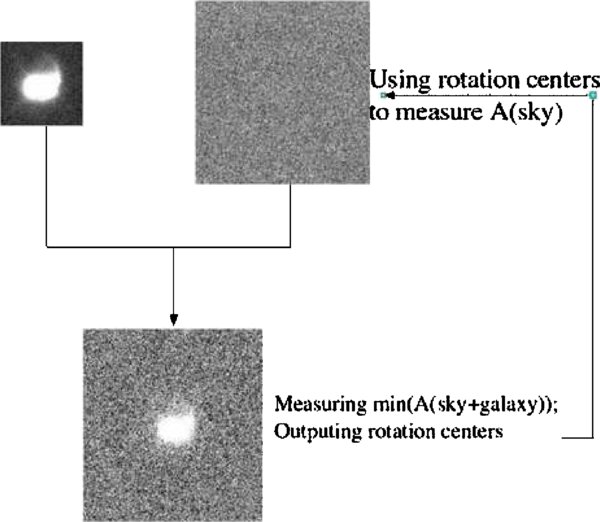
Figure 12. Illustration of the basic idea for finding the real noise correction for min(Agalaxy+noise). A UDF galaxy image is superposed on a clean GOODS background region to create an artificial GOODS galaxy. For this galaxy, the galaxy size, concentration, and the rotation centers giving min(Agalaxy+noise) can be measured. The resulting rotation centers and galaxy size are then used to measure the asymmetry of the clean GOODS background region, which should give the real noise correction for min(Agalaxy+noise).
Download figure:
Standard image High-resolution imageHere we describe the details of the simulation. First, we used the GOODS-S z-band catalog to select a total of 13 clean z-band GOODS background regions with sizes of 400 × 400 pixels (1 pixel = 003). As the GOODS catalog only indicates if the galaxy center is outside the region or not, we inspected each region to make sure there was no extended emission from galaxies with centers outside the region. These regions were distributed over the whole field to account for any variations over the field. We then picked 25 UDF galaxies spanning a range of S/N (50–1000) within half radii. The main reason for using UDF galaxies is that the UDF is deep enough to detect faint asymmetric structures. Our test will thus not be biased by low S/N. The UDF segmentation images were used to define the galaxy pixels. These galaxy pixels were superposed on each of the 13 GOODS background regions. For each UDF galaxy and GOODS background region, 121 artificial images were created by putting the UDF galaxy at each position of an 11 × 11 grid with a separation of 10 pixels over the central 100 × 100 pixel regions of the GOODS background image. For these 121 artificial images, we measured the galaxy size and true noise asymmetry correction as described in the above paragraph. We then used the mean size of these galaxies to produce the distribution of random noise asymmetry corrections by putting circular regions randomly within the GOODS background image. Based on these randomly produced corrections within the average aperture, we created 1000 random corrections for each artificial galaxy by multiplying the corrections within the average aperture with the aperture size (area) of the artificial galaxy relative to the average aperture size (Conselice et al. 2000). In summary, for one UDF galaxy and one GOODS background image, we have 121 true noise asymmetry corrections corresponding to 121 artificial galaxies and for each artificial galaxy we have a distribution of 1000 randomly produced noise asymmetry measures. Note that the noise associated with the UDF galaxy itself is not an issue in this experiment, as any noise pattern associated with the UDF galaxy acts like the galaxy signal in terms of searching for rotation centers giving min(Agalaxy+noise).
Figure 13 shows comparisons between the true noise asymmetry corrections (dotted line; 121 asymmetry values in each panel) and the randomly produced noise asymmetry (solid line; 121 × 1000 asymmetry values in each panel) for the 13 clean GOODS sky regions superposed with a high-S/N (∼1000) UDF galaxy, while Figure 14 shows result for a low-S/N (∼70) UDF galaxy. The vertical line indicates the median value of each distribution. Figures 13 and 14 indicate that using the minimum-noise asymmetry to correct the noise asymmetry underlying min(Agalaxy+noise) will overestimate the real galaxy asymmetry in many cases. The true sky asymmetry correction actually lies approximately between two extreme cases, the minimum value and the median of the randomly produced noise asymmetry. The minimum case is reached when the galaxy is so faint that the min(Agalaxy+noise) is actually dominated by the background. The median correction is appropriate when the galaxy is so bright that the min(Agalaxy+noise) is dominated by galaxy signal, as shown in Figure 13. Because we usually apply a lower limit S/N cut, we will rarely have the former case. A more important implication from these two figures is that the backgrounds always have unknown structures, which makes accurate noise correction impossible. Even for the same UDF galaxy and the same GOODS background image, the scatter of the true noise asymmetry correction is significant. For a high-S/N (1000) UDF galaxy as shown in Figure 13, the scatter is about 20% (or σ(A)= 0.02) and it reaches 50% (or σ(A)= 0.2) for a low-S/N (70) UDF galaxy as shown in Figure 14. The difference in the true correction between different GOODS background regions superposed with the same UDF galaxy is also nonnegligible. The fluctuation in the background can be caused by nonuniform exposure, variation in the detector response, Poisson noise and probably more important for the deep survey, a large number of objects below the detection limit.
Figure 13. Comparisons between the true noise asymmetry corrections (dotted line; 121 asymmetry values in each panel) and the randomly produced noise asymmetry (solid line; 121 × 1000 asymmetry values in each panel) for 13 clean GOODS background regions superposed with a high-S/N (∼1000) UDF galaxy. The vertical lines are the median values of two distributions.
Download figure:
Standard image High-resolution image
Figure 14. Same as in Figure 13 but for a low-S/N (70) UDF galaxy.
Download figure:
Standard image High-resolution imageGiven the significant scatter in the true noise correction caused by complicated background structures and the fact that we can only measure the noise asymmetry in the background region around (instead of underlying) the galaxy, we tried to find the best way to use the randomly produced noise corrections to estimate the true value. To do this, we measured the fraction of the randomly produced corrections below the true value for each artificial galaxy. The median value of the distribution of this fraction is 0.15. Therefore, the value at the 15% probability low-end tail of the randomly produced noise corrections gives the best estimate of the true value. Figure 15 compares our new noise correction (described as the 15% probability method in the following) to the minimum method where the minimum correction is simply the minimum of the randomly produced corrections. As shown in Figure 15, the minimum-noise-corrected galaxy asymmetry overestimates the true value, with a median offset of δA = −0.05. It may not be a severe problem to use the minimum-noise correction as long as all the morphologies are measured in the same way. However, we emphasize that, as discussed above and shown in Figures 13–15, it is impossible to recover an accurate noise correction due to the complicated background structures. Figure 15 indicates that the 68% confidence range of Acorrnoise–Arealnoise of our method is 0.044 compared to 0.074 for the minimum method. A scatter of 0.074 is actually quite large given the merging criteria of A > 0.35 for the minimum method (Conselice et al. 2003). Our 15% probability method provides almost two times less scatter in the Acorrnoise–Arealnoise compared to the minimum method.

Figure 15. Solid histogram shows the difference between the noise correction of our 15% probability method and the true correction, while the dotted one shows the difference between the correction of the minimum method and the true correction. The vertical lines indicate the 16% and 84% low-end probability tail of these two histograms. The median offsets of our method and the minimum one are 0.00 and −0.05, respectively. The 68% confidence range of our method and minimum one are 0.044 and 0.074, respectively.
Download figure:
Standard image High-resolution imageFigure 16 shows the difference (σrealnoise = |A15%noise − Arealnoise|) between the true correction and our 15% probability method as a function of the standard deviation (σrandomnoise) of the randomly produced noise corrections. As shown above, the noise corrections are affected by unknown background structures and thus it would be expected that there is no correlation between σrealnoise and σrandomnoise. However, the maximum σrealnoise for a given σrandomnoise is roughly correlated with σrandomnoise. As shown by the solid line, 2 ×σrandomnoise should give an upper limit to σrealnoise valid for 99% of the objects in the simulation (e.g., effectively at about 3σ significance).

Figure 16. Difference (σrealnoise = |A15%noise − Arealnoise|) between the true correction and our 15% probability method as the function of the standard deviation (σrandomnoise) of the randomly produced noise corrections. The solid line shows σrealnoise= 2σrandomnoise which can be used to provide conservative estimate of σrealnoise for the 99% objects in the simulation.
Download figure:
Standard image High-resolution imageAs a summary, we propose a new noise asymmetry correction. A set of 1000 randomly produced noise corrections is produced by putting circular regions in the background image around the target. The value of this distribution at the 15% probability low-end tail is used to correct the noise asymmetry for min(Agalaxy+noise). The error (∼3σ) in the final measured galaxy asymmetry is taken to be two times the standard deviation of these randomly produced noise asymmetries. In reality, some galaxies are always present in the field of targets. To account for this problem, we defined the success rate for the 1000 circular region placements as the fraction of circular regions containing no galaxy signal indicated by the SExtractor segmentation image. Circular regions containing any galaxy signal were not used. More sets of 1000 placements were done until 1000 successful measurements were reached. If the success rate for one set of placements is lower than 50%, the circular region size for the following set is taken to be 80% of this set. Then, the measured background asymmetry is rescaled to that with the original size by assuming background asymmetry proportional to the aperture area (Conselice et al. 2000).
APPENDIX B: MORPHOLOGIES OF REDSHIFTED LOCAL LIRGS AND LOW-z GOODS FIELD GALAXIES
B.1. Morphologies of Redshifted Local LIRGs
The B-band morphologies of the local LIRGs at LIR > 1011.4 L☉ were measured following the procedure described in Section 2.2. Due to the high resolution and the nature of complicated morphologies, about 10% of the local LIRGs have multiple radii at η(r)= 0.2. For these objects, we used the maximum radius at η(r)= 0.2 that matches the visually identified galaxy size well.
To account for the redshift dependence of LIRG morphologies, we also measured the redshifted B-band morphologies of these LIRGs at redshifts of 0.5, 0.7, 0.9, and 1.1. Since we quantified the GOODS galaxy morphologies using the rest-frame B-band images, we put the local LIRGs into a clean GOODS V-band sky region for local LIRGs redshifted to z = 0.5, i-band sky region for redshifted LIRGs at z = 0.7 and z = 0.9, and z-band sky region for redshifted LIRGs at z = 1.1. The exposure times for GOODS V-, i-, and z-band images are around 5000, 7000, and 20,000 s, respectively. The clean GOODS sky region has a size of 24'' × 24'', which is large enough to cover very extended tidal tails. The GOODS field is too crowded to have a continuous 24'' × 24'' clean region without any intruding object. Our field is obtained by merging four 12'' × 12'' clean regions whose sky fluctuations are consistent with each other within 3%.
To redshift the LIRGs, the pixel size was rebinned through IDL FREBIN.pro which rebins the pixel assuming the flux within a pixel is constant over the pixel area. We did not apply any size evolution, since on average the galaxy size Rp of LIRGs does not change with redshift. The DN per second of the local LIRG B-band images was converted to the GOODS ACS counts at a given band by using their PHOTOFLAM values and then decreased by the square of the luminosity distance and (1 + z), where (1 + z) is the K-correction, since PHOTOFLAM is defined as inverse sensitivity in units of erg cm−2 s−1 Å−1. The resulting DN per second is then brightened by 0.60z magnitudes, which accounts for the redshift dependence of the rest-frame B-band magnitude of LIRGs as shown in Figure 17.
Figure 17. Redshift evolution of the B-band magnitude of LIRGs with LIR > 1011.4 L☉, where the z = 0 point is for local LIRGs and higher redshift points are for LIRGs in GOODS. The diamonds with error bars show the median values and 68% confidence ranges of the B-band magnitude distribution at z = 0, 0.4 <z < 0.6, 0.6 < z < 0.8, 0.8 < z < 1.0 and 1.0 < z<1.2. The solid line gives the linear fit mB = −20.53 − 0.60z.
Download figure:
Standard image High-resolution imageDuring this pixel-rebinned and flux-rescaled process, the original LIRG image noise was correspondingly scaled down. To mimic the galaxy morphologies measured in the real GOODS sky region, the original galaxy background fluctuation should not dominate over the GOODS background in measuring the redshifted local LIRGs. To quantify when the scaled original galaxy background does not affect the redshifted LIRG morphology measurement, we carried out a test to measure the asymmetry of a clean GOODS sky region superposed on a second GOODS sky region scaled down by a given factor. When the second sky region has a scaled-down factor of <0.3, its effect on the asymmetry measurements of the first sky region is negligible. Therefore, we measured all redshifted LIRGs with rescaled original background noise smaller than 0.3 of the GOODS sky noise. At redshifts of 0.5, 0.7, 0.9, and 1.1, the numbers of measurable redshifted LIRGs are 61, 83, 88, and 88 out of a total of 88 local LIRGs. Therefore, the redshifted LIRGs are still representative of the complete local LIRG sample.
B.2. Morphologies of Redshifted Low-z Field Galaxies
The galaxy sample that we used is the V-band images of 596 GOODS galaxies at 0.2 <z< 0.4 with secure morphology measurements. For a fiducial galaxy at z = 0.3, the GOODS V-band exposure corresponds to a 10σ rest-frame B-band SB of 25.5 mag arcsec−2, comparable to the depth of the HST observations of local LIRGs (25.0 mag arcsec−2). The algorithm to measure morphologies of redshifted galaxies is almost the same as for redshifted local ULIRGs with two differences. First, we did not require the rescaled original galaxy noise to be <0.3 times the noise in the band where galaxies are redshifted to. Instead, we used the following strategy:

where Inew is the final new image, Iold is the rebinned and rescaled original galaxy, Bnew is the new background image in the band where the galaxy is redshifted to, and η is the ratio of rescaled and rebinned original galaxy noise to the fluctuation in Bnew. This method will make sure that all redshifted galaxies will be used at all redshifts while maintaining the noise level. The main reason that we did not use this method for local LIRGs is that we wanted to quantify the effect of the complicated background structures in deep fields on the asymmetry measurements.
Second, no additional B-band luminosity evolution is applied, although there is a luminosity evolution in the B-band LF (e.g., Faber et al. 2007). This is because, ideally, the asymmetry correction for a distant galaxy should be based on the asymmetry deficit of a redshifted low-z galaxy with intrinsically the same asymmetry and B-band brightness. Applying B-band luminosity evolution will artificially underestimate the effect of SB dimming. To further demonstrate this argument, we measured the asymmetry deficits for redshifted galaxies with B-band luminosity evolution (ΔMB = −1.1Δz; Faber et al. 2007) and no evolution. This result can be compared to the real result obtained by comparing the asymmetries using GOODS images and UDF images for the same galaxies. The result is shown in Figure 18 for galaxies with 0.4 < z<0.8 within which range the UDF limiting SB in the z-band is comparable to the GOODS v-band limiting SB at z= 0.3. As indicated by the figure, the cases with evolution underestimate the asymmetry correction significantly.

Figure 18. Asymmetry deficit vs. intrinsic asymmetry. The open circles and stars are for low-redshift (0.2 < z < 0.4) GOODS galaxies redshifted to 0.4 < z < 0.8 with B-band luminosity evolution and no evolution, respectively. The diamonds show the evolution-independent result, which is the asymmetry difference using GOODS images (low S/N) and UDF images (high S/N) for galaxies with 0.4 < z < 0.8. The error bars are given at the 16% and 84% probability limits.
Download figure:
Standard image High-resolution imageB.3. The Asymmetry Deficit due to SB Dimming is a Function of the Asymmetry Itself
Figure 19 shows the median asymmetries and the 68% confidence ranges for the local LIRGs and redshifted local LIRGs at z = 0.5, 0.7, 0.9, and 1.1. The exposure time at each redshift is labeled. As shown in the figure, the galaxy appears more symmetric at high redshifts as more low-SB asymmetric structures are embedded in the background fluctuations due to SB dimming. A linear fit to central three points with similar exposure times (∼6000 s) gives δA/δz = −0.38. The asymmetry of the local LIRGs is below the extrapolation of this linear fit as the local LIRGs should be more asymmetric at the exposure time of ∼6000 s. The redshifted LIRGs at z = 1.1 are above the extrapolation of this fit as a deeper exposure at z band detects more faint asymmetric structures. Although the redshift dependence of the galaxy asymmetry has been noticed by Conselice et al. (2000, 2003, 2005), the slope of our dependence is much larger than theirs. Even compared to the test sample of local irregular galaxies (Conselice et al. 2005), our slope is ∼2 times larger. We believed that the reason for such a large difference is the different local galaxy samples used to quantify the redshift dependence of the galaxy asymmetry. While the test galaxy sample in Conselice's works is a reasonable option for study of the general high-redshift galaxy population, it will underestimate the galaxy asymmetry for studies such as quantifying merger fractions. Figure 20 illustrates how tidal tails are progressively lost and galaxies appear more symmetric at higher redshift.
Figure 19. Median asymmetry and its 68% confidence range for local LIRGs and redshifted local LIRGs at z = 0.5, 0.7, 0.9, and 1.1. The exposure time at each redshift is labeled. A linear fit to the central three points with similar exposure times gives δA/δz = −0.38.
Download figure:
Standard image High-resolution image
Figure 20. Illustrations that apparent galaxy morphologies become less asymmetric at higher redshift as the low-surface-brightness asymmetric structures are lost due to surface-brightness dimming. From left to right, we show the local LIRGs and redshifted local LIRGs at z = 0.5, 0.7, 0.9, and 1.1, respectively. The image size is about 30 × 30 kpc2.
Download figure:
Standard image High-resolution imageTo further illustrate the dependence of the galaxy asymmetry deficit due to SB dimming on the asymmetry itself, we measured galaxy asymmetries using GOODS z-band images and UDF z-band images for about ∼250 UDF galaxies with high S/N and large size. Figure 1 clearly shows that there is a trend of a larger asymmetry deficits due to SB dimming for more asymmetric galaxies.
Figure 21 shows the asymmetry deficit for redshifted GOODS galaxies at 0.2 < z<0.4. The magnitude limits correspond to the 70% completeness of the redshift-morphology catalog at different redshifts (see Figure 4). Figure 21 further strengthens the conclusion based on local LIRGs that the redshift dependence of galaxy asymmetry is a function of the asymmetry itself. Brighter GOODS galaxies with higher asymmetry at z= 0.3 show a steeper decline, while even the brightest sample shows a slower decline than the local LIRGs that have higher asymmetry.
Figure 21. Median asymmetry of GOODS-S galaxies at 0.2 < z < 0.4 and brighter than certain B-band magnitudes redshifted to higher redshifts.
Download figure:
Standard image High-resolution imageB.4. Asymmetry Deficits of Redshifted Local LIRGs and Low-z GOODS Field Galaxies
Figure 22 shows the probability distributions of the asymmetry deficits for redshifted local LIRGs, where the uncertainty is the Poisson noise. Note that the weight has been applied for this flux-limited sample to obtain a volume-equivalent result (see Section 3.1). The bin size for the asymmetry distribution is 0.05, the mean quadratic asymmetry error. The median value of the distribution in a given redshift bin can be used to correct LIRGs at that redshift. However, as shown in the figure, there is a significant width in the distribution, implying a variation in the asymmetry deficit for an individual galaxy. Such variations are expected given the complicated structures of galaxy morphologies as a function of the SB.
Figure 22. Distribution of the asymmetry deficit for local LIRGs at LIR > 2.5 ×10¹¹ L☉ redshifted to higher redshifts.
Download figure:
Standard image High-resolution imageFor general galaxy populations, Figure 23 shows the probability distributions (in absolute object numbers) of the asymmetry deficit for low-redshift (0.2 < z<0.4) GOODS galaxies redshifted to higher redshifts as functions of absolute B-band magnitude. The bin size for the asymmetry distribution is 0.06. At the highest redshift, the distribution for the faintest B-band luminosity bin is not plotted as there is no secure morphology measurement.

Figure 23. Asymmetry deficit distribution of low-redshift (0.2 < z < 0.4) GOODS galaxies redshifted to higher redshifts. The histograms are given in different B-band luminosity bins as labeled in the figure.
Download figure:
Standard image High-resolution image
Footnotes
- 6
A small fraction of galaxies with A > 0.3 are not true major mergers, such as the highly inclined disk galaxies and some star-forming galaxies with multiple nonsymmetrically distributed bright H ii regions. Here, we adopt A > 0.3 as a practical definition of galaxy mergers and do not correct possible contaminators.