


ABSTRACT
The Physikalisch Meteorologisches Observatorium Davos total solar irradiance (TSI), Active Cavity Radiometer Irradiance Monitoring TSI, and Royal Meteorological Institute of Belgium TSI are three typical TSI composites. Magnetic Plage Strength Index (MPSI) and Mount Wilson Sunspot Index (MWSI) should indicate the weak and strong magnetic field activity on the solar full disk, respectively. Cross-correlation (CC) analysis of MWSI with three TSI composites shows that TSI should be weakly correlated with MWSI, and not be in phase with MWSI at timescales of solar cycles. The wavelet coherence (WTC) and partial wavelet coherence (PWC) of TSI with MWSI indicate that the inter-solar-cycle variation of TSI is also not related to solar strong magnetic field activity, which is represented by MWSI. However, CC analysis of MPSI with three TSI composites indicates that TSI should be moderately correlated and accurately in phase with MPSI at timescales of solar cycles, and that the statistical significance test indicates that the correlation coefficient of three TSI composites with MPSI is statistically significantly higher than that of three TSI composites with MWSI. Furthermore, the cross wavelet transform (XWT) and WTC of TSI with MPSI show that the TSI is highly related and actually in phase with MPSI at a timescale of a solar cycle as well. Consequently, the CC analysis, XWT, and WTC indicate that the solar weak magnetic activity on the full disk, which is represented by MPSI, dominates the inter-solar-cycle variation of TSI.
Export citation and abstract BibTeX RIS
1. INTRODUCTION
The total solar irradiance (TSI) is the total solar electromagnetic energy flux over the whole spectrum that arrives at the top of the Earth's atmosphere at the mean Sun–Earth distance, and it affects the total energy from the Sun into the Earth system. Energy from the Sun reaching the Earth drives almost every known physical and biological cycle in the Earth system. With the launch of the Hickey–Frieden cavity radiometer (HF) on Nimbus 7 in 1978 October, space-based observations have lasted more than 30 yr. Now it is well known that TSI varies on timescales of minutes to decades (even longer than several solar cycles; Willson & Hudson 1991; Fröhlich 2006, 2009, 2013; Wenzler et al. 2006; Krivova & Solanki 2008; Kopp & Lean 2011; Li et al. 2012; Dasi-Espuig et al. 2014; Velasco Herrera et al. 2015). TSI generates the Earth's radiation environment and influences its temperature and atmosphere; even a small persistent variation of the solar irradiance takes part in climate changes, so it is very important for us to understand how the variations of TSI affect the Earth's climate system. There have been many investigations that have considered whether and how the TSI (solar activity) influences the Earth's climate (Eddy 1976; Haigh 2001; Egorova et al. 2005; Solanki et al. 2013; Soon & Legates 2013; Soon et al. 2014). Because the Earth's climate system, especially the atmosphere and oceans, reacts rather slowly to the solar variation, the long-time variation of TSI is possibly more important for climate change (Eddy 1976; Krivova et al. 2007; Domingo et al. 2009).
Earlier papers on the variations of TSI found that the Sun brightening should increase TSI and the darkening should decrease it. At timescales of a solar rotation cycle, Willson et al. (1981) first indicated that sunspots decrease TSI and dominate TSI variation, and Foukal & Lean (1986) concluded that faculae in active regions increase TSI and contribute to its variation at a rotational cycle timescale. On the timescales of several minutes to hours (shorter than a day), the variations of TSI are caused by solar surface convection, related to granulation, mesogranulation, and supergranulation (Solanki et al. 2003). On the timescales of a few days to weeks, the main reasons for the variations of TSI are magnetic structures (Solanki et al. 2003; Withbroe 2009). At timescales of a Schwabe solar cycle, there are some views about what causes the inter-solar-cycle variation of TSI: (1) Earlier papers concluded that the variations of TSI are mainly caused by the combination of the sunspot blocking and the intensification due to bright faculae, plages, and network elements at timescales of a Schwabe solar cycle (Pap et al. 1990; Lee et al. 1995; Fontenla et al. 1999). Though it is difficult to directly measure the sunspot blocking and the intensification due to bright faculae, plages, and network elements, some papers concluded that sunspot area is sometimes used to represent "the sunspot blocking" (Krivova & Solanki 2008; Haberreiter 2009, and references therein), and Mg ii index should reliably represent "the intensification due to bright faculae, plages, and network elements" (Snow et al. 2005; Krivova & Solanki 2008; Haberreiter 2009, and references therein). (2) Li et al. (2012) indicated that the inter-solar-cycle variation of TSI should be caused by the network magnetic elements in quiet regions, whose magnetic flux is in the range  (3) Fröhlich (2013) concluded that the inter-solar-cycle variation of TSI should not be modulated by the surface magnetism as the solar cycle modulation, but as a result of a change of the global temperature of the Sun modulated by the strength of activity. So the mechanism of variations of TSI, especially the inter-solar-cycle variation of TSI, is still an open issue, and further investigations on this topic are of significance and needed. On the other hand, the sunspot blocking and the intensification due to solar bright structure mentioned in earlier papers, or the proxies, such as sunspot area and Mg ii index used in some papers, should be derived from the evolution of solar magnetic field on the disk. Furthermore, Spruit (1991, p. 118) indicated that the solar convective envelope likes a "thermal superconductor" with a huge thermal inertia, and the same thermal inertia makes possible the irradiance fluctuations due to "superficial" photospheric magnetic structures, explaining why additional irradiance variations with origins deeper in the Sun have not been observed so far (Domingo et al. 2009). Therefore, here we analyze the relation of TSI with solar full-disk magnetic activity and attempt to investigate reasons to cause the inter-solar-cycle variation of TSI.
2. THE REASON FOR THE INTER-SOLAR-CYCLE VARIATION OF TSI
2.1. Data
After that HF on Nimbus 7 was launched into space in 1978 October, space-based observations have lasted more than 30 yr. Currently, there are three TSI composites available, called Physikalisch Meteorologisches Observatorium Davos (PMOD) TSI, Active Cavity Radiometer Irradiance Monitoring (ACRIM) TSI, and Royal Meteorological Institute of Belgium (RMIB) TSI. Though the three TSI composites are constructed from the same original data, the different procedures make them different from each other. So the three TSI composites are all used to analyze what causes the inter-solar-cycle variation of TSI. Figure 1 shows daily PMOD TSI and ACRIM TSI from 1978 November 17 to 2013 August 23 and daily RMIB TSI from 1981 July 1 to 2013 August 23.
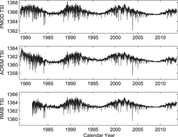
Figure 1. Three composites: PMOD TSI (Fröhlich & Lean 1998; Fröhlich 2006; top panel), ACRIM TSI (Willson 1997; Willson & Mordvinov 2003; Willson 2014; middle panel), and RMIB TSI (Dewitte et al. 2004; Mekaoui & Dewitte 2008; bottom panel).
Download figure:
Standard image High-resolution image2.2. Cross-correlation (CC) Analysis between TSI and Magnetic Field Activity
The Magnetic Plage Strength Index (MPSI) and the Mount Wilson Sunspot Index (MWSI) can reflect the solar full-disk magnetic activity, which comes from the solar full-disk magnetic magnetogram measured at Mount Wilson Observatory (MWO) since the 1970s (Chapman & Boyden 1986; Parker et al. 1998). For each magnetogram at the 150-foot solar tower of MWO, an MPSI value and an MWSI value are calculated. The MPSI values are calculated as follows. First, all pixels, where the absolute values of the magnetic field strength are between 10 and 100 G, are selected in the magnetogram. Then, the absolute values of the magnetic field strengths of these pixels are summed. Finally, the summation is divided by the total number of pixels (regardless of magnetic field strength) in the magnetogram. The MWSI values are also calculated in much the same manner as the MPSI, but summation is only done for pixels where the absolute value of the magnetic field strength is greater than 100 G (Howard et al. 1980, 1983; Ulrich 1991; Ulrich et al. 1991; Li et al. 2014; Xiang et al. 2014). The MPSI and MWSI should represent the activity of weak magnetic field (with plage/facular regions and outside of sunspots) on the solar full disk and the strong magnetic field activity (in sunspots) on the disk, respectively (Chapman & Boyden 1986; Parker et al. 1998; Li et al. 2014; Xiang et al. 2014). The two indices can be downloaded from MWO (http://obs.astro.ucla.edu/intro.html).
In order to study the phase relationship between TSI and MWSI at timescales of solar cycles, we performed a CC analysis of three TSI composites versus MWSI, and the results are shown in Figure 2. In this figure, the abscissa indicates the shift of TSI with respect to MWSI along the calendar-time axis, with negative values representing backward shifts. As this figure (left panel) shows, when PMOD TSI has no shift versus MWSI, the correlation coefficient (cc) is just 0.105 (called cc0). However, when PMOD TSI is shifted backward by 24 days with respect to MWSI along the calendar-time axis, the cc between PMOD TSI and MWSI peaks at 0.461 (called ccpeak), with an obvious increase. In order to test statistical significance of the difference of ccpeak and its corresponding  an independent sample set that contains 8000 randomly selected values from the total 9242 values of MWSI is selected. Then the sample set is utilized to calculate the correlation coefficient with the corresponding PMOD TSI, obtaining a paired set of correlation coefficients, one at TSI 24-day backward shift ccpeak (abscissa) and the other at no shift cc0 (ordinate). Such a procedure is repeated 10,000 times, and the obtained 10,000 points are shown in Figure 3. The diagonal line is shown in the figure as well. When a certain point locates above the diagonal, cc0 is larger than
  and when under the diagonal, ccpeak is larger. All points are under the diagonal, the probability is about 100%, and thus PMOD TSI statistically significantly lags behind MWSI by about 24 days (about a solar rotation cycle) at timescales of solar cycles.
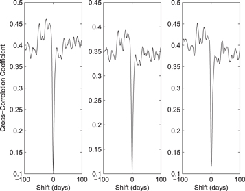
Figure 2. Cross-correlation coefficients of the three TSI composites vs. MWSI. The abscissa indicates the shift of TSI vs. MWSI along the calendar-time axis, with negative values representing backward shifts. Those for MWSI vs. PMOD TSI, ACRIM TSI, and RMIB TSI are shown in the left, middle, and right panels, respectively.
Download figure:
Standard image High-resolution image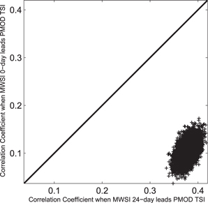
Figure 3. Statistical significance of the difference between correlation coefficients of MWSI with PMOD TSI and those of both when the latter is 24-day backward shifted vs. the former.
Download figure:
Standard image High-resolution imageThe middle panel of Figure 2 shows the result of CC analysis of ACRIM TSI versus MWSI. As it shows, the cc peaks at 0.394 (called ccpeak) when ACRIM TSI is shifted backward by 24 days with respect to MWSI along the calendar-time axis, and the cc value is 0.109 (called cc0) at no shift. Then, we test statistical significance of the difference of ccpeak and its corresponding  First, an independent sample set that contains 8000 randomly selected values from the total 9242 values of MWSI is selected, and then the sample set is utilized to calculate the correlation coefficient with the corresponding ACRIM TSI, obtaining a paired set of correlation coefficients, one at TSI 24-day backward shift ccpeak (abscissa) and the other at no shift cc0 (ordinate). Such a procedure is repeated 10,000 times, and Figure 4 shows the obtained paired cc values. All points are under the diagonal, the probability is about 100% that ccpeak is larger than
  and ACRIM TSI statistically significantly lags behind MWSI by about 24 days (about one solar rotation cycle) at timescales of solar cycles.

Figure 4. Statistical significance of the difference between correlation coefficients of MWSI with ACRIM TSI and those of both when the latter is 24-day backward shifted vs. the former.
Download figure:
Standard image High-resolution imageThe right panel of Figure 2 shows the result of CC analysis of RMIB TSI versus MWSI. The cc value is 0.135 (called cc0) when RMIB TSI has no shift versus MWSI. The cross-correlation coefficient peaks when the relative phase shift between them is −24 and −48 days, and the corresponding peak values are 0.442 and 0.452, respectively. The peak value around the 24-day backward shift is only smaller than that around the 48-day backward shift by 0.01; the difference between them should be negligible. Moreover, the above analysis indicates that PMOD TSI and ACRIM TSI should lag behind MWSI by about one solar rotation cycle. Thus, we select the peak value around the RMIB TSI 24-day backward shift as  Then, we test the statistical significance of the difference of ccpeak and its corresponding
  An independent sample set that contains 7000 randomly selected values from the total 8261 values of MWSI is selected, and then the sample set is utilized to calculate the correlation coefficient with the corresponding RMIB TSI, obtaining a paired set of correlation coefficients, one at TSI 24-day backward shift ccpeak (abscissa) and the other at no shift cc0 (ordinate). Such a procedure is repeated 10,000 times, and Figure 5 shows the obtained paired cc values. All points are under the diagonal, the probability is about 100% that ccpeak is larger than
  and RMIB TSI statistically significantly lags behind MWSI by about 24 days (about one solar rotation cycle) at timescales of solar cycles.

Figure 5. Statistical significance of the difference between correlation coefficients of MWSI with RMIB TSI and those of both when the latter is 24-day backward shifted vs. the former.
Download figure:
Standard image High-resolution imageIf the inter-solar-cycle variation of TSI is really related to MWSI, the TSI should be highly correlated and accurately in phase with MWSI at timescales of solar cycles. The CC analysis indicates that the correlation coefficients of MWSI with PMOD TSI, ACRIM TSI, and RMIB TSI are only 0.105, 0.109, and 0.135, respectively, when TSI is not shifted with respect to MWSI along the calender-time axis, so the three TSI composites should be weakly correlated with MWSI. Furthermore, the above analysis indicates that the three TSI composites should not be in phase with MWSI at timescales of solar cycles. Thus, the inter-solar-cycle variation of TSI should not be related to strong magnetic field activity on the disk, which is represented by MWSI.
By using the same method, the CC analysis is used to analyze the relationship of the three TSI composites with MPSI at timescales of solar cycles, and the results are shown in Figure 6. In this figure, the abscissa indicates the shift of TSI with respect to MPSI along the calendar-time axis, with negative values representing backward shifts.

Figure 6. Cross-correlation coefficients of the three TSI composites vs. MPSI. The abscissa indicates the shift of TSI vs. MPSI along the calendar-time axis, with negative values representing backward shifts. Those for MPSI vs. PMOD TSI, ACRIM TSI, and RMIB TSI are shown in the left, middle, and right panels, respectively.
Download figure:
Standard image High-resolution imageThe left panel of Figure 6 shows the result of CC analysis of PMOD TSI versus MPSI. When PMOD TSI has no shift versus MPSI, the cc value between them is 0.582 (called cc0), and when PMOD TSI is shifted backward by 23 days with respect to MPSI along the calender-time axis, the cc peaks at 0.633 (called ccpeak), only an increase of 0.051. Then, we test the statistical significance of the difference between ccpeak and its corresponding  An independent sample set that contains 8000 randomly selected values from the total 9242 values of MPSI is selected, and then the sample set is utilized to calculate the correlation coefficient with the corresponding PMOD TSI, obtaining a paired set of correlation coefficients, one at TSI 23-day backward shift ccpeak (abscissa) and the other at no shift cc0 (ordinate). Such a procedure is repeated 10,000 times, and Figure 7 shows the obtained paired cc values. There are only 5500 points under the diagonal. Thus, the difference between ccpeak and its corresponding cc0 is statistically insignificant, and PMOD TSI should be in phase with MPSI at timescales of solar cycles.
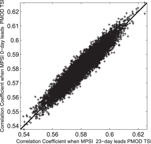
Figure 7. Statistical significance of the difference between correlation coefficients of MPSI with PMOD TSI and those of both when the latter is 23-day backward shifted vs. the former.
Download figure:
Standard image High-resolution imageThe middle panel of Figure 6 shows the result of CC analysis of ACRIM TSI versus MPSI. The cc value is 0.544 at no shift (called cc0), and the cc peaks at 0.589 (called ccpeak) when ACRIM TSI is shifted backward by 21 days with respect to MPSI along the calendar-time axis. Though the cross-correlation coefficient peaks around about ACRIM TSI 21-day backward shifts, the ccpeak is only lager than cc0 by 0.045. Then, we test the statistical significance of the difference between ccpeak and its corresponding  An independent sample set that contains 8000 randomly selected values from the total 9242 values of MPSI is selected, and then the sample set is utilized to calculate the correlation coefficient with the corresponding ACRIM TSI, obtaining a paired set of correlation coefficients, one at TSI 21-day backward shift ccpeak (abscissa) and the other at no shift cc0 (ordinate). Such a procedure is repeated 10,000 times, and Figure 8 shows the obtained paired cc values. There are only 6850 points under the diagonal. Thus, the difference between ccpeak and its corresponding cc0 is statistically insignificant, and ACRIM TSI should be in phase with MPSI at timescales of solar cycles as well.
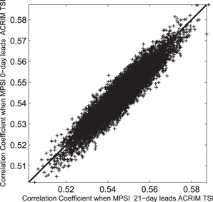
Figure 8. Statistical significance of the difference between correlation coefficients of MPSI with ACRIM TSI and those of both when the latter is 21-day backward shifted vs. the former.
Download figure:
Standard image High-resolution imageThe right panel of Figure 6 shows the result of CC analysis of RMIB versus MPSI. The cc peaks at 0.615 (called ccpeak) when RMIB TSI is shifted backward by 24 days with respect to MPSI along the calendar-time axis, and the cc value is 0.569 (called cc0) at no shift. We can see that the ccpeak is only larger than cc0 by 0.046. Then, we test statistical significance of the difference of ccpeak and its corresponding  An independent sample set that contains 7000 randomly selected values from the total 8261 values of MPSI is selected, and then the sample set is utilized to the calculate correlation coefficient with the corresponding RMIB TSI, obtaining a paired set of correlation coefficients, one at TSI 24-day backward shift ccpeak (abscissa) and the other at no shift cc0 (ordinate). Such a procedure is repeated 10,000 times, and Figure 9 shows the obtained paired cc values. There are only 5438 points under the diagonal. Thus, the difference between ccpeak and its corresponding cc0 is statistically insignificant, and RMIB TSI should be in phase with MPSI at timescales of solar cycles as well.
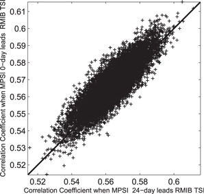
Figure 9. Statistical significance of the difference between correlation coefficients of MPSI with RMIB TSI and those of both when the latter is 24-day backward shifted vs. the former.
Download figure:
Standard image High-resolution imageOn the other hand, the CC analysis shows that the correlation coefficients of TSI with MPSI should be obviously higher than those of TSI with MWSI, so we also test the statistical significance of the difference between these correlation coefficients. The correlation coefficients of MPSI with PMOD TSI, ACRIM TSI, and RMIB TSI are 0.582, 0.544, and 0.569, respectively, while the correlation coefficients of MWSI with PMOD TSI, ACRIM TSI, and RMIB TSI are only 0.105, 0.109, and 0.135, respectively. Following the method used in Li et al. (2002), the probability is about 99% that the correlation coefficient of TSI with MPSI is larger than that of TSI with MWSI.
The CC analysis of three TSI composites versus MPSI indicates that three TSI composites should be accurately in phase with MPSI, and the correlation coefficients of MPSI versus PMOD TSI, ACRIM TSI, and RMIB TSI are about 0.582, 0.544, and 0.569, respectively, so three TSI composites should be moderately correlated with MPSI at timescales of solar cycles. Furthermore, the statistical significance test shows that the correlation coefficients of three TSI with MPSI are statistically significantly larger than those of three TSI composites with MWSI. Consequently, the inter-solar-cycle variation of TSI should be more related to weak magnetic field activity on the disk, which is represented by MPSI. Thus, in the next section we further validate the relation of three TSI composites with MPSI and MWSI at timescales of solar cycles.
2.3. The Cross Wavelet Transform (XWT) and Wavelet Coherence (WTC) Analysis of TSI and MPSI
The XWT and WTC are widely used to analyze the nonlinear behavior and expose common power and relative phase in time-frequency space between the two time series (Grinsted et al. 2004; Li 2008; Li et al. 2009; Deng et al. 2012; Kong et al. 2014). The XWT of the two time series Xn and Yn is defined as  where WX and WY are the continuous wavelet transforms and the asterisk denotes complex conjugation. Furthermore, the cross wavelet power is defined as
  and the complex argument
  can be interpreted as the local relative phase between Xn and Yn in time-frequency space (Grinsted et al. 2004; Li et al. 2009; Deng et al. 2013). Cross wavelet power reveals areas with high common power. The WTC is another useful method, which can measure how coherent the XWT is in time-frequency space and find significant coherence even though the common power is low. The WTC can be thought of as the local correlation between two time series in time-frequency space, and it is a powerful method for testing proposed linkages between two time series (for details, see Grinsted et al. 2004). Furthermore, since the cross wavelet spectrum is unsuitable for significance testing the interrelation between two processes (Maraun & Kurths 2004; Li et al. 2009), WTC is necessary. The WTC of two time series X and Y is defined as (Grinsted et al. 2004; Li et al. 2009)
where S is a smoothing operator. This definition closely resembles a traditional correlation coefficient, so it can be thought of as a localized correlation coefficient in time-frequency space. The smoothing operator S can be written as

where Sscale denotes smoothing along the wavelet scale axis and Stime denotes smoothing in time. For the Morlet wavelet a suitable smoothing operator is given as (Grinsted et al. 2004; Li et al. 2009)


where c1 and c2 are normalization constants and  is the rectangle function. The value of the factor is 0.6, which is the empirically determined scale decorrelation length for the morlet wavelet (Torrence & Compo 1998; Grinsted et al. 2004; Li et al. 2009). In practice both convolutions are done discretely, and therefore the normalization coefficients are determined numerically. Additionally, the statistical significance level of the WTC is estimated by Monte Carlo methods (Grinsted et al. 2004; Li et al. 2009). In this study, we employ the codes provided by Grinsted et al. (2004) to show the XWT and WTC of the TSI and MPSI in order to investigate their relationship.
The whole measured MPSI spans 12,699 days, but some days do not have observations because of the terrible weather. The MPSI has observation records in 9242 of the 12,699 days from 1978 November 17 to 2013 August 23, and it is an uneven time series. In order to use XWT and WTC to analyze the relation of TSI to MPSI at timescales of a solar cycle, we calculate the monthly mean MPSI as follows. The values of the availably daily MPSI are summed over a month, and then the summation is divided by the number of available data in a month. The monthly mean PMOD TSIs are also calculated in much the same manner as that of the MPSI. The XWT and WTC spectra of monthly mean PMOD TSI and MPSI are shown in Figure 10. The XWT and WTC show that the two series are in phase and have significant common power at timescales of a solar cycle, because almost all arrows point right in this area. We also further calculate the mean phase angle at a certain period scale, which indicates the mean value of all phase angles at a certain period scale from the beginning to the end of the time interval considered, and the result is shown in Figure 11. The corresponding standard deviations of the mean phase angles are also obtained and are given in Figure 11 as well. As it shows, the mean phase angles of PMOD TSI and MPSI and the corresponding standard deviations are very puny on timescales of 9–11 yr (about a solar cycle); the two series should be in phase at this timescale. In all, Figures 10 and 11 indicate that the PMOD TSI is highly correlated and in phase with MPSI at timescales of a solar cycle, and the inter-solar-cycle variation of TSI is related to MPSI at these timescales. We also use XWT and WTC to analyze the relationship of ACRIM TSI and RMIB TSI with MPSI, and the two TSI composites give almost the same results. In this paper we do not show the figures.
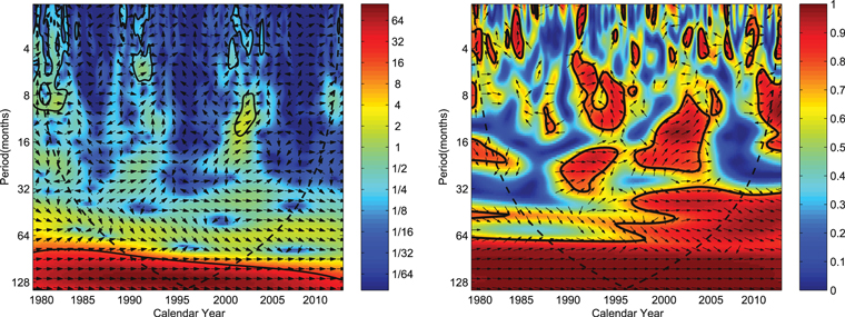
Figure 10. Cross wavelet transform (left) and wavelet coherence (right) of the monthly mean PMOD TSI and MPSI. The 95% confidence level is shown as a thick contour, and the black dashed line indicates the cone of influence where edge effects might distort the picture. The relative phase relation is shown as arrows (with in-phase pointing right, anti-phase pointing left, and PMOD TSI leading MPSI by 90° pointing straight down).
Download figure:
Standard image High-resolution image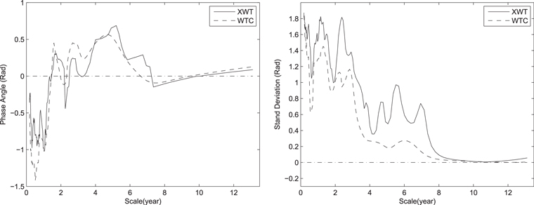
Figure 11. Phase angles of the PMOD TSI and MPSI as a function of periods (left) and their corresponding standard deviations (right) with the XWT (solid lines) and WTC (dashed lines) methods used.
Download figure:
Standard image High-resolution image2.4. The WTC and Partial Wavelet Coherence (PWC) Analysis of TSI and MWSI
The CC analysis of TSI with MWSI indicates that TSI lags behind MWSI by about a solar rotation cycle, and we should use XWT and WTC to validate the phase relationship of the two time series. However, the phase angle of TSI and MWSI is small at timescales of a solar cycle. If we use the XWT and WTC to validate the phase angle of the two time series, the value of the phase angle of the two time series almost equals the corresponding standard deviations and should be uncertain and insignificant. Furthermore, when we investigate the relation of TSI with MWSI, the effect of MPSI should be eliminated. Consequently, we do not analyze the phase relationship of TSI with MWSI, while another method is used to validate the relation of them.
In probability theory and statistics, partial correlation measures the degree of association between two random variables, with the effect of a set of controlling random variables removed. PWC is a technique similar to partial correlation that is utilized to find the results of WTC between two time series y and x1 after eliminating the effect of the time series x2 (Ng & Chan 2012). The PWC squared (after eliminating the effect of the time series x2) can be defined by an equation that is similar to the partial correlation squared, as (Mihanović et al. 2009; Ng & Chan 2012)
which is similar to the simple WTC, ranging from 0 to 1. In this case, a high WTC squared shown at where a low PWC squared was found implies that the time series x1 does not have a significant effect on the time series y at that particular time-frequency space. In this study, the WTC (codes provided by Grinsted et al. 2004) is used investigate the relation of TSI and MWSI, and PWC (codes provided by Ng & Chan 2012) is used to find the results of WTC between PMOD TSI and MWSI after eliminating the effect of MPSI.
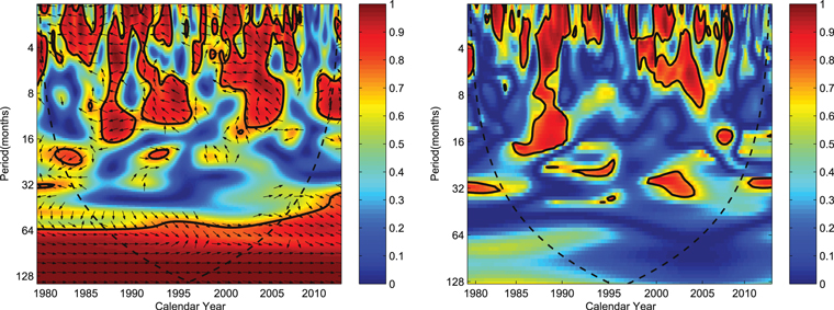
The monthly mean MWSI is also calculated, and the WTC and PWC spectra of monthly mean PMOD TSI and MWSI are shown in Figure 12. As it shows, though the WTCs of the two time series have common significant power at timescales of a solar cycle, the arrows point down a little at this timescale, the PWC shows very low power, and the two time series have no common significant region of above 95% confidence level at this timescale. Combining WTC and PWC, we can conclude that the variation of TSI at a solar cycle is not related to solar strong magnetic activity on the disk, which is represented by MWSI. At the same time, both WTC and PWC show that the two time series have common significant regions of above 95% confidence level at short timescales, it is inferred that the variation of TSI at short timescales is highly related to solar strong magnetic activity, which is represented by MWSI. This result is the same as in earlier papers (Willson et al. 1981; Solanki et al. 2003; Domingo et al. 2009; Withbroe 2009; Li et al. 2012). We also use WTC and PWC to analyze the relationship of ACRIM TSI and RMIB TSI with MWSI, and the relation of them gives almost the same results. In this paper we do not show the figures.
Figure 12. Wavelet coherence (left) and partial wavelet coherence (right) of the monthly mean PMOD TSI and MWSI. The 95% confidence level is shown as a thick contour, and the black dashed line indicates the cone of influence where edge effects might distort the picture.
Download figure:
Standard image High-resolution image
3. CONCLUSION AND DISCUSSION
One of the theories of TSI variation indicates that the solar convective envelope likes a "thermal superconductor" with a huge thermal inertia, and the same thermal inertia makes possible the irradiance fluctuations due to "superficial" photospheric magnetic structures (Spruit 1991; Solanki et al. 2013). At the same time, in models of reconstructing TSI, the SATIR model assumes that the irradiance variation should be entirely caused by the evolution of the solar surface magnetic field on timescales of half a day to one Schwabe solar cycle (Fligge et al. 2000; Krivova et al. 2003, 2011; Solanki et al. 2005, 2013; Unruh et al. 2008). Thus, we analyze the relation of TSI with solar magnetic field activity and attempt to investigate what causes the inter-solar-cycle variation of TSI.
CC analysis of MWSI with three TSI composites shows that the correlation coefficients of MWSI with PMOD TSI, ACRIM TSI, and RMIB TSI are only 0.1050, 0.1085, and 0.1352, respectively, and the three TSI composites lag behind MWSI by about one solar rotation cycle, so the TSI should be weakly correlated with MWSI and not be in phase with MWSI at timescales of solar cycles. Furthermore, the WTC and PWC indicate that the inter-solar-cycle variation of TSI is not related to solar strong magnetic activity as well, which is represented by MWSI.
CC analysis of MPSI with three TSI composites shows that three TSI are accurately in phase with MPSI at timescales of solar cycles, and the correlation coefficients of MWSI with PMOD TSI, ACRIM TSI, and RMIB TSI are about 0.582, 0.544, and 0.569, respectively. The three TSI composites are moderately correlated with MPSI at timescales of solar cycles. The statistical significance test indicates that the correlation coefficient of three TSI composites with MPSI is statistically significantly higher than that of three TSI composites with MWSI. So it looks like the inter-solar-cycle variation of TSI should be related to the solar weak magnetic field activity on the full disk, which is represented by MPSI. Moreover, the XWT and WTC show that TSI is highly related to and actually in phase with MPSI as well, and the variation of TSI is related to MPSI at timescales of a solar cycle. On the other hand, TSI lags behind MWSI by about one solar rotation cycle, and TSI is actually in phase with MPSI. That is to say, MPSI should lag behind MWSI by about one solar rotation cycle. The reason is that the relatively early MWSI should be one source of the relatively late MPSI (Xiang et al. 2014). Consequently, the phase relationship among TSI, MPSI, and MWSI in our study should coincide with Xiang et al. (2014), and it should indirectly validate that the MPSI components partly come from relatively early MWSI measurements. Spruit (1991) indicated that the solar convective envelope likes a "thermal superconductor" with a huge thermal inertia, and the same thermal inertia makes possible the irradiance fluctuations due to "superficial" photospheric magnetic structures. Our finding provides evidence that the inter-solar-cycle variation of TSI is due to the "superficial" photospheric weak magnetic structures and is also one of the reasons why additional irradiance variations with origins deeper in the Sun have not been observed so far.
We thank the anonymous referee for their careful reading of the manuscript and constructive comments which improved the original version. The authors thank PMOD science team and ACRIM science team for making the two TSI composites and Steven Dewitte for providing the RMIB TSI composite. This study includes data (MPSI and MWSI) from the synoptic program at the 150-foot solar tower of the Mount Wilson Observatory. The Mount Wilson 150-foot solar tower is operated by UCLA, with funding from NASA, ONR, and NSF, under agreement with the Mount Wilson Institute. The authors are especially indebted to Ke-Jun Li for his constructive ideas and helpful suggestions on the manuscript. This work is supported by the National Natural Science Foundation of China (11273057 and 11221063), the 973 programs 2012CB957801 and 2011CB811406, and the Chinese Academy of Sciences.