


ABSTRACT
Laboratory studies predict that the photo-dissociation of H2O by solar  photons in the comae of comets should lead to a small percentage of OH in high rotational states of the
  electronic state. These states should promptly emit a near-ultraviolet (near-UV) photon in a transition to the
  state. From there, the radicals decay to the lowest rotational states by direct rotational transitions and via ro-vibrational cascade in the 1-0 vibrational band, all within the
  state. Normally in Earth-based observations the lines are extremely weak compared to the fluorescence of OH in sunlight. Since the prompt emission rate is directly proportional to the column density of water, whereas the fluorescent emission of OH is proportional to the column density of OH, the lines due to prompt emission are relatively strongest very close to the nucleus, a region not often accessible from Earth. We report here the first spectrally resolved detection of near-UV prompt emission by cometary OH, as seen in the bright comet Hyakutake (C/1996 B2), on the day of its closest approach to Earth. All the expected doublets are seen, in both the P and Q branches, up to rotational quantum number N' = 22 with relative strengths in good agreement with the laboratory results. The fluxes of the lines are in agreement with what one expects from the various measurements of the water production rate of the comet, including that deduced from the OH fluorescent lines in these spectra.
Export citation and abstract BibTeX RIS
1. INTRODUCTION
Among volatiles present in the comae of comets, the molecule H2O is the dominant species in nearly all comets at heliocentric distances less than roughly 2.5–3 AU. This high abundance of water has been known for more than half a century, first from ground-based observations of the OH radical in the near-ultraviolet (near-UV) and later from space-based observations of  further in the ultraviolet (see, e.g., the review by Delsemme 1973), but direct detection of H2O was first achieved by Mumma et al. (1986), who used the Kuiper Airborne Observatory to observe the
  band of H2O near 2.7 μm from comet 1 P/Halley.
The (0-0) band of the  transition of OH, centered at about 3085 Å, is often the strongest feature in a cometary spectrum. This 0-0 band has been extensively observed and interpreted. It has been shown, for example, that the emission in this band by most comets is almost entirely due to fluorescence (e.g., Schleicher & A'Hearn 1988) and the spatial distribution has been successfully modeled, with what is now the widely used vectorial model (e.g., Festou 1981, and references therein), as due primarily to photodissociation of H2O. The direct signature of H2O dissociating into OH comes from the fact that the dissociation process, a very large part of which is due to solar
  radiation, produces OH in highly rotationally excited states within the
  electronic state, a process that was first studied in detail by Carrington (1964), although numerous other studies exist, a few prior to Carringtons work and many thereafter. Bertaux (1986) was the first, as far as we are aware, to point out that the signature of this process should be observable in comets. Bertaux deduced an effective g-factor (prompt OH photons per second per molecule of H2O) for the sum of all the A–X prompt transitions of
  based on earlier discussions of the various dissociation branches by Festou (1981). The first reported measurements were by Budzien & Feldman (1991), who used the spatial and spectral variation in the low-resolution spectra from IUE of comet IRAS–Araki–Alcock (1983 VII = 1983 H1). They deduced a g-factor of
  for the solar conditions at the time of comet IRAS–Araki–Alcock, a time of moderately high solar activity. Most recently, Combi et al. (2005, pp. 523–552) have summarized all the destruction mechanisms of H2O. They find a range of rates into the
  state varying with solar activity over
  , a range encompassing the earlier estimates by Bertaux and by Budzien and Feldman. This should be compared to a total photodestruction rate of H2O that varies over
  with solar activity. Prompt emission by OH in the near-infrared, first pointed out by Mumma et al. (2001), has also been studied by Bonev et al. (2004), Bonev et al. (2006) and Bonev & Mumma (2006). These are purely ro-vibrational transitions within the
  state, involving levels
  . These levels can be populated both directly in the dissociation process and by cascades from higher rotational states that are populated both from the
  state and from the direct dissociation.
We present here the details of high-resolution observations of prompt emission in numerous individual lines of the  transition of OH from comet Hyakutake (1996 B2) at a time of low solar activity. These prompt emissions can be important for studying the spatial distribution of the H2O released from the nucleus, just as can the direct observations of H2O in the infrared and submillimeter. The bulk spatial distribution of H2O in comets is, of course, very different from the bulk distribution of OH and the combination of the two can test the hydrodynamics of the gas in the coma. Here we present the details of the observations, the identifications of the numerous lines, and the relationship of the emission rate to the production of H2O.
2. OBSERVATIONS
Comet Hyakutake (C/1996 B2) was observed with the 4 m Mayall Telescope at Kitt Peak National Observatory using the echelle spectrograph during a half-night on 1996 March 26. The observational circumstances are given in Table 1, which is adapted from Meier et al. (1998), who also provide more extensive details. Analyses of other results from the spectra were presented by Meier et al. (1998), by Kim et al. (2003), and by A'Hearn et al. (2014). Meier et al. also discuss the reduction of the data. Individual exposures are given in Table 2, with the original data-file ID, the mid-time of each exposure, and the offset from the photocenter. The exposures were combined, weighted by exposure time and corrected for atmospheric extinction, to produce single spectra nominally on the nucleus and with offsets of 2, 7, and 10 arcsec sunward. The slit was oriented E–W for most spectra and since the comet was passing over the celestial pole during the observing window, the offsets were very approximately perpendicular to the length of the slit, which had dimensions 0.87 × 7.84 arcsec or 68 × 580 km projected at the comet. Since guiding was done at visible wavelengths and the atmospheric refraction is much larger at these ultraviolet wavelengths, the actual offsets are typically 100 km larger at the near-UV wavelengths of interest and vary by 10 s of km over the spectral range of interest. This, coupled with the fact that the photocenter was obviously fuzzy, means that the offsets are not precise. While guiding the long exposure for the 7 arcsec offset, there appeared visually to be a fragment tailward of the nucleus that was sketched in the observing log, so there may have been additional localized transient activity during that particular exposure. Tailward moving fragments were a widely observed feature in this comet over a 10 day to 2 week period nearly centered on our observations (e.g., Desvoivres et al. 2000; Capria et al. 2002), lending credence to the visual observation of a small fragment.
Table 1. Observational Geometry
| UTC | r |

|
Δ | dΔ/dt | Phase | Scale | Slit Size |
|---|---|---|---|---|---|---|---|
| 1996 Mar | (AU) | (km s−1) | (AU) | (km s−1) | (degree) | (km arcsec−1) | (km) |
| 26.3–26.5 | 1.02 | −36.7 | 0.11 | +18.3–20.8 | 75–77 | 78 | 68 × 580 |
Download table as: ASCIITypeset image
Table 2. Individual Exposures
| Exp ID | Mid-UTC | Exp Time | AirMass | Offset |
|---|---|---|---|---|
| (s) | (arcsec) | |||
| coo23 | 6:02:57 | 600 | 1.530 | 0 |
| coo24 | 6:16:02 | 600 | 1.513 | 0 |
| coo35 | 7:04:45 | 600 | 1.468 | 7 |
| coo36 | 7:17:27 | 600 | 1.460 | 7 |
| coo37 | 7:31:14 | 600 | 1.453 | 10 |
| coo38 | 7:44:05 | 600 | 1.449 | 10 |
| coo39 | 8:31:03 | 600 | 1.443 | 10 |
| coo40 | 8:54:26 | 1800 | 1.445 | 10 |
| coo41 | 9:27:58 | 1800 | 1.458 | 10 |
| coo42 | 10:15:54 | 3600 | 1.489 | 2 |
| coo43 | 11:04:23 | 1800 | 1.544 | 0 |
Download table as: ASCIITypeset image
The instrument line shape can be reasonably approximated as a triangle with FWHM = 0.18 Å, although see the discussion of extraction of fluxes below, and the spectral range, covering 42 orders of the echelle, was roughly 3000–4500 Å. The spectral range of primary interest here is 3140–3250 Å. The wavelength scale was set initially by using thorium–argon lamp spectra. However, the paucity of Th–Ar lines in this spectral region led us to further adjust the wavelength scale using the fluorescent lines of OH in this region. As we will see below, there are some systematic offsets from calculated line positions by 0.1–0.2 Å. The complete spectra, including the portions discussed here, are available at NASA's Planetary Data System (A'Hearn et al. 2015).
3. ANALYSIS
Figures 1 and 2 and Tables 3 and 4 identify the lines that have been associated with prompt emission in the P and Q branches of the 0-0 band of OH ( –
– ). The four spectra in each figure correspond to the four spatial positions, offset vertically for clarity. The features due to prompt emission are identified by short, vertical lines near the top and bottom of the figures. In Figure 2 there are also numerous, much stronger lines that correspond to well known, fluorescent transitions of the 1-1 band and which involve very low-lying rotational levels. The prompt lines of the R branch are badly contaminated by the low-lying fluorescent lines of the 0-0 band and are not analyzed here.
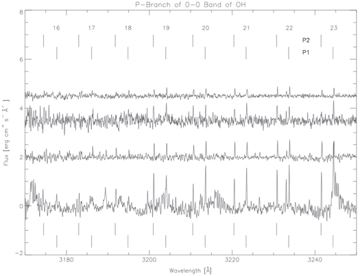
Figure 1. Spectrum of prompt emission by OH in the P branch of the 0-0 band of the A  –X
–X  transition. Wavelengths are in air. From bottom to top are the spectra on the photocenter and at offsets of 2, 7, and 10 arcsec (nominal), plotted with vertical displacements for clarity. Vertical ticks across the top of the figure indicate the features identified as due to prompt emission, labeled with the lower rotational quantum number, N''. As expected, the P branch extends to N one greater than in the Q branch, since these have a common upper state.
Download figure:
Standard image High-resolution image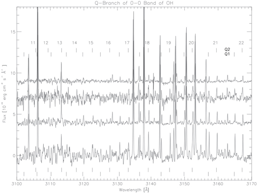
Figure 2. Spectrum of prompt emission by OH in the Q branch of the 0-0 band of the A  –X
–X  transition. Wavelengths are in air. From bottom to top are the spectra on the photocenter and at offsets of 2, 7, and 10 arcsec (nominal), plotted with vertical displacements for clarity. The strongest lines, some of which are off scale, are due to fluorescence in the 1-1 band at low rotational quantum numbers. Vertical ticks across the top of the figure indicate the features identified as due to prompt emission, labeled with the lower rotational quantum number, N''.
Download figure:
Standard image High-resolution imageTable 3. Prompt Emission Lines: P Branch
| J' | N' | Air λ | Air λ | Flux | |||
|---|---|---|---|---|---|---|---|
| Calculated | Measured | 0'' | 2'' | 7'' | 10'' | ||
| (Å) | (Å) | ( ) ) |
|||||
| 22.5 | 23 | 3244.35 | 3244.47 | 42 | 10 | 13 | 5.0 |
| 23.5 | 23 | 3241.45 | 3241.56 | 25 | 10 | 7.0 | 4.0 |
| 21.5 | 22 | 3233.65 | 3233.77 | 20 | 10 | 7.2 | 5.2 |
| 22.5 | 22 | 3230.73 | 3230.85 | 22 | 9.9 | 14 | 4.2 |
| 20.5 | 21 | 3223.37 | 3223.49 | 26 | 9.9 | 11 | 5.4 |
| 21.5 | 21 | 3220.42 | 3220.53 | 22 | 11 | 12 | 5.0 |
| 19.5 | 20 | 3213.48 | 3213.59 | 24 | 10 | 7.6 | 6.7 |
| 20.5 | 20 | 3210.6 | 3210.6 | 14 | 7.2 | 9.3 | 5.7 |
| 18.5 | 19 | 3203.98 | 3204.1 | 30* | 8.5 | 7.8 | 4.4 |
| 19.5 | 19 | 3200.96 | 3201.08 | 24 | 11 | 16 | 4.7 |
| 17.5 | 18 | 3194.85 | 3195.0 | 6* | 3.4 | 7* | 3.5 |
| 18.5 | 18 | 3191.78 | 3191.96 | 14 | 5.8 | 3.3 | 2.7 |
| 16.5 | 17 | 3186.08 | 3186.2 | 10* | 4.0 | 1.4* | 3.0 |
| 17.5 | 17 | 3182.97 | 3183.07 | 15 | 6.4 | 2.1 | 3.5 |
| 15.5 | 16 | 3177.68 | 3177.64 | 9.2 | 1.1 | 3.3 | 2.1 |
| 16.5 | 16 | 3174.48 | 3174.35 | 9.2 | 4.3 | 8.0 | 2.8 |
| Total | 313 | 130 | 129 | 67 | |||
Download table as: ASCIITypeset image
Table 4. Prompt Emission Lines: Q Branch
| J' | N' | Air Wavelength | Air Wavelength | Flux | |||
|---|---|---|---|---|---|---|---|
| Calculated | Comet Measured | 0'' | 2'' | 7'' | 10'' | ||
| (Å) | (Å) | ( ) ) |
|||||
| 21.5 | 22 | 3167.16 | 3167.39 | 49 | 22 | 35 | 8.8 |
| 22.5 | 22 | 3164.81 | 3165.05 | 33 | 12 | 13 | 6.3 |
| 20.5 | 21 | 3159.50 | 3159.73 | 51 | 25 | 20 | 11.9 |
| 21.5 | 21 | 3157.11 | 3157.35 | 50 | 22 | 22 | 9.0 |
| 19.5 | 20 | 3152.29 | 3152.5 | 56* | 22 | 42 | 13.1 |
| 20.5 | 20 | 3149.84 | 3150.07 | 66 | 26 | 22 | 16.0 |
| 18.5 | 19 | 3145.51 | 3145.75 | 42 | 21 | 19 | 8.3 |
| 19.5 | 19 | 3143.01 | 3143.09 | 52 | 18 | 29 | 8.0 |
| 17.5 | 18 | 3139.15 | 3139.26 | 49 | 22 | 29 | 10.7 |
| 18.5 | 18 | 3136.59 | 3136.71 | 29 | 17* | 66 | 7.6* |
| 16.5 | 17 | 3133.22 | 3133.3 | 22* | 18 | 13* | 14.5 |
| 17.5 | 17 | 3130.56 | 3130.70 | 21 | 11 | 9* | 5.8 |
| 15.5 | 16 | 3127.68 | 3127.78 | 42 | 13 | 15 | 5.0 |
| 16.5 | 16 | 3124.93 | 3125.1 | 11* | 17 | 5 | 7.6 |
| 14.5 | 15 | 3122.43 | 3122.6 | 17* | 18 | 8 | 2.5* |
| 15.5 | 15 | 3119.67 | 3119.75 | 35 | 22 | 12* | 9.8 |
| 13.5 | 14 | 3117.76 | 3117.74 | 13 | 22 | 15 | 4.3 |
| 14.5 | 14 | 3114.77 | 3114.98 | 16 | 4* | 7* | 1.8 |
| 12.5 | 13 | 3113.36 | 3113.6 | 17* | 8* | 6* | 0.4* |
| Total | 672 | 338 | 386 | 152 | |||
Download table as: ASCIITypeset image
The tables provide the line identification (via N'' and J'', the quantum numbers of the lower state of the transition) and the calculated wavelength using the term values of Moore & Richards (1971); these calculated wavelengths are in reasonably good agreement with the measured values of Dieke & Crosswhite (1962). Also included are the cometary wavelength as measured in the spectrum at the photocenter, and the measured flux of the line in each of the four spectra. No corrections have been made to the observed wavelengths for Doppler shifts or for possible errors in the original calibration of the wavelength scale.
The intensity of each line was determined first with a routine that fit a Gaussian of fixed halfwidth (consistent with the half width of the triangular slit function) in order to remove residual continuum on either side of the line. In a few cases, typically for what appear to be blends with unidentified lines, the procedure failed to converge. In a very few other cases, the procedure zeroed in on a nearby stronger line. In both of these cases, the residuals between the fitted wavelength and the nominal wavelengths in the observed spectrum were used as a guide, since the offsets (caused by the dearth of wavelength calibration lines in this spectral region) should be smooth with wavelength. In those cases, the strength of the line was estimated by summing the three pixels in the triangular profile if the line seemed to be centered on a pixel or summing the two strongest pixels and half the two adjacent bins if the line seemed to be centered between pixels. These manually estimated strengths are indicated by * in the tables.
Since branching ratios from a common upper level are determined solely by Hönl–London (H–L) factors, which are known for OH, and since the coma is optically thin to emission by high rotational levels in the OH A–X system, the population in any upper level can be determined from measurement of a line in either the P or the Q branch, using the H–L factors to determine the branching ratio. Thus one does not require measurement of all branches to determine the total prompt emission. In general, for these high rotational states, the strengths of P(N''+1) and R(N''–1) lines should be roughly half the strength of the Q(N'') line and this is confirmed by comparing the totals of P and Q at the bottom of Tables 3 and 4. As also can be seen, fluxes decrease substantially from the spectrum that was nominally nucleus-centered to the spectrum offset by 10''. In the following section, we describe a very preliminary and simple model for calculating the relative strength of the features and for determining from the observations the column density of H2O. We also show that the effects of absorption of solar  are significant very close to the nucleus.
4. EMISSION MECHANISM
The photo-dissociation of H2O into OH ( ) was studied experimentally in some detail by Carrington (1964), who measured the prompt emission by OH (
 ). His work has been redone with an indirect technique and in the larger context of other branches, together with more theoretical modeling of the dissociation process, by Harich et al. (2000). Carrington showed that dissociation by
  (1216 Å) led to populations in the v = 0, 1, and 2 levels of
  with relative proportions 1:0.3:
  (Harich et al. subsequently showed that there was also a very small population in v = 3), whereas dissociation by O i at 1304 Å led to populations in those same levels with relative proportions 1.0:0.1:0.00, these latter photons not having enough energy to excite v = 2. Carrington also determined (his Figure 3) the relative populations of the rotational states after dissociation by
  , which differ for v = 0 and v = 1. In the v = 0 state, levels with rotational quantum numbers
  N'
N'  are highly populated with a small population in level N'= 23 and populations in levels N'
  gradually decreasing toward lower rotational energies. The levels populated in v = 1 are primarily 12 through 17, much lower than those in v = 0. Harich et al. deduced a somewhat narrower distribution that differed in details. In Figure 3 we show the relative populations in each rotational level of the v' = 0 state of A
  as estimated by eye in Carrington's Figure 3 and Harich et al.'s Figure 9, upper left panel. We have averaged multiple measurements for the same upper level by Carrington, which show internal scatter up to ±0.1 in these arbitrary units. We have also plotted the normalized intensities of the Q-branch lines in our 0-offset spectrum (summing Q1 and Q2). Note that the Hyakutake intensity at N' = 23 is an estimated upper limit for the undetected line. All three sources show a narrow peak containing levels 17 to 23, with a sharp cutoff above 23 and half power of the low-N side between 16 and 17, and with populations tapering down to a very low level below N' = 12. Since these normalized intensities have an uncertainty of order 0.1 on the arbitrarily normalized scale, the agreement shows clearly that the observed, relative intensities are consistent with prompt emission after photodissociation by
  . This agreement does not rule out alternative processes, but it is at least strongly suggestive that photodissociation dominates.
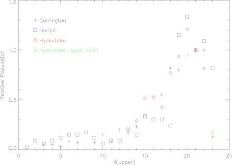
Figure 3. Observed distribution of Q-branch intensities. The observed Q-branch intensities (Q1 + Q2) are compared with the populations of the upper levels produced by photodissociation of H2O by Lyα as measured by Carrington (1964; his Figure 3) and by Harich et al. (2000; their Figure 9 upper left). Each data set has been arbitrarily normalized to illustrate only relative abundance of the given upper state. The differences between the observed intensities and either of the photodissociation measurements are similar to the differences between the two photodissociation measurements.
Download figure:
Standard image High-resolution imageNoting the recently discovered importance of electron impact dissociation near the nucleus of comet 67 P/Churyumov–Gerasimenko at large heliocentric distance (Feldman et al. 2015), we briefly consider electron impact to explain the spectra of Hyakutake (a much more active comet much nearer the Sun). Makarov et al. (2004) have measured the population distribution in the  upper state as produced by electron-impact dissociation using electrons at 100 eV, This spectrum is remarkably different from those in Figure 3, with the highest populations in the lowest rotational levels and extending to levels somewhat higher than N' = 23. Their observed spectrum (their Figure 8) is entirely inconsistent with our observations of Hyakutake. The referee has pointed out that the effects at other electron energies, particularly near the dissociation threshold, may be very different. Möhlmann et al. (1976) have published spectra comparing higher energy electron impact with electron impact near the threshold. In their Figure 1, it is not possible to determine the complete low-energy spectrum, particularly where it is lower in intensity than the high-energy spectrum. Nevertheless, it is clear that both the high-energy and the low-energy spectra show relatively strong lines that are not present in our observed spectrum in the region λλ 3170–3200 Å and very strong lines in the region λλ 3110–3130 Å, where our spectrum shows only weak lines. Furthermore, Möhlmann et al., in their Figure 2, compared the variation of N' = 2 and N' = 27 as a function of electron impact energy and find that the ratio varies roughly between 1/2 and 2—these lines are, respectively, not present and very weak in photodissociation and in our observed spectrum of Hyakutake. Möhlmann et al. further state that at lower energies the wavelengths corresponding to low rotational quantum numbers are relatively stronger than at high impact energies, thus implying that the low energy spectrum will be even less like our observed spectrum than is the 100 eV spectrum of Makarov et al. (2004). Thus it seems clear that electron impact dissociation can only be a minor contributor, even in our near-nucleus (nominally on-nucleus but really at 78 km) exposure. Thus photodissociation of water, primarily by solar
  , is the predominant mechanism causing our observations.
As a cross-check on the emission mechanism, we consider the absolute flux of the emission and ask whether that is consistent with other observations of the release of water by the comet. Meier et al. (1998) had previously estimated a water release rate of  s−1 from the fluorescent lines of OH in these same spectra, but OH averages the water release over time scales of a day or so due to dissociation lifetimes. We are not aware of any near-nucleus observations of water or its prompt products on the same day as our observations, but Bockelée-Morvan et al. (1998) summarized the various published rates of water release available at that time from a variety of observers and concluded that
  s−1 was a reasonable estimate for the time of our observations, but that the uncertainty is about a factor two. (Subsequent updates to some of those values, such as that by Dello Russo et al. 2002, do not alter our assumption.) We started with
  s−1 and then adjusted our calculation to normalize the results to the outermost observation (10 arcsec offset), which is the least sensitive to expected physical processes not included in our oversimplified model but which also has the weakest signal. We assume spherically symmetric radial outflow at 0.75 km s−1, as did Bockelée-Morvan et al. and we initially ignore optical depth effects. Since 1996 was very close to solar minimum, we assume that the dissociation rate into
  is that given by Combi et al. (2005, pp. 523–552) for solar minimum,
  s−1 at r = 1 AU (the correction to 1.02 AU is negligible to the accuracy needed). Carrington (1964) found that 77% of these go to the v' = 0 state. This yields an estimated total luminosity of the prompt emission in the 0-0 band inside our slit, if optical depth did not matter, and the geocentric distance allows us to convert this to the flux above the atmosphere inside the field of view of our slit. Since the projected distances from the nucleus of all our observations are orders of magnitude below the destruction scale length of H2O, we ignore that destruction for estimating the column density of water. Furthermore, the lifetime of the upper state is so short (Einstein A
  s−1) that even in the innermost coma collisional processes are not important and at r = 1 AU other radiative processes, such as fluorescence, are also negligible.
In Figure 4 we plot the observations at the four positions of the slit. These fluxes are given by 4/3 times the sum of the observed fluxes in Tables 3 and 4 to account for the R branch, which was too blended with fluorescent lines to yield useful measurements. For these high rotational quantum numbers, as noted above, the P and R branches are each about  the Q branch based on H–L factors, which is sufficient precision when the total production rate of water is uncertain by a significant amount as stressed by Bockelée-Morvan et al. (1998). We have offset radially the observed data to the estimated position allowing for differential atmospheric refraction of the UV relative to the visible, taken as 1 arcsec = 78 km. The dashed line is simply the radial profile of the predicted prompt emission by a water column given by N = Q/4vr, where r is projected radial distance from the nucleus, while Q and v are the assumed water release rate and expansion velocity.
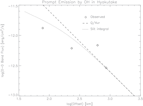
Figure 4. Flux of prompt emission. The diamonds are the observed flux (corrected for the unobserved R branch) of the rotationally hot portion, i.e., the prompt emission, of the 0-0 band of OH at each of the four positions of the slit, plotted as a function of offset from the nucleus, including differential refraction. The dashed line is simply the predicted radial profile of brightness, corresponding to the center of the slit. The dotted line is an integration over the area of the slit as discussed in the text.
Download figure:
Standard image High-resolution imageSince the projected distance from the nucleus varies significantly along the slit, our first correction is to do a proper integration over the slit at the various offsets. Equation (1) of A'Hearn & Millis (1984) for a slit centered on the nucleus is generalized in the appendix to a slit that is offset from the nucleus. That produces the dotted line in Figure 4. As expected it converges to the first calculation at large distances from the nucleus and it does approach the previous result for zero offset. The production rate was adjusted to  s−1 to normalize this dotted curve to the outermost observation. This is within the uncertainty quoted by Bockelée-Morvan et al. (1998), but uncertainties in the numerous other parameters can also contribute to the additional scaling.
The deviations from the dotted curve are quite clear. Some of this may be simply noise in the data, but at least a portion, probably the largest portion, of the deviations is due to physical effects that we have ignored. Although not directly measured, theoretical models, validated against observations at larger distance from the nucleus, suggest that the acceleration zone for the expansion of the gas extends out to order 100 km (Combi et al. 2005). The net effect of this would be to increase the signal in the zero-offset spectrum (which is actually offset by an estimated 78 km sunward due to atmospheric refraction) with respect to the observations at larger distances, the opposite of what we see. Optical depth is a larger effect. The prompt emission lines themselves are optically thin, but the inner coma is opaque to solar  . A very rough estimate is that the optical depth to solar
  in this uniform inner coma is 0.2 at 200 km and 2 at 20 km. Note that the closest edge of the slit to the nucleus is at a distance of about 34 km sunward. This may overestimate the optical depth somewhat since it ignores the Doppler shift of the expanding coma, but it indicates that optical depth is certainly a large factor in near-nucleus observations. The effect is certainly large enough to explain the lower flux at 2 arcsec and to offset the acceleration effect at 0 arcsec. The fact that the point at 7 arcsec is high could be due to poor SNR (this slit-position had relatively little exposure time) or it could be due to the fragment seen during this exposure or it could be due to temporal variability of the nuclear outgassing.
The fact that the points are consistent with an a priori calculation to within the uncertainties approaching a factor two in several of the many parameters of the calculations, strongly supports the conclusion that prompt emission after photo-dissociation is the dominant mechanism and that this prompt emission can be used to directly measure the water release by comets.
5. DISCUSSION
The prompt emission by OH in the near-UV provides an additional method of directly tracing the water production of comets, which complements the measurements of water itself (both in the near-infrared and in the submillimeter regime), the prompt emission of OH in the ground electronic state that is measured in the near-infrared, and the prompt emission of the red [O i] doublet in the visible. While measurement of daughter fragments of water (primarily of the OH near-UV fluorescence and of cometary  ) is still much easier, and thus much more common, than measuring the water directly, these methods all suffer from the need to model the photodissociation process of water, the excess energies of the various fragments, and the consequent averaging over the dissociation lifetime, limiting the temporal resolution of the inferred water release rate. The various examples of prompt emission after photodissociation all have complications compared to the direct measurement of water (opacity to the dissociating radiation, other sources or processes for the same prompt emission, uncertain branching rations that vary with solar activity, and so on). This indicates that a concerted effort to cross-calibrate the various prompt-emission mechanisms with a direct measurement of water by simultaneously observing an appropriate comet would significantly improve the accuracy of deduced water release rates. The near-IR prompt emission by OH has been cross-calibrated with water measurements by Bonev et al. (2004) using measurements of both species appearing in the same spectra, but a wider cross calibration effort, across different instruments and across the ultraviolet, visible, and infrared is ultimately needed.
It is important to note that our demonstration of prompt emission by photodissociation is for an active comet at 1 AU. The dominant processes may differ either for a very low activity comet or for a comet at a large heliocentric distance, which typically also implies low activity.
6. SUMMARY
We report the first spectrally resolved observation of prompt emission by cometary OH in the near-UV 0-0 band of the  –
– transition. These are among the strongest of the previously unidentified emission lines in the ultraviolet spectra of comets. Given the large uncertainties in many numerical parameters and noting the numerous physical processes that we have not included, the absolute flux is consistent with predictions assuming a production rate of water as deduced from other more traditional observations in the same period of time. Observations such as these can directly probe the release of water in the near-nuclear region of comets but we emphasize the fact that many parameters are not reliably known for any of the methods that use prompt emission.
The observations, data reduction, and some previous analyses of these spectra were supported by NASA's Planetary Astronomy Program through a grant to the University of Maryland. This analysis was supported by the University of Maryland and the individual authors. We thank the director and staff of Kitt Peak National Observatory for the opportunity to make these observations on very short notice. The observations were made while Meier was at UMd and the initial identification of the features was made while Krishna Swamy was a visitor at UMd. The manuscript was completed while A'Hearn was a Gauss Professor of the Göttingen Academy of Science. We acknowledge helpful discussions with Scott Budzien and others regarding the dissociation mechanism.
APPENDIX: INTEGRATION OVER SLIT
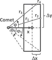
The simple radial profile proportional to 1/r can be integrated over the slit for an arbitrary offset. Assuming that the slit has half-width Δx and half-length Δy, with its center offset to (x, 0), i.e., parallel to the width of the slit, the integral of column density over the slit can be expressed as integrals over angles. We define  and
and  , as in Figure 5:

For  we get

while for  or for
  we get

Figure 5. Geometry of integration over the slit. The integration over (x, y) is converted into an integral over (r, ϕ), which can be evaluated analytically.
Download figure:
Standard image High-resolution image
We can then express the ratio, η, of the integral over the aperture to the value at the center of the aperture multiplied by the area of the aperture as
where A = x/(2 ΔxΔy). For our aperture this converges to unity within 1% by 1300 km and as  , it converges to the value given by A'Hearn & Millis's (1984) equation.