


ABSTRACT
We present photometry for an unprecedented database of some 5.5 million stars distributed throughout the Large Magellanic Cloud main body, from 21 fields covering a total area of 7.6 deg2, obtained from Washington CT1T2 CTIO 4 m MOSAIC data. Extensive artificial star tests over the whole mosaic image data set and the observed behavior of the photometric errors with magnitude demonstrate the accuracy of the morphology and clearly delineate the position of the main features in the color–magnitude diagrams (CMDs). The representative T1(MS TO) mags are on average ∼0.5 mag brighter than the T1 mags for the 100% completeness level of the respective field, allowing us to derive an accurate age estimate. We have analyzed the CMD Hess diagrams and used the peaks in star counts at the main sequence turnoff and red clump (RC) locations to age date the most dominant sub-population (or "representative" population) in the stellar population mix. The metallicity of this representative population is estimated from the locus of the most populous red giant branch track. We use these results to derive age and metallicity estimates for all of our fields. The analyzed fields span age and metallicity ranges covering most of the galaxy's lifetime and chemical enrichment, i.e., ages and metallicities between ∼1 and 13 Gyr and ∼−0.2 and −1.2 dex, respectively. We show that the dispersions associated with the mean ages and metallicities represent in general a satisfactory estimate of the age/metallicity spread (∼1–3 Gyr/0.2–0.3 dex), although a few subfields have a slightly larger age/metallicity spread. Finally, we revisit the study of the vertical structure (VS) phenomenon, a striking feature composed of stars that extend from the bottom, bluest end of the RC to ∼0.45 mag fainter. We confirm that the VS phenomenon is not clearly seen in most of the studied fields and suggest that its occurrence is linked to some other condition(s) in addition to the appropriate age, metallicity, and the necessary red giant star density.
Export citation and abstract BibTeX RIS
1. INTRODUCTION
The relative proximity of the Large Magellanic Cloud (LMC) and the advent of wide field mosaic CCD detectors have stimulated a variety of photometric surveys aimed at improving our knowledge of the structure, extent, star formation history (SFH), and age–metallicity relationship (AMR) of our galactic neighbor.
To our knowledge, Subramanian & Subramanian (2010) sum up previous efforts and contribute with their own work on LMC structure. They used the red clump (RC) stars from the VI photometric data of the Optical Gravitational Lensing Experiment (OGLE III; Udalski et al. 2008) survey and from the Magellanic Cloud Photometric Survey (MCPS; Zaritsky et al. 2004) to estimate the structural parameters of the LMC disk, namely, the inclination i and the position angle of the line of nodes P.A.lon(ϕ). Their results are comparable with most previous estimates. They also found that the choice of center has a negligible effect on the estimated parameters. In addition, Saha et al. (2010) have performed a thorough analysis of the LMC outer limits based on a National Optical Astronomy Observatory (NOAO) survey designed to detect, map, and characterize the extended structure of the Magellanic Clouds (MCs). From photometry of 80 6 × 06 fields located at radii of 7° to 19° north of the LMC bar, they found main-sequence (MS) stars associated with the LMC out to 16° from the center, while the much rarer giants can only be convincingly detected out to 11°. They did not rule out the possible existence of a stellar halo, which they show may only begin to dominate over the disk at still larger radii than where they have detected LMC populations.
With respect to the LMC's SFH and AMR, there exist two studies—based on photometric surveys—most worthy of mention, since they summarize our current knowledge in this field. First, Harris & Zaritsky (2009) presented the first-ever global, spatially resolved reconstruction of the SFH, based on the application of their StarFISH analysis software to the multiband photometry of twenty million stars from the UBVI MCPS. They found that there existed a long quiescent epoch (from ∼12 to 5 Gyr ago) during which the star formation was suppressed throughout the LMC; the metallicity also remained stagnant during this era. They also claimed that cluster and field AMRs are tightly coupled, although their Figure 20 does not show such a strong connection. Second, Rubele et al. (2012) presented the first results from the VISTA near-infrared YJKs survey of the Magellanic system (VMC; Cioni et al. 2011) based on four tiles in the LMC, covering a total area of ∼45. Their data clearly reveal the presence of peaks in the star formation rate, SFR(t), at ages log(t/yr) 9.3 and 9.7, which appear in most of the subregions. The most recent SFR(t) was found to vary greatly from subregion to subregion, whereas the AMRs, instead, turned out to be remarkably similar across the LMC.
This paper is aimed at presenting new Washington CT1T2 photometry of the LMC main body which goes deeper than the MCPS survey (Harris & Zaritsky 2009) and covers ≈1.7 times the currently available VMC survey area (Rubele et al. 2012). Harris & Zaritsky did not go deep enough to derive the full SFH for the oldest populations from the information on the MS. They reached a limiting magnitude between V = 20 and V = 21 mag, depending on the local degree of crowding in the images, corresponding to stars younger than 3 Gyr old on the MS (Noel et al. 2009). This could be the reason why they did not find a satisfactory match between their field AMR and that of clusters younger than ∼12 Gyr, besides the fact that the ages and metallicities for the 85 clusters used in the comparisons are not themselves on a homogeneous scale or on the same field age/metallicity scale. Saha et al. (2010) used the same telescope, instrument setup, and filters as for the present data set, but they explored the very outer region of the LMC, so that its main body was not surveyed. Finally, Rubele et al.'s results are based on a photometric data set whose limiting Ks mag for a 100% completeness level barely reaches two magnitudes below the RC. In our case, the T1 mag for 100% completeness level reaches between ∼3.5 and 4.5 mag below the RC. Other advantages of the present data set are that the Washington CT1 system standard giant branch (SGB) technique is found to have three times the metallicity sensitivity of the analogous VI technique (Geisler & Sarajedini 1999). Thus, for a given photometric accuracy, metallicities can be determined three times more precisely with the Washington technique. In addition, the ability of the Washington system to estimate ages of star clusters has long been proven (Piatti et al. 2011a and references therein). From the δT1 index, calculated by determining the difference in the T1 magnitude of the RC and the MS turnoff (TO; Geisler et al. 1997), ages older than ∼1 Gyr can be estimated with typical errors of 10% (Piatti 2012). This yields a unique and powerful tool in which ages and metallicities for both clusters and star fields are determined homogeneously.
Given these advantages, we set out to obtain a large, deep, and homogeneous database of LMC field and cluster star photometry in order to investigate the SFH, AMR, metallicity distribution, metallicity gradient, constrain times of starbursts, etc. Here, we concentrate on presenting the main photometric results of the field stars. Other papers will present the analysis of the field stars and the cluster results.
The paper is organized as follows: Section 2 describes the data handling, putting special emphasis on performing extensive artificial star tests to determine photometric errors and completeness (Section 2.1) and in producing color–magnitude diagrams and Hess diagrams of the same (Section 2.2). Section 3 deals with global properties of the color–magnitude diagrams (CMDs), such as the MS luminosity function (LF, Section 3.1) and the derivation of the mean mag of the RC (Section 3.2). In Section 4, we determine the age and metallicity of the most numerous stellar population in the studied LMC fields, and in Section 5 we revisit the vertical structure (VS) phenomenon, observationally discovered by Piatti et al. (1999). Finally, Section 6 summarizes our results.
2. DATA HANDLING
Our goal was to cover a wide area of the LMC with fields dominated by significant LMC populations but avoiding the crowded central regions. The fields were centered either on star clusters of interest or fields judged to possess a significant number of stars in the range of age and metallicity in which the VS phenomenon should be activated (Girardi 1999). We obtained images at the Cerro-Tololo Inter-American Observatory (CTIO) 4 m Blanco telescope with the Mosaic II camera (36' × 36' field with an 8 K × 8 K CCD detector array) covering 21 fields of the LMC main body for a total area of ∼7.6 deg2. The log of the observations is presented in Table 1, where the main astrometric, photometric, and observational information is summarized. Only a single image was taken in each filter, as we judged that the dynamic range required to suit our science goals could be met most efficiently this way. Some fields have shorter exposure times simply due to time constraints. Figure 1 depicts the spatial distribution of the LMC fields, represented by yellow numbered boxes. The maximum deprojected distance probed from the center of the LMC is ∼7.5 deg. For comparison purposes, we schematically included the regions encompassed by different photometric surveys, namely, MCPS (Harris & Zaritsky 2009, blue), OGLE III (Udalski et al. 2008, red), and VMC (Rubele et al. 2012, magenta).
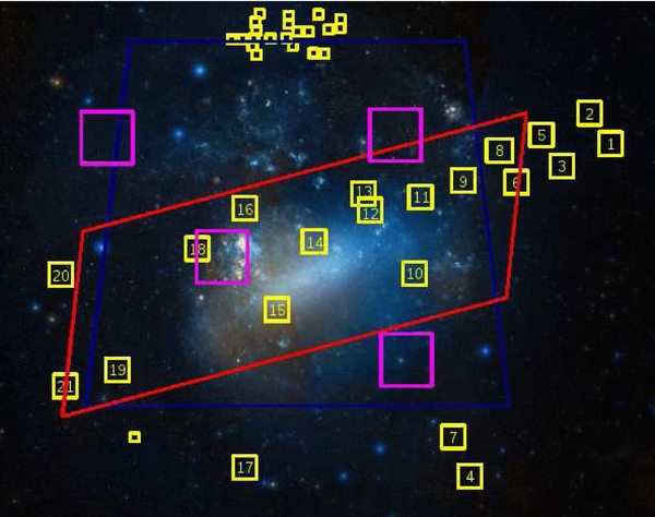
Figure 1. Spatial distribution of the presently studied LMC star fields (numbered yellow boxes) overplotted on a image downloaded from the DSS2 All Sky Survey via Wikisky (http://www.wikisky.org/). The small yellow boxes represent the fields studied by Piatti et al. 1999 (see their Figure 1 and the present Section 5 for details). Schematic regions encompassed by MCPS (Harris & Zaritsky 2009, blue), OGLE III (Udalski et al. 2008, red), and VMC (Rubele et al. 2012, magenta) are also superimposed.
Download figure:
Standard image High-resolution imageTable 1. Star Fields in the LMC
| Field | α2000 | δ2000 | l | b | E(B − V) | Date | Exposure | Airmass | Seeing |
|---|---|---|---|---|---|---|---|---|---|
| Designation | (h m s) | (° ' '') | (°) | (°) | (mag) | C R I (sec) | C R I | C R I ('') | |
| 1 | 04 23 08.41 | −66 29 32.7 | 278.68 | −39.20 | 0.01 ± 0.01 | 2008 Dec 20 | 500 120 120 | 1.281 1.274 1.278 | 1.2 0.8 0.8 |
| 2 | 04 28 45.27 | −65 43 23.8 | 277.48 | −38.97 | 0.01 ± 0.01 | 2008 Dec 20 | 500 120 120 | 1.285 1.276 1.280 | 1.2 0.9 1.0 |
| 3 | 04 31 11.35 | −67 03 33.0 | 278.95 | −38.25 | 0.02 ± 0.01 | 2008 Dec 20 | 500 120 120 | 1.326 1.315 1.320 | 1.1 1.0 0.8 |
| 4 | 04 32 31.11 | −74 59 55.5 | 287.90 | −34.86 | 0.09 ± 0.01 | 2008 Dec 19 | 1200 180 180 | 1.426 1.421 1.423 | 1.1 0.8 0.8 |
| 5 | 04 36 40.92 | −66 16 26.4 | 277.77 | −38.03 | 0.01 ± 0.01 | 2008 Dec 20 | 500 120 120 | 1.389 1.373 1.381 | 1.2 1.0 0.9 |
| 6 | 04 39 17.96 | −67 28 35.4 | 279.09 | −37.37 | 0.04 ± 0.01 | 2008 Dec 20 | 500 120 120 | 1.440 1.423 1.432 | 1.3 1.0 0.9 |
| 7 | 04 40 01.09 | −73 59 56.6 | 286.54 | −34.84 | 0.09 ± 0.01 | 2008 Dec 19 | 1200 180 180 | 1.421 1.414 1.417 | 1.0 0.9 0.7 |
| 8 | 04 44 12.27 | −66 40 18.7 | 277.94 | −37.19 | 0.02 ± 0.01 | 2008 Dec 20 | 500 120 120 | 1.485 1.446 1.455 | 1.1 1.0 0.7 |
| 9 | 04 49 50.84 | −67 26 32.3 | 278.64 | −36.43 | 0.04 ± 0.01 | 2008 Dec 20 | 500 120 120 | 1.512 1.490 1.501 | 1.3 1.0 0.9 |
| 10 | 04 57 01.32 | −69 48 37.1 | 281.19 | −35.10 | 0.11 ± 0.01 | 2008 Dec 18 | 1500 300 300 | 1.302 1.299 1.300 | 1.4 1.2 1.0 |
| 11 | 04 57 52.29 | −67 51 43.8 | 278.87 | −35.58 | 0.06 ± 0.01 | 2008 Dec 20 | 500 120 120 | 1.549 1.526 1.537 | 1.2 1.1 0.9 |
| 12 | 05 07 49.38 | −68 11 21.4 | 278.97 | −34.59 | 0.06 ± 0.01 | 2008 Dec 20 | 500 120 120 | 1.581 1.557 1.569 | 1.0 0.9 0.9 |
| 13 | 05 09 23.97 | −67 46 40.3 | 278.45 | −34.54 | 0.06 ± 0.01 | 2008 Dec 18 | 1200 180 180 | 1.279 1.273 1.276 | 1.4 1.2 1.0 |
| 14 | 05 19 02.70 | −68 59 59.2 | 279.66 | −33.42 | 0.08 ± 0.01 | 2008 Dec 18 | 1200 180 180 | 1.403 1.385 1.394 | 1.4 1.0 0.9 |
| 15 | 05 27 17.84 | −70 44 08.2 | 281.54 | −32.40 | 0.08 ± 0.01 | 2008 Dec 18 | 1200 180 180 | 1.475 1.457 1.456 | 1.4 1.0 1.0 |
| 16 | 05 33 21.19 | −68 09 08.6 | 278.42 | −32.26 | 0.06 ± 0.01 | 2008 Dec 18 | 1200 180 180 | 1.497 1.474 1.485 | 1.4 1.0 0.9 |
| 17 | 05 37 48.36 | −74 46 59.9 | 286.05 | −30.91 | 0.11 ± 0.01 | 2008 Dec 19 | 1200 180 180 | 1.447 1.439 1.443 | 1.0 0.8 0.7 |
| 18 | 05 43 56.31 | −69 10 48.1 | 279.50 | −31.20 | 0.06 ± 0.01 | 2008 Dec 19 | 1200 180 180 | 1.368 1.355 1.362 | 1.0 0.8 0.7 |
| 19 | 06 07 15.77 | −72 16 32.1 | 282.93 | −29.09 | 0.11 ± 0.01 | 2008 Dec 19 | 1200 180 180 | 1.437 1.424 1.430 | 1.1 0.8 0.8 |
| 20 | 06 14 28.07 | −69 50 52.2 | 280.16 | −28.51 | 0.10 ± 0.01 | 2008 Dec 18 | 1200 180 180 | 1.318 1.311 1.314 | 1.1 0.9 0.9 |
| 21 | 06 20 06.93 | −72 44 16.6 | 283.46 | −28.12 | 0.08 ± 0.01 | 2008 Dec 19 | 1200 180 180 | 1.482 1.466 1.474 | 1.0 0.9 0.8 |
Download table as: ASCIITypeset image
The data reduction followed the procedures documented by the NOAO Deep Wide Field Survey team (Jannuzi et al. 2003) and utilized the mscred package in IRAF.3 We performed overscan, trimming and cross-talk corrections, bias subtraction, obtained an updated world coordinate system (WCS) database, flattened all data images, etc., once the calibration frames (zeros, sky and dome flats, etc.) were properly combined.
Nearly 90 independent magnitude measures of standard stars from the list of Geisler (1996) were also derived per filter for each night using the apphot task within IRAF, in order to secure the transformation from the instrumental to the Washington CT1T2 standard system. The standard fields SA 92, 98, 101, PG 0231+51, and NGC 3680 contain between 8 and 14 standard stars each distributed over an area similar to that of the Mosaic II camera, so that we measured magnitudes of standard stars in each of its eight chips. The relationships between instrumental and standard magnitudes were obtained by fitting the equations:


where ai, bi, and ci (i = 1, 2, and 3) are the fitted coefficients, and X represents the effective airmass. Capital and lowercase letters represent standard and instrumental magnitudes, respectively. Here, we use lower case r and i for the T1 and T2 filters because we in fact used RI(KC) filters as more efficient substitutes, as shown by Geisler (1996), but our final standard system is that of the Washington CT1T2 system. We solved the transformation equations with the fitparams task in IRAF for each night, and for the eight chips simultaneously, and found mean zero points of −0.028 ± 0.017(σ) in c, −0.709 ± 0.003 in r, and −0.039 ± 0.007 in i, and mean color terms of −0.092 ± 0.004 in c, −0.021 ± 0.001 in r, and 0.060 ± 0.005 in i for the three nights. We then substituted these mean zero point and color term values into the above equations and solved for the airmass coefficient for each night. Typical values were 0.308, 0.095, and 0.064 for c, r, and i, respectively. The nightly rms errors from the transformation to the standard system were 0.021, 0.023, and 0.017 mag for C, T1, and T2, respectively, indicating that these nights were of excellent photometric quality.
The stellar photometry was performed using the star-finding and point-spread-function (PSF) fitting routines in the daophot/allstar suite of programs (Stetson et al. 1990). We measured magnitudes on the single image created by joining all eight chips together using the updated WCS. This allowed us to use a unique reference coordinate system for each LMC field. For each Mosaic image, a quadratically varying PSF was derived by fitting ∼960 stars (nearly 100–120 stars per chip), once the neighbors were eliminated using a preliminary PSF derived from the brightest, least contaminated ∼240 stars (nearly 30–40 stars per chip). Both groups of PSF stars were interactively selected. We then used the allstar program to apply the resulting PSF to the identified stellar objects and to create a subtracted image which was used to find and measure magnitudes of additional fainter stars. This procedure was repeated three times for each frame. After deriving the photometry for all detected objects in each filter, a cut was made on the basis of the parameters returned by DAOPHOT. Only objects with χ < 2, photometric error less than 2σ above the mean error at a given magnitude, and |SHARP| < 0.5 were kept in each filter (typically discarding about 10% of the objects), and then the remaining objects in the C and T1 lists were matched with a tolerance of 1 pixel and raw photometry obtained. We computed aperture corrections from the comparison of PSF and aperture magnitudes by using the neighbor-subtracted PSF star sample. The resulting aperture corrections were on average less than 0.02 mag (absolute value) for c, r, and i images, respectively. Finally, we standardized the resulting instrumental magnitudes and combined all the independent measurements using the stand-alone daomatch and daomaster programs, kindly provided by Peter Stetson. The final information for each field consists of a running number per star, its R.A. and decl. coordinates, the measured T1 magnitudes and C − T1 and T1 − T2 colors, and the observational errors σ(T1), σ(C − T1), and σ(T1 − T2) as provided by daophot/allstar routines. Note that T1 − T2 colors were included in this paper for completeness purposes, since they are thought to be useful for breaking the age–metallicity degeneracy when studying the LMC AMR, which will be the subject of a forthcoming paper. Table 2 gives this information for Field 1. Only a portion of this table is shown here for guidance regarding its form and content. The whole content of Table 2, as well as the final information for the remaining fields, is available in the online version of the journal. For the subsequent analysis, we subdivided each 36' × 36' field into 16 uniform 2 K × 2 K regions (9' × 9') in order to deal with comparable-sized individual areas to Harris & Zaritsky (2009) and Rubele et al. (2012). We labeled such subfields with letters A to P moving from the west to the east and from the south to the north (see the Appendix, Figure 8).
Table 2. CT1 Data of Stars in the Field 1
| Star | R.A. | Decl. | T1 | σ(T1) | C − T1 | σ(C − T1) | T1 − T2 | σ(T1 − T2) |
|---|---|---|---|---|---|---|---|---|
| (deg) | (deg) | (mag) | (mag) | (mag) | (mag) | (mag) | (mag) | |
| ... | ... | ... | ... | ... | ... | ... | ... | ... |
| 304 | 65.16796 | −66.75647 | 21.557 | 0.084 | 2.688 | 0.151 | 0.706 | 0.122 |
| 305 | 65.25958 | −66.75709 | 21.488 | 0.020 | 0.623 | 0.030 | 0.369 | 0.041 |
| 306 | 65.02176 | −66.75481 | 22.445 | 0.052 | 0.855 | 0.075 | 0.389 | 0.088 |
| ... | ... | ... | ... | ... | ... | ... | ... |
Only a portion of this table is shown here to demonstrate its form and content. Machine-readable and Virtual Observatory (VO) versions of the full table are available.
Download table as: Machine-readable (MRT)Virtual Observatory (VOT)Typeset image
2.1. Photometric Errors, Limiting Magnitudes, and Completeness Tests
As is well known, photometric errors, crowding effects, and the detection limit of the images cause incompleteness and therefore results in the increasing loss of stars at fainter magnitudes. Commonly, artificial star tests on the deepest images are performed in order to derive the completeness level at different magnitudes. However, since our data set includes a variety of exposure times, airmasses, crowding levels, etc., we prefer to perform artificial star tests over the whole image data set. This method consumes much more time, but we gain a detailed knowledge of the quality and the scope of the data in the analysis of each image. This is also the best way to assess real photometric errors.
We used the stand-alone addstar program in the daophot package (Stetson et al. 1990) to add synthetic stars, generated at random with respect to position and magnitude, to each image in order to derive its completeness level. We added a number of stars equivalent to ∼5% of the measured stars in order to avoid in the synthetic images significantly more crowding than in the original images. On the other hand, to avoid small number statistics in the artificial-star analysis, we created five different images for each original one. We used the option of entering the number of photons per ADU in order to properly add the Poisson noise to the star images.
We then repeated the same steps to obtain the photometry of the synthetic images as described above, i.e., performing three passes with the daophot/allstar routines. The errors and star-finding efficiency were estimated by comparing the output and the input data for these stars using the daomatch and daomaster tasks. We plotted in Figure 2 the resultant completeness fractions as a function of magnitude for each field. Figure 2 shows that the 50% completeness level is located at C ∼ 23.5–24.5 and T1 ∼ 23.0–24.0, depending on the crowding and exposure time. In the subsequent analysis, we only analyzed data for each field to the magnitude where the completeness level begins to fall below 100%. For completeness purposes, we include in Table 7 (see the Appendix) the mean values of the C and T1 magnitudes reached at a 50% completeness level for the 21 studied LMC fields. They were extracted from Figure 2. We also include a comparison between the photometry for stars measured in both Fields 12 and 13 (see the Appendix, Figure 9).

Figure 2. Completeness curves for the C and T1 filters obtained from artificial star tests performed as described in Section 2.1.
Download figure:
Standard image High-resolution image2.2. Color–Magnitude and Hess Diagrams
In Figure 3, we plot a series of multi-panel graphics containing photometry for each LMC field. First of all, the CMDs for all measured stars are depicted in the top left panels. We measured from ∼22 up to 660 thousand stars per field, with an average of ∼258 thousand stars, thus yielding an unprecedented CT1T2 photometric database of some ∼5.5 million stars. In this statistic, we include cluster stars spread over the 21 LMC fields. We found between 1 to 60 star clusters per field, with an average of 10. Note that it was not necessary to mask out cluster stars since they result in a negligible fraction of the total stars in each field (≪ 0.1%). The CMDs are powerful tools to estimate, with the aid of empirical calibrations and/or theoretical isochrones, the ranges of age, metallicity, and stellar mass of each observed LMC region. They can also be fruitfully used to estimate the values of the interstellar reddenings across the fields and their mean distances. We will treat these parameters in detail in a forthcoming paper.

Figure 3.
C − T1 vs. T1 diagram for the stars measured in Field 1 (top left panel). The photometric errors σ(T1) and σ(C − T1) (top right panel), the Hess diagram (bottom left panel), and the both obtained normalized and differential MS LFs for the J subfield (bottom right panel) are also shown. The Hess diagram has also superimposed lines which indicate the 50% and 100% completeness levels. (The complete figure set (21 images) is available in the online journal.)
Download figure:
Standard image High-resolution imageThe top right panels show the behavior of the photometric errors σ(T1) and σ(C − T1) (from the allstar internal errors)—expressed in magnitudes—against their corresponding T1 magnitudes. As can be seen, it would seem that a relatively small dispersion accompanies the expected tendency of increasing errors as the magnitude increases along ∼9 mag. Given this behavior and the small photometric errors involved to well below the MS TO in each field, we are confident that our subsequent analysis will yield accurate morphology and position of the main features in the CMDs. For example, σ(C − T1) is ∼0.2 mag at T1 ∼ 23, which is smaller than the observed width of the MS at this T1 magnitude level. Note also that when performing artificial star tests we recovered photometric errors which follow the same trend as those in Figure 3 (top right panels), since we applied the same procedure to perform the photometry in both sorts of images—with and without artificial stars added—and a number of stars equivalent to only ∼5% of the measured stars were added in order to avoid significantly more crowding in the synthetic images than in the original images.
For many years, Hess diagrams have played an increasingly prominent role in the analysis of photometric data, in particular of the Magellanic Clouds. They show the frequency or density of occurrence of stars at various positions on the CMD, thus providing a star density map in the CMD. Hess diagrams have been profitably exploited by using different robust techniques (Harris & Zaritsky 2001; Dolphin 2002, and references therein). Here, we simply take advantage of Hess diagrams to identify the prevailing CMD features—in terms of density of stars—and their intrinsic dispersions, MS LFs, etc. In order to produce these Hess diagrams we counted the number of stars placed in different magnitude–color bins with sizes [ΔT1, Δ(C − T1)] = (0.1, 0.05) mag and then we represented the resultant count scales with a 10 gray level logarithmic scale. The resultant Hess diagrams are depicted in the bottom left panels of Figure 3.
The MS LFs were obtained by counting the number of stars in T1 bins of 0.25 mag along the MSs. The chosen bin size encompasses the T1 magnitude errors of the stars in each bin, thus producing an appropriate sample of the stars. Note that typical photometric T1 errors for most of the measured stars are ≲0.20 mag. As is well known, the bin size should be of the order of the uncertainties of the quantity involved to best represent an intrinsic distribution of such a quantity (Piatti 2010; Piatti et al. 2011a, 2011b). Furthermore, the LFs have only been computed for T1 magnitudes where 100% completeness levels are reached (see Section 2.1), and then they were normalized. This means—statistically speaking—that the shape of these LFs are not driven by the chosen bin size or incompleteness effects. The LFs show the intrinsic variation in the number of stars along the MS. The C − T1 color boundaries of the MSs were defined taking as reference the placement in the Hess diagrams of theoretical zero-age main sequences (ZAMSs) for metallicities more metal-poor than [Fe/H] ∼ −0.3 dex (Girardi et al. 2002), as well as the photometric errors. We first reddened the ZAMSs with E(B − V) values between 0.00 and ≲0.20 mag (Cole et al. 2005; Subramanian & Subramanian 2010) in order to embrace any position of them along the color axis, and shifted them according to the LMC true distance modulus m − M = 18.50 ± 0.10 mag (Glatt et al. 2010), and then superimposed them on the observed Hess diagrams. We illustrate the MS LFs derived for the J subfield of each image—expressed in normalized star count units—in the bottom right panels of Figure 3.
3. GLOBAL CMD PROPERTIES
3.1. Main-sequence Luminosity Functions
The CMDs of the 21 observed LMC fields (upper left panels of Figure 3) exhibit different features which tell us about the stellar populations of this galaxy. A mixture of young through old stellar populations clearly appears to be the main feature of these CMDs. Note that fields with an important presence of younger populations have MSs which extend more than 8 mag in T1, whereas those of predominant older populations have MSs with still some 3 mag of extension. Other obvious traits presented in all the fields are the populous and broad subgiant branches—an indicator of the evolution of stars with ages (masses) within a non-negligible range—the RCs and the red giant branches (RGBs). The RC is somewhat elongated/tilted in Fields 9, 16, and 18, evidence for differential reddening, while there is an apparent gap below it in Field 2. RCs also appear to be populated at brighter magnitudes by the so-called vertical RC structure (Zaritsky & Lin 1997; Gallart 1998; Ibata et al. 1998). However, there is no clear existing evidence of the VS stars, extending to fainter mags from the blue end of the RC, seen in some LMC fields (Piatti et al. 1999), except, perhaps, for Field 21.
Since the LMC field CMDs are obviously composed of MS stars of different stellar populations, we assume that the observed MS in each field is a result of the superposition of MSs with different TOs (ages) and constant LFs. We also assume, for simplicity, the same metallicity for all MS stars within a given subfield. Hence, the difference between the number of stars of two adjacent magnitude intervals gives the intrinsic number of stars belonging to the faintest interval. Consequently, the biggest difference is directly related to the most populated TO, as illustrated by the differential LFs of Figure 3 (see bottom right panels). We refer to these TOs of the most numerous stellar population as "representative" TOs along the line of sight. This was defined by Geisler et al. (2003) and subsequently used by Piatti et al. (2003a, 2003b, 2007) and Piatti (2012), among others. The definition of a representative TO could not converge to any dominant TO (age) value if the stars in a given field came from a constant SFR integrated over all time. In such a case, the difference between the number of stars of two adjacent magnitude intervals would result in the same value for any T1 bin. For our fields, however, we could clearly identify the respective most populated TOs. The resultant representative T1(MS TO) mags are in average ∼0.5 mag brighter than the T1 mags for the 100% completeness level of the respective field, i.e., the faintest T1 mag where completeness is still 100%. Therefore, we actually reach the MS TO of the representative population of each field with a negligible loss of stars at that magnitude.
The prevailing TOs are typically ∼25%–50% more populous than the next most dominant population, represented by a secondary peak—sometimes there even exists a third peak—in the differential LFs (see bottom right panels of Figure 3). Again, these peaks are real since the differential LFs have been obtained from LFs computed for T1 mag regions where completeness levels are 100%. In order to take into account the presence of a secondary peak, or a slightly broader T1 mag distribution in the differential LFs around the representative TO, we assigned to the MS TO T1 magnitudes dispersions four times those typical of the photometry at the TO level, i.e., 〈σ(T1)〉 ≈ 0.05 mag. In general, this should be a satisfactory estimate of the T1 mag spread around the prevailing population T1 mag, although a few individual subfields show a slightly larger representative T1 mag spread. Table 3 lists the adopted mean values of the reddening corrected T1o magnitude for the representative MS TOs. Note that the differential LFs in the bottom right panels of Figure 3 do not necessarily represent the behavior of each subfield in the respective observed LMC regions, since we chose to show only the J subfield for illustrative purposes. As for the interstellar extinction of MS stars, we measured field reddening values for each one of the 336 subfields by interpolating the extinction maps of Burstein & Heiles (1982), and then averaged these values for each of the 21 selected LMC fields. The resulting mean E(B − V) values are listed in Column 6 of Table 1. Our calculations show that it is reasonable to assume uniform reddening within each subfield. However, as we pointed out above, Fields 9, 16, and 18 show somewhat elongated/tilted RCs, evidence for differential reddening. It is probable that the spatial resolution of the Burstein & Heiles (1982)'s maps does not allow us to detect such a relatively small amount of differential extinction.
Table 3. Mean Reddening Corrected T1o Values (in mag) for the Representative MS Populations in LMC Fields
| Field | A | B | C | D | E | F | G | H | I | J | K | L | M | N | O | P |
|---|---|---|---|---|---|---|---|---|---|---|---|---|---|---|---|---|
| 1 | 22.125 | 22.375 | 22.375 | 22.125 | 21.625 | 21.875 | 21.875 | 21.875 | 22.125 | 22.375 | 21.875 | 21.875 | 21.625 | 21.875 | 22.125 | 21.875 |
| 2 | 21.875 | 22.375 | 21.875 | 21.875 | 22.125 | 21.875 | 21.875 | 21.625 | 21.875 | 22.125 | 21.875 | 21.875 | 21.875 | 22.125 | 21.625 | 21.625 |
| 3 | 22.125 | 21.875 | 21.625 | 21.875 | 22.125 | 21.875 | 21.875 | 21.625 | 21.875 | 21.875 | 21.625 | 21.875 | 21.625 | 21.625 | 21.875 | 21.625 |
| 4 | 22.125 | 21.875 | 21.875 | 21.875 | 21.875 | 22.625 | 21.875 | 21.875 | 21.875 | 21.875 | 21.875 | 21.875 | 22.125 | 22.125 | 21.625 | 21.625 |
| 5 | 22.125 | 21.875 | 21.875 | 21.875 | 21.875 | 21.875 | 21.625 | 21.875 | 21.875 | 21.875 | 21.625 | 22.125 | 22.125 | 21.875 | 22.125 | 21.625 |
| 6 | 21.625 | 21.625 | 21.625 | 21.625 | 21.875 | 21.625 | 21.875 | 21.625 | 21.625 | 21.625 | 21.875 | 21.625 | 21.625 | 21.875 | 21.625 | 21.625 |
| 7 | 21.875 | 21.875 | 21.125 | 21.875 | 21.875 | 21.875 | 21.625 | 21.625 | 21.875 | 21.875 | 22.125 | 21.875 | 22.125 | 21.625 | 21.625 | 21.875 |
| 8 | 21.625 | 21.875 | 21.625 | 21.625 | 21.625 | 21.875 | 21.625 | 21.625 | 21.625 | 21.625 | 21.625 | 21.625 | 21.375 | 21.375 | 21.625 | 21.625 |
| 9 | 21.375 | 21.375 | 21.125 | 21.125 | 21.625 | 21.125 | 20.875 | 21.125 | 21.375 | 21.625 | 21.375 | 21.125 | 21.625 | 21.375 | 21.125 | 21.375 |
| 10 | 20.625 | 20.375 | 20.875 | 20.625 | 20.875 | 20.375 | 20.375 | 20.375 | 20.375 | 20.375 | 20.625 | 20.375 | 20.625 | 20.625 | 20.125 | 20.375 |
| 11 | 20.625 | 21.125 | 20.875 | 21.125 | 20.875 | 20.625 | 21.125 | 21.125 | 21.125 | 21.375 | 20.875 | 21.125 | 20.875 | 21.125 | 20.875 | 21.125 |
| 12 | 20.625 | 20.875 | 20.875 | 20.625 | 21.125 | 21.125 | 20.875 | 21.125 | 20.875 | 20.875 | 21.125 | 20.625 | 20.875 | 20.875 | 20.875 | 21.125 |
| 13 | 20.625 | 20.625 | 20.625 | 20.625 | 20.625 | 20.875 | 20.875 | 20.875 | 20.875 | 21.125 | 20.875 | 20.875 | 20.375 | 20.875 | 20.625 | 20.875 |
| 14 | 20.125 | 19.875 | 19.875 | 20.125 | 19.675 | 19.675 | 20.125 | 20.375 | 19.875 | 19.675 | 20.375 | 20.875 | 20.875 | 20.675 | 20.875 | 20.875 |
| 15 | 20.875 | 21.125 | 20.875 | 20.875 | 21.125 | 20.875 | 20.875 | 20.875 | 20.875 | 20.875 | 20.875 | 20.675 | 20.875 | 20.675 | 20.625 | 20.375 |
| 16 | 21.375 | 21.125 | 21.125 | 21.125 | 21.375 | 21.125 | 21.375 | 21.375 | 21.125 | 21.375 | 21.375 | 20.875 | 21.125 | 21.375 | 21.125 | 20.875 |
| 17 | 21.375 | 21.375 | 21.875 | 21.875 | 21.875 | 21.675 | 21.675 | 21.375 | 21.675 | 21.875 | 21.875 | 21.675 | 21.675 | 21.675 | 21.675 | 21.675 |
| 18 | 21.125 | 21.375 | 21.675 | 21.675 | 21.125 | 21.675 | 21.675 | 21.875 | 21.125 | 21.125 | 21.375 | 21.875 | 20.875 | 21.375 | 21.375 | 21.125 |
| 19 | 21.675 | 21.875 | 21.375 | 21.875 | 21.625 | 21.875 | 21.625 | 21.625 | 21.625 | 21.625 | 21.625 | 21.625 | 21.625 | 21.375 | 21.875 | 21.625 |
| 20 | 21.625 | 21.875 | 21.625 | 21.625 | 21.625 | 21.625 | 21.875 | 21.625 | 21.625 | 21.875 | 21.375 | 21.875 | 21.625 | 21.625 | 21.375 | 21.375 |
| 21 | 21.625 | 21.875 | 21.625 | 21.625 | 21.875 | 21.875 | 21.875 | 21.875 | 21.625 | 21.875 | 21.625 | 21.875 | 21.625 | 21.625 | 21.875 | 21.625 |
Download table as: ASCIITypeset image
3.2. Red Clumps
RC stars are usually used as standard candles for distance determinations (Paczynski & Stanek 1998; Olsen & Salyk 2002; Subramaniam 2003). However, they are also often used in age estimates based on the magnitude difference δ between the clump/HB and the TO for intermediate-age and old clusters (see, e.g., Phelps et al. 1994), since the RC mag is relatively invariant to population effects such as age and metallicity for such stars (e.g., Subramanian & Subramanian 2010). Since the TO magnitude is an excellent age indicator, so also are δ(V), δ(R), and δ(T1) (see Section 4). Here, we study the RCs of our LMC fields, assuming that the peak of the T1(RC) mag distribution corresponds to the most populous T1(MSTO) in the respective field, although, again, this value should vary little with age or metallicity.
We first defined the rectangular region in the Hess diagram that encompasses the RC observed in each field. Then, we built T1 histograms for these RC stars using intervals of Δ(T1) = 0.10 mag, and finally we performed Gaussian fits to derive the mean values and the FWHMs of the T1(RC) distributions. We performed Gaussian fits using the ngaussfit routine of the IRAF stsdas package. We adopted a single Gaussian, and fixed the constant and linear terms to the corresponding background levels and to zero, respectively. The center of the Gaussian, its amplitude, and its FWHM acted as variables. We iterated the fitting procedure once on average, after eliminating a couple of discrepant points. T1(RC) mags were finally determined with a standard deviation of ± 0.01 mag in all cases. The FWHMs are in general of the order of ten times that typical of the photometry at the RC level, i.e., 〈σ(T1)〉 ≈ 0.02 mag, showing that population effects are not negligible. Figure 4 shows the T1(RC) histograms, previously normalized, and the fitted Gaussians superimposed, while Table 4 lists the adopted mean values of the reddening-corrected T1o magnitude for the representative RCs.
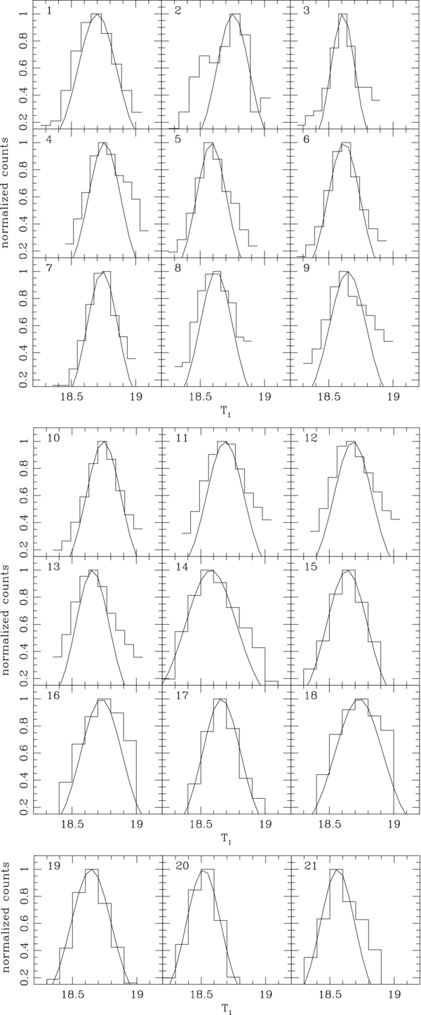
Figure 4. Normalized histograms for the RC T1 mag of the 21 studied LMC fields. The field numbers are labeled at the top left corner of the respective panels. The fitted Gaussians to the RC histograms are also superimposed.
Download figure:
Standard image High-resolution imageTable 4. Mean Reddening Corrected T1o Values (in mag) for the Representative RC Populations in LMC Fields
| Field | A | B | C | D | E | F | G | H | I | J | K | L | M | N | O | P |
|---|---|---|---|---|---|---|---|---|---|---|---|---|---|---|---|---|
| 1 | 18.55 | 18.55 | 18.55 | 18.55 | 18.55 | 18.60 | 18.60 | 18.55 | 18.55 | 18.60 | 18.60 | 18.55 | 18.60 | 18.60 | 18.60 | 18.55 |
| 2 | 18.75 | 18.75 | 18.65 | 18.60 | 18.65 | 18.65 | 18.65 | 18.60 | 18.70 | 18.65 | 18.65 | 18.60 | 18.65 | 18.65 | 18.65 | 18.65 |
| 3 | 18.60 | 18.60 | 18.60 | 18.55 | 18.55 | 18.60 | 18.60 | 18.55 | 18.55 | 18.60 | 18.60 | 18.55 | 18.60 | 18.55 | 18.55 | 18.55 |
| 4 | 18.85 | 18.75 | 18.75 | 18.75 | 18.75 | 18.70 | 18.70 | 18.65 | 18.75 | 18.70 | 18.70 | 18.65 | 18.70 | 18.65 | 18.65 | 18.60 |
| 5 | 18.50 | 18.55 | 18.55 | 18.55 | 18.55 | 18.55 | 18.55 | 18.55 | 18.55 | 18.55 | 18.55 | 18.60 | 18.55 | 18.50 | 18.50 | 18.50 |
| 6 | 18.55 | 18.55 | 18.55 | 18.50 | 18.55 | 18.55 | 18.60 | 18.55 | 18.55 | 18.55 | 18.55 | 18.55 | 18.55 | 18.55 | 18.55 | 18.50 |
| 7 | 18.60 | 18.70 | 18.65 | 18.65 | 18.65 | 18.65 | 18.65 | 18.65 | 18.65 | 18.65 | 18.65 | 18.65 | 18.70 | 18.65 | 18.65 | 18.60 |
| 8 | 18.60 | 18.60 | 18.60 | 18.60 | 18.55 | 18.60 | 18.60 | 18.55 | 18.55 | 18.60 | 18.60 | 18.60 | 18.50 | 18.55 | 18.55 | 18.55 |
| 9 | 18.60 | 18.60 | 18.60 | 18.55 | 18.60 | 18.60 | 18.60 | 18.60 | 18.60 | 18.60 | 18.60 | 18.60 | 18.55 | 18.55 | 18.55 | 18.60 |
| 10 | 18.65 | 18.65 | 18.65 | 18.65 | 18.65 | 18.65 | 18.65 | 18.65 | 18.65 | 18.65 | 18.65 | 18.65 | 18.65 | 18.65 | 18.65 | 18.65 |
| 11 | 18.65 | 18.65 | 18.65 | 18.65 | 18.65 | 18.60 | 18.60 | 18.60 | 18.65 | 18.60 | 18.60 | 18.60 | 18.60 | 18.60 | 18.60 | 18.55 |
| 12 | 18.60 | 18.60 | 18.65 | 18.65 | 18.60 | 18.60 | 18.60 | 18.65 | 18.60 | 18.60 | 18.60 | 18.60 | 18.60 | 18.55 | 18.55 | 18.55 |
| 13 | 18.55 | 18.60 | 18.60 | 18.60 | 18.55 | 18.55 | 18.60 | 18.60 | 18.55 | 18.55 | 18.60 | 18.60 | 18.55 | 18.55 | 18.55 | 18.60 |
| 14 | 18.50 | 18.50 | 18.50 | 18.50 | 18.50 | 18.55 | 18.50 | 18.55 | 18.50 | 18.50 | 18.50 | 18.50 | 18.60 | 18.55 | 18.60 | 18.60 |
| 15 | 18.55 | 18.60 | 18.60 | 18.60 | 18.60 | 18.55 | 18.55 | 18.55 | 18.60 | 18.55 | 18.55 | 18.55 | 18.60 | 18.55 | 18.55 | 18.50 |
| 16 | 18.75 | 18.65 | 18.65 | 18.60 | 18.60 | 18.65 | 18.65 | 18.65 | 18.65 | 18.65 | 18.65 | 18.65 | 18.55 | 18.60 | 18.60 | 18.60 |
| 17 | 18.55 | 18.55 | 18.55 | 18.55 | 18.50 | 18.55 | 18.55 | 18.60 | 18.50 | 18.55 | 18.55 | 18.60 | 18.50 | 18.55 | 18.55 | 18.60 |
| 18 | 18.70 | 18.65 | 18.70 | 18.70 | 18.70 | 18.70 | 18.65 | 18.70 | 18.70 | 18.65 | 18.70 | 18.70 | 18.65 | 18.65 | 18.70 | 18.70 |
| 19 | 18.55 | 18.55 | 18.55 | 18.55 | 18.55 | 18.55 | 18.55 | 18.55 | 18.55 | 18.55 | 18.55 | 18.55 | 18.55 | 18.55 | 18.50 | 18.50 |
| 20 | 18.45 | 18.45 | 18.45 | 18.45 | 18.45 | 18.45 | 18.45 | 18.45 | 18.45 | 18.45 | 18.45 | 18.45 | 18.45 | 18.45 | 18.45 | 18.40 |
| 21 | 18.60 | 18.50 | 18.50 | 18.50 | 18.50 | 18.50 | 18.50 | 18.50 | 18.50 | 18.50 | 18.50 | 18.50 | 18.50 | 18.50 | 18.50 | 18.45 |
Download table as: ASCIITypeset image
4. REPRESENTATIVE LMC FIELD AGES AND METALLICITIES
We are primarily interested in determining the age and metallicity of the representative star population in each field. First, we derived δT1 indices, calculated by determining the difference in the T1 magnitude of the RC and the MS TO (Geisler et al. 1997). The δ(T1) index has proven to be a powerful tool to derive ages for star clusters older than 1 Gyr, independently of their metallicities (Bica et al. 1998; Piatti et al. 2002, 2009, 2011a; Piatti 2011a). Indeed, Geisler et al. (1997) showed that δ(T1) is very well correlated with δ(R) (correlation coefficient = 0.993) and with δ(V). Note that this δT1 measurement technique does not require absolute photometry and is independent of reddening as well. An additional advantage is that we do not need to go deep enough to see the extended MS of the representative star population but only its MS TO. In order to calculate the δT1 values, we used the T1(MSTO) and T1(RC) magnitudes estimated in Sections 3.1 and 3.2, respectively. We then derived ages from the δT1 values using Equation (4) of Geisler et al. (1997). This equation is only calibrated for ages larger than 1 Gyr, so that we are not able to produce ages for younger representative populations. Table 5 presents the resultant ages and their dispersions. These dispersions have been calculated bearing in mind the broadness of the T1 mag distributions of the representative MSTOs and RCs, instead of the photometric errors at T1(MSTO) and T1(RC) mags, respectively. The former are clearly larger, as discussed in Sections 3.1 and 3.2, and represent in general a satisfactory estimate of the age spread around the prevailing population age, although some individual subfields have slightly larger age spreads. These larger age spreads should not affect the subsequent results.
Table 5. Estimated Ages and Dispersions (in Gyr) for the Representative Populations in LMC Fields
| Field | A | B | C | D | E | F | G | H | I | J | K | L | M | N | O | P |
|---|---|---|---|---|---|---|---|---|---|---|---|---|---|---|---|---|
| 1 | 9.0 | 9.0 | 11.7 | 9.0 | 9.0 | 11.1 | 11.1 | 11.7 | 9.0 | 11.1 | 11.1 | 11.7 | 8.6 | 11.1 | 11.1 | 11.7 |
| 2.8 | 2.8 | 3.5 | 2.8 | 2.8 | 3.3 | 3.3 | 3.5 | 2.8 | 3.3 | 3.3 | 3.5 | 2.7 | 3.3 | 3.3 | 3.5 | |
| 2 | 9.5 | 9.5 | 10.5 | 11.1 | 8.1 | 10.5 | 10.5 | 8.6 | 10.0 | 8.1 | 10.5 | 11.1 | 10.5 | 10.5 | 8.1 | 8.1 |
| 2.9 | 2.9 | 3.2 | 3.3 | 2.6 | 3.2 | 3.2 | 2.7 | 3.1 | 2.6 | 3.2 | 3.3 | 3.2 | 3.2 | 2.6 | 2.6 | |
| 3 | 8.6 | 11.1 | 8.6 | 11.7 | 9.0 | 11.1 | 11.1 | 9.0 | 11.7 | 11.1 | 8.6 | 11.7 | 8.6 | 9.0 | 11.7 | 9.0 |
| 2.7 | 3.3 | 2.7 | 3.5 | 2.8 | 3.3 | 3.3 | 2.8 | 3.5 | 3.3 | 2.7 | 3.5 | 2.7 | 2.8 | 3.5 | 2.8 | |
| 4 | 11.1 | 9.5 | 9.5 | 9.5 | 9.5 | 7.7 | 10.0 | 10.5 | 9.5 | 10.0 | 10.0 | 10.5 | 12.9 | 8.1 | 8.1 | 8.6 |
| 3.3 | 2.9 | 2.9 | 2.9 | 2.9 | 2.5 | 3.1 | 3.2 | 2.9 | 3.1 | 3.1 | 3.2 | 3.8 | 2.6 | 2.6 | 2.7 | |
| 5 | 9.5 | 11.7 | 11.7 | 11.7 | 11.7 | 11.7 | 9.0 | 11.7 | 11.7 | 11.7 | 9.0 | 6.5 | 11.7 | 12.3 | 7.3 | 9.5 |
| 2.9 | 3.5 | 3.5 | 3.5 | 3.5 | 3.5 | 2.8 | 3.5 | 3.5 | 3.5 | 2.8 | 2.1 | 3.5 | 3.6 | 2.3 | 2.9 | |
| 6 | 9.0 | 9.0 | 9.0 | 9.5 | 11.7 | 9.0 | 11.1 | 9.0 | 9.0 | 9.0 | 11.7 | 9.0 | 9.0 | 11.7 | 9.0 | 9.5 |
| 2.8 | 2.8 | 2.8 | 2.9 | 3.5 | 2.8 | 3.3 | 2.8 | 2.8 | 2.8 | 3.5 | 2.8 | 2.8 | 3.5 | 2.8 | 2.9 | |
| 7 | 11.1 | 10.0 | 4.7 | 10.5 | 10.5 | 10.5 | 8.1 | 8.1 | 10.5 | 10.5 | 13.5 | 10.5 | 12.9 | 8.1 | 8.1 | 11.1 |
| 3.3 | 3.1 | 1.5 | 3.2 | 3.2 | 3.2 | 2.6 | 2.6 | 3.2 | 3.2 | 3.9 | 3.2 | 3.8 | 2.6 | 2.6 | 3.3 | |
| 8 | 8.6 | 11.1 | 8.6 | 8.6 | 9.0 | 11.1 | 8.6 | 9.0 | 9.0 | 8.6 | 8.6 | 8.6 | 7.3 | 6.9 | 9.0 | 9.0 |
| 2.7 | 3.3 | 2.7 | 2.7 | 2.8 | 3.3 | 2.7 | 2.8 | 2.8 | 2.7 | 2.7 | 2.7 | 2.3 | 2.2 | 2.8 | 2.8 | |
| 9 | 6.5 | 6.5 | 4.9 | 5.2 | 8.6 | 4.9 | 3.7 | 4.9 | 6.5 | 8.6 | 6.5 | 4.9 | 9.0 | 6.9 | 5.2 | 6.5 |
| 2.1 | 2.1 | 1.6 | 1.7 | 2.7 | 1.6 | 1.2 | 1.6 | 2.1 | 2.7 | 2.1 | 1.6 | 2.8 | 2.2 | 1.7 | 2.1 | |
| 10 | 2.7 | 2.1 | 3.5 | 2.7 | 3.5 | 2.1 | 2.1 | 2.1 | 2.1 | 2.1 | 2.7 | 2.1 | 2.7 | 2.7 | 1.7 | 2.1 |
| 0.8 | 0.5 | 1.1 | 0.8 | 1.1 | 0.5 | 0.5 | 0.5 | 0.5 | 0.5 | 0.8 | 0.5 | 0.8 | 0.8 | 0.3 | 0.5 | |
| 11 | 2.7 | 4.7 | 3.5 | 4.7 | 3.5 | 2.8 | 4.9 | 4.9 | 4.7 | 6.5 | 3.7 | 4.9 | 3.7 | 4.9 | 3.7 | 5.2 |
| 0.8 | 1.5 | 1.1 | 1.5 | 1.1 | 0.8 | 1.6 | 1.6 | 1.5 | 2.1 | 1.2 | 1.6 | 1.2 | 1.6 | 1.2 | 1.7 | |
| 12 | 2.8 | 3.7 | 3.5 | 2.7 | 4.9 | 4.9 | 3.7 | 4.7 | 3.7 | 3.7 | 4.9 | 2.8 | 3.7 | 3.9 | 3.9 | 5.2 |
| 0.8 | 1.2 | 1.1 | 0.8 | 1.6 | 1.6 | 1.2 | 1.5 | 1.2 | 1.2 | 1.6 | 0.8 | 1.2 | 1.3 | 1.3 | 1.7 | |
| 13 | 3.0 | 2.8 | 2.8 | 2.8 | 3.0 | 3.9 | 3.7 | 3.7 | 3.9 | 5.2 | 3.7 | 3.7 | 2.3 | 3.9 | 3.0 | 3.7 |
| 0.9 | 0.8 | 0.8 | 0.8 | 0.9 | 1.3 | 1.2 | 1.2 | 1.3 | 1.7 | 1.2 | 1.2 | 0.6 | 1.3 | 0.9 | 1.2 | |
| 14 | 2.0 | 1.6 | 1.6 | 2.0 | 1.5 | 1.4 | 2.0 | 2.3 | 1.6 | 1.5 | 2.4 | 4.2 | 3.7 | 3.2 | 3.7 | 3.7 |
| 0.4 | 0.3 | 0.3 | 0.4 | 0.2 | 0.2 | 0.4 | 0.6 | 0.3 | 0.2 | 0.7 | 1.4 | 1.2 | 1.0 | 1.2 | 1.2 | |
| 15 | 3.9 | 4.9 | 3.7 | 3.7 | 4.9 | 3.9 | 3.9 | 3.9 | 3.7 | 3.9 | 3.9 | 3.2 | 3.7 | 3.2 | 3.0 | 2.4 |
| 1.3 | 1.6 | 1.2 | 1.2 | 1.6 | 1.3 | 1.3 | 1.3 | 1.2 | 1.3 | 1.3 | 1.0 | 1.2 | 1.0 | 0.9 | 0.7 | |
| 16 | 5.5 | 4.7 | 4.7 | 4.9 | 6.5 | 4.7 | 6.2 | 6.2 | 4.7 | 6.2 | 6.2 | 3.5 | 5.2 | 6.5 | 4.9 | 3.7 |
| 1.8 | 1.5 | 1.5 | 1.6 | 2.1 | 2.1 | 2.0 | 2.0 | 1.5 | 2.0 | 2.0 | 1.1 | 1.7 | 2.1 | 1.6 | 1.2 | |
| 17 | 6.9 | 6.9 | 11.7 | 11.7 | 12.3 | 9.5 | 9.5 | 6.5 | 10.0 | 11.7 | 11.7 | 9.0 | 10.0 | 9.5 | 9.5 | 9.0 |
| 2.2 | 2.2 | 3.5 | 3.5 | 3.6 | 2.9 | 2.9 | 2.1 | 3.1 | 3.5 | 3.5 | 2.8 | 3.1 | 2.9 | 2.9 | 2.8 | |
| 18 | 4.4 | 6.2 | 8.1 | 8.1 | 4.4 | 8.1 | 8.6 | 10.0 | 4.4 | 4.7 | 5.8 | 10.0 | 3.5 | 6.2 | 5.8 | 4.4 |
| 1.4 | 2.0 | 2.6 | 2.6 | 1.4 | 2.6 | 2.7 | 3.1 | 1.4 | 1.5 | 1.9 | 3.1 | 1.1 | 2.0 | 1.9 | 1.4 | |
| 19 | 9.5 | 11.7 | 6.9 | 11.7 | 9.0 | 11.7 | 9.0 | 9.0 | 9.0 | 9.0 | 9.0 | 9.0 | 9.0 | 6.9 | 12.3 | 9.5 |
| 2.9 | 3.5 | 2.2 | 3.5 | 2.8 | 3.5 | 2.8 | 2.8 | 2.8 | 2.8 | 2.8 | 2.8 | 2.8 | 2.2 | 3.6 | 2.9 | |
| 20 | 10.0 | 12.9 | 10.0 | 10.0 | 10.0 | 10.0 | 12.9 | 10.0 | 10.0 | 12.9 | 7.7 | 12.9 | 10.0 | 10.0 | 7.7 | 8.1 |
| 3.1 | 3.8 | 3.1 | 3.1 | 3.1 | 3.1 | 3.8 | 3.1 | 3.1 | 3.8 | 2.5 | 3.8 | 3.1 | 3.1 | 2.5 | 2.6 | |
| 21 | 8.6 | 12.3 | 9.5 | 9.5 | 12.3 | 12.3 | 12.3 | 12.3 | 9.5 | 12.3 | 9.5 | 12.3 | 9.5 | 9.5 | 12.3 | 10.0 |
| 2.7 | 3.6 | 2.9 | 2.9 | 3.6 | 3.6 | 3.6 | 3.6 | 2.9 | 3.6 | 2.9 | 3.6 | 2.9 | 2.9 | 3.6 | 3.1 |
Download table as: ASCIITypeset image
Second, mean metallicities for the fields were obtained using the [ ] plane using the SGBs of Geisler & Sarajedini (1999). They demonstrated that the metallicity sensitivity of the SGBs in the Washington system is three times higher than that of the V, I technique (Da Costa & Armandroff 1990) and that, consequently, it is possible to determine metallicities three times more precisely for a given photometric error. However, the SGBs were defined mainly by using globular clusters older than 10 Gyr and, in view of the well-known age–metallicity degeneracy, it is important to examine as closely as possible the effect of applying such a calibration based on very old objects to much younger clusters. Geisler et al. (2003) explored this effect empirically by using well-known metallicities of 11 intermediate-aged clusters (see their Figure 6), as well as by comparing their results to isochrones. They derived an age-correction procedure that we employ here, which provides age-corrected metallicities in good general agreement with spectroscopic values (e.g., Parisi et al. 2010). The SGBs have been profitably used to estimate metallicities with uncertainties ≲0.2 dex for clusters and star fields older than ∼1 Gyr (Piatti et al. 2007, 2011a; Piatti 2011b, 2012, and references therein).
We then followed the standard SGB procedure of entering absolute  magnitudes and intrinsic (C − T1)o colors for each subfield into Figure 4 of Geisler & Sarajedini (1999). The absolute
  magnitudes and intrinsic (C − T1)o colors were obtained from the equations
  = T1 + 0.58E(B − V) − (V − MV) and (C − T1)o = C − T1 − 1.97E(B − V) (Geisler & Sarajedini 1999), where E(B − V) and (V − MV) represent the color excess and the apparent distance modulus. Field reddening values were estimated for each subfield by interpolating the extinction maps of Burstein & Heiles (1982). These maps were obtained from H i (21 cm) emission data for the southern sky and provide us with foreground E(B − V) color excesses which depend on the Galactic coordinates. Subramanian & Subramanian (2009) found that most of the regions have very negligible internal reddening; the regions with the highest internal reddening (E(B − V) = 0.10) are located near the eastern end of the bar and the 30 Dor star-forming region. Table 1 lists the averaged E(B − V) values for the 21 studied LMC fields. As for the LMC distance modulus, we adopted the value (m − M)o = 18.50 ± 0.10 recently reported by Saha et al. (2010). We refer the reader to Bica et al. (1998) and Piatti et al. (2011a), for example, for a detailed analysis about using a unique distance modulus. Then, we entered these (C − T1)o and
  values in Figure 4 of Geisler & Sarajedini as illustrated in Figure 5, which shows the reddening-corrected Hess diagram for the LMC field 19.
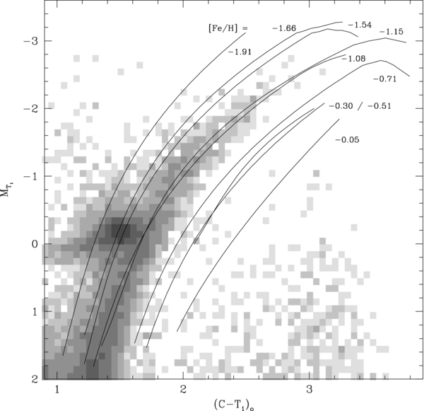
Figure 5. Reddening corrected Hess diagram for the LMC field 19, with standard giant branches from Geisler & Sarajedini (1999) superimposed.
Download figure:
Standard image High-resolution imageWe interpolate the field metal abundance values ([Fe/H]), using the mean position estimated by eye of the whole extension of the RGB, within the isoabundance lines drawn in the figure. Note that the mean position for Fields 9, 16, and 18 is not affected if some amount of differential reddening is present (see also their respective RC profiles in Figure 4). In the case of Figure 5, we measured 〈[Fe/H]〉 = −1.1; the age of the field is (9.0 ± 2.9 Gyr). The metallicities herein derived were then corrected for age effects following the prescriptions given in Geisler et al. (2003), by computing a Δ[Fe/H] value (the metallicity correction) through the expression:
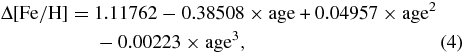
where the units of age and Δ[Fe/H] are Gyr and dex, respectively. Equation (4) is an analytical expression of the solid line traced in Figure 6 by Geisler et al. (2003), which is valid for ages ≳1 Gyr. Note that the correction is negligible for ages >8 Gyr. The Δ[Fe/H] values were subtracted from the measured [Fe/H] to derive the corrected value. In order to take into account the metallicity spread, we assume a dispersion of 0.2 dex for the measured metallicities, although the SGB procedure allows us to estimate [Fe/H] values with an uncertainty of 0.1 dex, to which we added the uncertainties coming from the age corrections in order to assign formal dispersions to the final metallicity values. Table 6 lists the mean metallicity and its dispersion for each studied field. Note that the field RGBs (see Figure 3) are very well populated and show a significant color spread at a given magnitude. It is difficult to tell how much of the observed spread is due to age spread and how much to metallicity spread. Here, we have simply given the mean metal abundance derived from the above analysis.
Table 6. Estimated Metallicities and Dispersions (in dex) for the Representative Populations in LMC Fields
| Field | A | B | C | D | E | F | G | H | I | J | K | L | M | N | O | P |
|---|---|---|---|---|---|---|---|---|---|---|---|---|---|---|---|---|
| 1 | −0.96 | −0.86 | −0.90 | −0.76 | −0.91 | −1.00 | −0.95 | −1.00 | −0.96 | −0.95 | −0.95 | −0.95 | −0.85 | −0.95 | −0.95 | −0.90 |
| 0.31 | 0.31 | 0.20 | 0.31 | 0.31 | 0.20 | 0.20 | 0.20 | 0.31 | 0.20 | 0.20 | 0.20 | 0.28 | 0.20 | 0.20 | 0.20 | |
| 2 | −0.88 | −0.88 | −0.90 | −0.90 | −0.74 | −0.90 | −0.90 | −0.85 | −0.80 | −0.84 | −0.90 | −0.85 | −− | −0.90 | −0.84 | −0.89 |
| 0.35 | 0.35 | 0.20 | 0.20 | 0.26 | 0.20 | 0.20 | 0.28 | 0.20 | 0.26 | 0.20 | 0.20 | 0.20 | 0.20 | 0.26 | 0.26 | |
| 3 | −0.85 | −0.95 | −0.90 | −0.90 | −0.91 | −0.95 | −0.95 | −0.86 | −0.95 | −0.95 | −0.90 | −0.90 | −0.85 | −0.86 | −0.90 | −0.86 |
| 0.28 | 0.20 | 0.28 | 0.20 | 0.31 | 0.20 | 0.20 | 0.31 | 0.20 | 0.20 | 0.28 | 0.20 | 0.28 | 0.31 | 0.20 | 0.31 | |
| 4 | −0.90 | −0.88 | −0.88 | −0.93 | −0.83 | −0.93 | −1.00 | −1.00 | −0.88 | −1.00 | −0.95 | −0.95 | −0.90 | −0.94 | −0.89 | −0.90 |
| 0.20 | 0.35 | 0.35 | 0.35 | 0.35 | 0.25 | 0.20 | 0.20 | 0.35 | 0.20 | 0.20 | 0.20 | 0.20 | 0.26 | 0.26 | 0.28 | |
| 5 | −0.78 | −0.90 | −0.90 | −0.90 | −0.90 | −0.90 | −0.86 | −0.90 | −0.90 | −0.90 | −0.86 | −0.86 | −0.85 | −0.85 | −0.77 | −0.88 |
| 0.35 | 0.20 | 0.20 | 0.20 | 0.20 | 0.20 | 0.31 | 0.20 | 0.20 | 0.20 | 0.31 | 0.25 | 0.20 | 0.20 | 0.24 | 0.35 | |
| 6 | −0.86 | −0.91 | −0.86 | −0.93 | −0.85 | −0.96 | −0.95 | −0.91 | −0.91 | −0.96 | −1.00 | −0.91 | −0.86 | −1.00 | −0.91 | −1.08 |
| 0.31 | 0.31 | 0.31 | 0.35 | 0.20 | 0.31 | 0.20 | 0.31 | 0.31 | 0.31 | 0.20 | 0.31 | 0.31 | 0.20 | 0.31 | 0.35 | |
| 7 | −0.85 | −0.95 | −0.78 | −0.95 | −0.90 | −0.95 | −0.89 | −0.89 | −0.90 | −0.95 | −0.90 | −1.00 | −0.80 | −0.89 | −0.89 | −1.00 |
| 0.20 | 0.20 | 0.31 | 0.20 | 0.20 | 0.20 | 0.26 | 0.26 | 0.20 | 0.20 | 0.20 | 0.20 | 0.20 | 0.26 | 0.26 | 0.20 | |
| 8 | −0.90 | −1.00 | −0.95 | −1.00 | −0.96 | −1.10 | −1.05 | −1.06 | −1.01 | −1.10 | −1.05 | −1.05 | −1.02 | −1.06 | −1.11 | −1.26 |
| 0.28 | 0.20 | 0.28 | 0.28 | 0.31 | 0.20 | 0.28 | 0.31 | 0.31 | 0.28 | 0.28 | 0.28 | 0.24 | 0.24 | 0.31 | 0.31 | |
| 9 | −0.81 | −0.81 | −0.80 | −0.86 | −0.85 | −0.85 | −0.70 | −0.80 | −0.81 | −0.95 | −0.86 | −0.80 | −0.81 | −0.81 | −0.76 | −0.91 |
| 0.25 | 0.25 | 0.30 | 0.29 | 0.28 | 0.30 | 0.33 | 0.30 | 0.25 | 0.28 | 0.25 | 0.30 | 0.31 | 0.24 | 0.29 | 0.25 | |
| 10 | −0.61 | −0.66 | −0.88 | −0.71 | −0.83 | −0.61 | −0.61 | −0.66 | −0.66 | −0.61 | −0.71 | −0.61 | −0.56 | −0.66 | −0.48 | −0.56 |
| 0.33 | 0.31 | 0.34 | 0.33 | 0.34 | 0.34 | 0.31 | 0.31 | 0.31 | 0.31 | 0.33 | 0.31 | 0.33 | 0.33 | 0.28 | 0.31 | |
| 11 | −0.56 | −0.78 | −0.68 | −0.78 | −0.68 | −0.58 | −0.85 | −0.85 | −0.83 | −0.91 | −0.70 | −0.80 | −0.65 | −0.80 | −0.70 | −0.81 |
| 0.33 | 0.31 | 0.34 | 0.31 | 0.34 | 0.34 | 0.30 | 0.30 | 0.31 | 0.25 | 0.33 | 0.30 | 0.33 | 0.30 | 0.33 | 0.29 | |
| 12 | −0.53 | −0.70 | −0.68 | −0.51 | −0.80 | −0.85 | −0.75 | −0.78 | −0.70 | −0.70 | −0.80 | −0.53 | −0.60 | −0.72 | −0.72 | −0.86 |
| 0.34 | 0.33 | 0.34 | 0.33 | 0.30 | 0.30 | 0.33 | 0.31 | 0.33 | 0.33 | 0.30 | 0.34 | 0.33 | 0.33 | 0.33 | 0.29 | |
| 13 | −0.61 | −0.58 | −0.58 | −0.48 | −0.66 | −0.77 | −0.75 | −0.70 | −0.77 | −0.91 | −0.75 | −0.70 | −0.50 | −0.72 | −0.66 | −0.70 |
| 0.34 | 0.34 | 0.34 | 0.34 | 0.34 | 0.33 | 0.33 | 0.33 | 0.33 | 0.29 | 0.33 | 0.33 | 0.32 | 0.33 | 0.34 | 0.33 | |
| 14 | −0.52 | −0.40 | −0.45 | −0.52 | −0.36 | −0.40 | −0.42 | −0.45 | −0.35 | −0.31 | −0.52 | −0.69 | −0.65 | −0.58 | −0.65 | −0.65 |
| 0.30 | 0.27 | 0.27 | 0.30 | 0.26 | 0.25 | 0.30 | 0.32 | 0.27 | 0.26 | 0.33 | 0.32 | 0.33 | 0.34 | 0.33 | 0.33 | |
| 15 | −0.67 | −0.80 | −0.70 | −0.65 | −0.80 | −0.77 | −0.77 | −0.77 | −0.70 | −0.77 | −0.77 | −0.73 | −0.65 | −0.68 | −0.71 | −0.67 |
| 0.33 | 0.30 | 0.33 | 0.33 | 0.30 | 0.33 | 0.33 | 0.33 | 0.33 | 0.33 | 0.33 | 0.34 | 0.33 | 0.34 | 0.34 | 0.33 | |
| 16 | −0.67 | −0.73 | −0.68 | −0.75 | −0.81 | −0.73 | −0.80 | −0.80 | −0.73 | −0.75 | −0.80 | −0.63 | −0.66 | −0.76 | −0.75 | −0.60 |
| 0.28 | 0.31 | 0.31 | 0.30 | 0.25 | 0.31 | 0.26 | 0.26 | 0.31 | 0.26 | 0.26 | 0.34 | 0.29 | 0.25 | 0.30 | 0.33 | |
| 17 | −0.91 | −0.91 | −1.15 | −1.05 | −1.20 | −1.18 | −1.13 | −0.96 | −1.25 | −1.15 | −1.15 | −1.06 | −1.15 | −1.13 | −1.13 | −1.11 |
| 0.24 | 0.24 | 0.20 | 0.20 | 0.20 | 0.35 | 0.35 | 0.25 | 0.20 | 0.20 | 0.20 | 0.31 | 0.20 | 0.35 | 0.35 | 0.31 | |
| 18 | −0.71 | −0.70 | −0.74 | −0.74 | −0.61 | −0.74 | −0.75 | −0.80 | −0.71 | −0.63 | −0.69 | −0.80 | −0.63 | −0.70 | −0.69 | −0.61 |
| 0.31 | 0.26 | 0.26 | 0.26 | 0.31 | 0.26 | 0.28 | 0.20 | 0.31 | 0.31 | 0.27 | 0.20 | 0.34 | 0.26 | 0.27 | 0.31 | |
| 19 | −1.13 | −1.10 | −0.96 | −0.95 | −1.01 | −1.15 | −1.11 | −1.11 | −1.06 | −1.11 | −1.11 | −1.11 | −0.96 | −1.06 | −1.15 | −1.28 |
| 0.35 | 0.20 | 0.24 | 0.20 | 0.31 | 0.20 | 0.31 | 0.31 | 0.31 | 0.31 | 0.31 | 0.31 | 0.31 | 0.24 | 0.20 | 0.35 | |
| 20 | −1.15 | −1.30 | −1.30 | −1.10 | −1.25 | −1.30 | −1.25 | −1.20 | −1.20 | −1.20 | −1.13 | −1.15 | −1.10 | −1.20 | −1.13 | −1.24 |
| 0.20 | 0.20 | 0.20 | 0.20 | 0.20 | 0.20 | 0.20 | 0.20 | 0.20 | 0.20 | 0.25 | 0.20 | 0.20 | 0.20 | 0.25 | 0.26 | |
| 21 | −0.85 | −0.95 | −0.93 | −0.98 | −0.95 | −1.00 | −1.00 | −1.00 | −0.93 | −1.05 | −1.03 | −1.00 | −0.88 | −1.03 | −1.10 | −1.15 |
| 0.28 | 0.20 | 0.35 | 0.35 | 0.20 | 0.20 | 0.20 | 0.20 | 0.35 | 0.20 | 0.35 | 0.20 | 0.35 | 0.35 | 0.20 | 0.20 |
Download table as: ASCIITypeset image
Table 7. C and T1 Magnitudes Reached at a 50% Completeness Level for the 21 Studied LMC Fields
| Field | C | T1 |
|---|---|---|
| 1 | 24.50 | 23.50 |
| 2 | 24.40 | 23.50 |
| 3 | 24.25 | 23.50 |
| 4 | 24.60 | 23.50 |
| 5 | 24.10 | 23.50 |
| 6 | 23.90 | 23.25 |
| 7 | 24.70 | 23.90 |
| 8 | 24.00 | 23.30 |
| 9 | 23.70 | 23.40 |
| 10 | 24.40 | 23.40 |
| 11 | 23.70 | 23.25 |
| 12 | 23.90 | 23.50 |
| 13 | 24.10 | 23.50 |
| 14 | 24.00 | 23.30 |
| 15 | 24.00 | 23.30 |
| 16 | 23.80 | 23.70 |
| 17 | 24.30 | 23.70 |
| 18 | 23.80 | 23.50 |
| 19 | 24.00 | 23.60 |
| 20 | 24.00 | 23.70 |
| 21 | 24.00 | 23.50 |
Download table as: ASCIITypeset image
5. REVISITING THE VS FEATURE
Piatti et al. (Piatti et al. 1999, hereafter P99) identified a striking feature in the RC region in the CMDs of 21 LMC fields observed by them (small boxes in Figure 1). In addition to the normal RC, most of the CMDs also show a VS composed of stars that lie below the RC and extend from the bottom, bluer edge of the RC to ∼0.45 mag fainter. The VS spans the bluest and faintest color range of the RC. The RCs of their 21 LMC fields are nearly located at the same magnitude and color, centered at ∼18.5 and 1.60 mag, respectively. The constancy of the location in the CMD also appears to be the case for the VS, even in those fields where the VS arises as a small and sparse group of stars. Moreover, the VS maintains not only its mean position but also its verticality in fields where the RC is slightly tilted, following approximately the reddening vector. Thus, they defined VS stars as those stars that fall in the rectangle T1 = 18.75–19.15 and C − T1 = 1.45–1.55. This definition results in a compromise between maximizing the number of VS stars and minimizing contamination from, among other sources, MS, RGB, sub-giant branch, and red horizontal branch stars. The continuous nature of this feature is clearly evident in their Figure 4.
P99 showed that there is a strong correlation between the number of VS stars in the field and the number of LMC giants in the same area. For example, the lowest VS star counts occur in the outermost LMC fields, where the number of red giants is also at a minimum. This result demonstrates that VS stars belong to the LMC and that they are not composed of old objects in the LMC or of a background population of RGC stars. P99 also determined that VS stars are only found in those fields that satisfy some particular conditions, such as containing a significant number of 1–2 Gyr old stars and having metallicities higher than [Fe/H] ≈ −0.9 dex, in good agreement with Girardi's (1999) models, which predicted that a minimum in the luminosity of core He burning giants is reached just before degeneracy occurs for objects with these characteristics. These conditions constrain the VS phenomenon to appear only in some isolated parts of the LMC, particularly those with a noticeable large giant population. However, a large number of RG stars of the appropriate age and metallicity is not a sufficient requisite for forming VS stars.
We here take advantage of the present database to extensively revisit the VS phenomenon in the LMC by following the same analysis undertaken by P99 to obtain the aforementioned relationship (see their Figure 5). We assume the existence of such a feature in the CMD and explore whether the number of stars found inside the VS rectangle has any correlation with the number of VS stars found by P99. First of all, we counted the number of stars in each of our 336 subfields (9' × 9') using the VS rectangle defined by P99. In order to ensure counting stars in the VS rectangle as defined by P99, we first corrected our photometry for interstellar absorption with respect to P99's fields, so that our VS regions are placed correctly and centered on P99's Figure 4. We then normalized the VS counts to the same area coverage (P99's field size is 13 5 ×135). We also counted the number of stars in a larger region, defined by P99 from T1 = 17.5 down to 19.7 and from C − T1 = 1.0 up to 2.2 mag. The stars counted in this region are called RC box stars. Figure 6 illustrates, as an example, the RC boxes of the 16 subfields of Field 21. Each panel is labeled with the corresponding subfield identification and includes the VS rectangle used to count the number of stars located inside it. As can be seen, the VS rectangles are not well populated in any of the RC boxes.

Figure 6. RC boxes for the 16 subfields of Field 21. The subfield identification is given at the bottom of each panel. The VS rectangle is also drawn.
Download figure:
Standard image High-resolution imageThe top left panel of Figure 7 depicts the resultant relationship between the number of stars found inside the VS box and the number of RC box stars. The black filled circles reproduce P99's Figure 5, while the dotted line represents an extrapolation for P99's fields where they found a remarkable number of VS stars. The solid line extrapolates from their Figure 5 the relationship for regions where the VS phenomenon is not clearly present. As can be seen, the number of stars in the VS box is, in general, a function of the number of RC box stars, with a non-negligible dispersion. In addition, comparing the trend for VS fields (dotted line) and that for regions without an increased number of VS stars (solid line), we conclude that the VS phenomenon observed by P99 is not seen in most of the presently studied LMC fields.
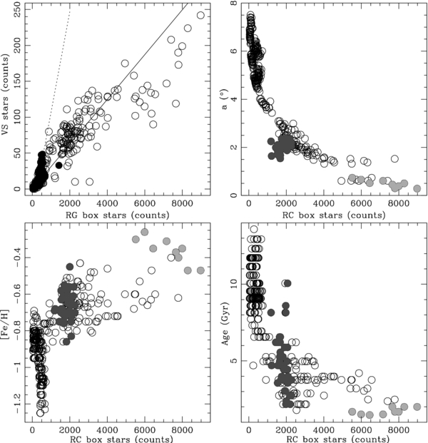
Figure 7. Relationship between the number of VS stars and the number of RG box stars for the studied LMC fields (top left panel), where the black filled circles reproduce Figure 5 of Piatti et al. (1999). The relationships of the RC box stars with the age, the metallicity ([FeH]), and the semimajor axis (a) are also shown. Dark-gray filled circles represent subfields with ∼1700 ± 500 RC box stars distributed throughout a thin ring of size a ∼(2.0 ± 0.5)°, while light gray filled circles correspond to subfields where stellar populations of ≈1–2 Gyr prevail.
Download figure:
Standard image High-resolution image
Figure 8. Schematic figure of the full field and the locations of the subfields labeled within the field.
Download figure:
Standard image High-resolution image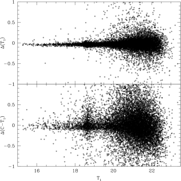
Figure 9. T1 and C − T1 differences for stars observed in both Field 12 and 13. Field 12 resulted to be 0.027 ± 0.111 mag brighter and 0.001 ± 0.332 mag bluer than Field 13.
Download figure:
Standard image High-resolution imageFinally, we investigated some properties of RC box stars taking advantage of their wide observed range. On the one hand, we found that the number of RC box stars decreases—with some exception—as the deprojected distance (a) increases, as is shown in the top right panel of Figure 7. The deprojected distance is here calculated assuming that all the fields are part of a disk having an inclination i = 358 and a position angle of the line of nodes of Θ = 145° (Bica et al. 1998; Olsen & Salyk 2002). Indeed, small numbers of RC box stars (≲1000) are found in the outermost regions (a ≳ 3° in the top right panel), whereas in the innermost regions (a ≲ 1°) they are at least five times more numerous RC box stars. On the other hand, the bottom panels show that smaller numbers of RC box stars (≲1000) span the whole representative age (right panel) and metallicity (left panel) ranges in that part of the galaxy, whereas larger numbers of RC box stars (≳5000) have much younger ages and are more metal-rich.
The top right panel also presents two peculiarities which deserve our attention. One of these peculiar features is a spur-like concentration of stars at RC box stars ∼1700 ± 500 distributed throughout a thin ring of size a ∼(2.0 ± 0.5)°, represented by dark-gray filled circles. This feature embraces the entire Field 16, most of the Field 18, and some parts of the Fields 10 and 13. This relatively constant number of RC box stars is composed by stars with ages between ∼2 and 10 Gyr (see bottom right panel) and metallicities from [Fe/H] ∼ −0.9 up to −0.4 dex (see bottom left panel). The other peculiar feature is that RC box stars distributed in fields where stellar populations of ≈1–2 Gyr prevail are found in the innermost region of the LMC (a < 1°) and within a relatively small [Fe/H] range. We represent these LMC subfields with light gray filled circles. At this age range, we observe an important range of RC box stars (see bottom right panel). However, while these fields are located in the innermost region of the LMC, those of P99 with similar ages and metallicities are placed in the outer disk, where we would have expected to have few RC box stars. Note that according to P99's results, a large proportion of 1–2 Gyr old stars mixed with older stars and with metallicities higher than [Fe/H] ≈ −0.7 dex should result in a clear VS, although they suggested that in order to trigger the formation of VS stars, there should be other conditions in addition to the appropriate age, metallicity, and the necessary red giant star density. Note that all of P99's fields lie relatively near to each other, in a distant northern part of the LMC, and have no overlap with any of our fields studied here (Figure 1). It may be that whatever other parameter plays a role in triggering the VS phenomenon is limited to a particular region of the LMC.
6. SUMMARY
In this study we present, for the first time, CCD Washington CT1T2 photometry of some 5.5 million stars in twenty-one 36' × 36' fields distributed throughout the entire LMC main body. The analysis of the photometric data—subdivided in 336 smaller 9' × 9' fields—leads to the following main conclusions.
- 1.After extensive artificial star tests over the whole mosaic image data set, we show that the 50% completeness level is reached at C ∼ 23.5–25.0 and T1 ∼ 23.0–24.5, depending on the crowding and exposure time, and that the behavior of the photometric errors with magnitude for the observed stars guarantees the accuracy of the morphology and position of the main features in the CMDs that we investigate.
- 2.We obtained T1(MSTO) magnitudes for the so-called representative stellar population of each field, namely, the TO with the largest number of stars. The resultant representative T1(MSTO) mags are on average ∼0.5 mag brighter than the T1 mags for the faintest 100% completeness level of the respective field, so that we reach the TO of the representative population of each field with negligible loss of stars. The prevailing TOs are typically ∼25%–50% more frequent than the following less dominant population, represented by a secondary peak—sometimes there also exists a third peak—in the differential LFs.
- 3.We also investigated the RCs of the studied LMC fields, assuming that the peak of T1(RC) mag distribution corresponds to the most populous T1(MSTO) in the respective field. We built T1 histograms for these RC stars and performed Gaussian fits to derive the mean RC mag values and the FWHMs of the T1(RC) distributions.
- 4.δT1 indices, calculated by determining the difference in the T1 magnitude of the RC and the MSTO, were computed using the representative T1(MSTO) and T1(RC) mags. From these values we estimated the ages of the prevailing population in the studied LMC field, using a well-proven δT1 index–age calibration. The dispersions associated with the mean values represent in general a satisfactory estimate of the age spread around the prevailing population ages, although a few individual subfields have slightly larger age spreads. These larger age spreads do not affect the subsequent results. We also estimated representative metallicities following the standard SGB procedure of entering absolute
 magnitudes and intrinsic (C − T1)o colors for each subfield into Figure 4 of Geisler & Sarajedini (1999). The measured metallicity values were corrected by applying a robust procedure which takes into account the age–metallicity degeneracy effect.
 - 5.Finally, we revisited the study of the VS phenomenon—a striking feature composed of stars that lie below the RC and extend from the lower blue end of the RC to ∼0.45 mag fainter—taking advantage of the present database. We confirm that the VS phenomenon is not clearly seen in most of the studied fields and suggest that its occurrence is linked to some other condition(s) in addition to the appropriate age, metallicity, and the necessary red giant star density.

We greatly appreciate the comments and suggestions raised by the reviewer which helped us to improve the manuscript. We are gratefully indebted to the CTIO staff for their hospitality and support during the observing run. This work was partially supported by the Argentinian institutions CONICET and Agencia Nacional de Promoción Científica y Tecnológica (ANPCyT). D.G. gratefully acknowledges support from the Chilean BASAL Centro de Excelencia en Astrofísica y Tecnologías Afines (CATA) grant PFB-06/2007. We acknowledge contributions from C. Parisi, S. Villanova, J. Holtzman, A. Sarajedini, and L. Girardi.
APPENDIX A: MOSAIC II's FIELD
In order to deal with comparable-sized individual areas to Harris & Zaritsky (2009) and Rubele et al. (2012), we subdivided each 36' ×36' field into 16 uniform 2 K×2 K regions (9' ×9'), and labelled such subfields with letters A to P moving from the west to the east and from the south to the north, as it can be seen in Figure 8.
APPENDIX B: COMPLETENESS OF THE PHOTOMETRIC DATABASE AND EXTERNAL PHOTOMETRIC ERRORS
Although we analyzed data for each field to the magnitude where the completeness level begins to fall below 100%, we include here for completeness purposes Table 7, which lists the mean values of the C and T1 magnitudes reached at a 50% completeness level for the 21 studied LMC fields. Finally, Figure 9 shows the comparison between the photometry for stars measured in Fields #12 and 13. As can be seen, Field #12 resulted to be 0.027 ± 0.111 mag brighter and 0.001 ± 0.332 mag bluer than Field #13.
Footnotes
- 3
IRAF is distributed by the National Optical Astronomy Observatory, which is operated by the Association of Universities for Research in Astronomy, Inc., under cooperative agreement with the National Science Foundation.