


ABSTRACT
Using wide-field J, H, and Ks images obtained with the WIRCam near-infrared camera on the Canada–France–Hawaii Telescope, we investigated the spatial density configuration of stars within the tidal radius of metal-poor globular cluster NGC 6626, which is known to be located near the bulge region and have a thick-disk orbit motion. In order to trace the stellar density around a target cluster, we sorted the cluster's member stars using a mask-filtering algorithm and weighted the stars on the color–magnitude diagram. From the weight-summed surface density map, we found that the spatial density distribution of stars within the tidal radius is asymmetric with distorted overdensity features. The extending overdensity features are likely associated with the effects of the dynamic interaction with the Galaxy and the cluster's space motion. An interesting finding is that the prominent overdensity features extend toward the direction of the Galactic plane. This orientation of stellar density distribution can be interpreted with the result of the disk-shock effect of the Galaxy, previously experienced by the cluster. Indeed, the radial surface density profile accurately describes this overdensity feature with a break in the slope inside the tidal radius. Thus, the observed results indicate that NGC 6626 experienced a strong dynamical interaction with the Galaxy. Based on the result of strong tidal interaction with the Galaxy and previously published results, we discussed possible origins and evolutions of the cluster: (1) the cluster might have formed in satellite galaxies that were merged and created the Galactic bulge region in the early universe, after which time its dynamical properties were modified by dynamical friction, or (2) the cluster might have formed in primordial and rotationally supported massive clumps in the thick disk of the Galaxy.
Export citation and abstract BibTeX RIS
1. INTRODUCTION
In modern cold dark matter cosmology, early galaxy structures are developed hierarchically through a process of progressive merging or accretion events involving small substructures (Baugh et al. 1996; Klypin et al. 1999; Moore et al. 1999). These merging progressions predict that the halo of galaxies, such as the Milky Way, form through the tidal disruption and accretion of numerous low-mass fragments, such as satellite galaxies (Johnston 1998; Bullock et al. 2001; Abadi et al. 2006; Font et al. 2006; Moore et al. 2006). As a result, galaxy halos contain merger relics in the form of long stellar streams and tails that survived for several Gyrs (Bullock & Johnston 2005). Thus, such tidal structures like stellar streams and tails play a key role in providing both direct observational evidence to support the accretion scenario of the Milky Way formation and information regarding their progenitor. Furthermore, the morphological shape of the tidal structure and alignment of streams with the orbit of the progenitor provide an opportunity to reconstruct the orbit of the progenitor (Binney 2008; Eyre & Binney 2009) and study the potential of the Milky Way (Odenkirchen et al. 2009) as well as the ongoing dissolution process.
Recently, with the assistance of wide-field detectors and survey projects, several stellar streams, which disrupted from satellite galaxies in the outer halo of the Milky Way, have been discovered (Helmi et al. 1999; Ivezić et al. 2000; Yanny et al. 2000, 2003; Newberg et al. 2002, 2009; Martin et al. 2004; Rocha-Pinto et al. 2004; Martinez-Delgado et al. 2005; Duffau et al. 2006; Grillmair 2006; Jurić et al. 2008). Along with the most striking example, namely, the Sagittarius dwarf galaxy and its stellar streams (Ibata et al. 1994, 1995, 1997, 2001; Vivas et al. 2001; Majewski et al. 2003; Newberg et al. 2003; Martinez-Delgado et al. 2004; Belokurov et al. 2006b), the tidal streams associated with newly discovered faint dwarf galaxies, or stellar substructures, the parent galaxies of which are unknown (Klement et al. 2009), are now being gradually found. Such examples include the Bootes III dSph (Carlin et al. 2009; Grillmair 2009) and Orphan Stream (Grillmair 2006; Zucker et al. 2006; Belokurov et al. 2007). These broad extended stellar streams in the outer halo of the Milky Way imply that the outer Galactic halo forms via accretion and merging events, and that most of the stellar population in the halo originated from more complex systems (Lynden-Bell & Lynden-Bell 1995).
Some of these stellar streams and substructures might form in or be associated with the globular clusters disrupted by the tidal force of the Milky Way. In recent studies, it has been revealed that most globular clusters contain two or more stellar populations, and some globular clusters are even considered the surviving remnants of much more massive populations that merged into the Milky Way. Since several dwarf spheroidals of the Milky Way such as the Sagittarius (Bellazzini et al. 2003; Tautvaišienė et al. 2004; Sbordone et al. 2005) and Fornax (Buonanno et al. 1998, 1999) dwarf galaxies have their own globular clusters, these globular clusters could fall into the Milky Way and contribute the clusters in the halo of Milky Way in the accretion process. Indeed, Lee et al. (1999) detected multiple stellar populations with different ages and metallicities in ω Centauri, and subsequently confirmed that this most massive object might be the nucleus of a dwarf galaxy that merged into the Milky Way. Several studies further increased the possibility that this hypothesis is correct by detecting multiple stellar populations for many globular clusters (Ferraro et al. 2009; Han et al. 2009; Lee et al. 2009). Mackey & Gilmore (2004) suggested that 41 (27%) of the Milky Way's globular clusters were accreted. Thus, if globular clusters formed via accretion or merging of more complex systems, the globular clusters would be surrounded by stellar substructures that were distorted from the clusters and/or from their parent galaxies. Indeed, well-developed tidal tails and streams are found around Palomar 5 (Odenkirchen et al. 2001; Grillmair & Dionatos 2006a) and NGC 5466 (Belokurov et al. 2006a; Grillmair & Johnson 2006), and slightly extended tidal structures are detected around many globular clusters (Grillmair et al. 1995; Leon et al. 2000; Sohn et al. 2003). Spatially narrow tidal streams such as the GD-1 stream (Grillmair & Dionatos 2006b) and the Acheron, Cocytos, and Lethe streams (Grillmair 2009) are also considered the definite remnants of disrupted globular clusters. Thus, we could find more stellar streams that would be associated with globular clusters in the halo of the Milky Way; from these substructures, we can find constraints on the accretion and merging scenario of galaxy formation. Recently, Chun et al. (2010) found additional extratidal tails around five metal-poor halo globular clusters and added further observational evidence of a merging scenario in the formation of the Galactic halo.
Nevertheless, such studies have focused primarily on the Galactic halo region because of the high value of extinction and contamination of field stars in the bulge region. However, the study of stellar substructures for globular clusters in the Galactic bulge region would also be valuable in terms of understanding the formation of the Galactic bulge. In a hierarchical model, the bulge of a spiral galaxy like the Milky Way formed through a short series of starbursts triggered by the merging of multiple subclumps in a protogalactic cloud (Katz 1992; Baugh et al. 1996; Zoccali et al. 2006). Particularly, Nakasato & Nomoto (2003) suggested that the merging of a subclump in an early universe could cause the metallicity of the stars within the bulge to become as wide as −1.5 ⩽ [Fe/H] < 0.5 (McWilliam & Rich 1994; Zoccali et al. 2003), as this was observed in the Milky Way bulge region. In this sense, many remnants of the first building blocks could remain in the Galactic bulge region. Indeed, Ferraro et al. (2009) found that bulge globular cluster Terzan 5 has two discrete stellar populations with both different metallicities and age, suggesting that it is a surviving remnant of the first building blocks. Therefore, we could discover extratidal substructures around some of the globular clusters in the bulge region from which we anticipate obtaining the constraints on the formation and evolution of the Galactic bulge.
In this study, we investigated the spatial density distribution of stars around NGC 6626 (M28). NGC 6626 is a metal-poor globular cluster of [Fe/H] = −1.32 (Harris 1996) in the Galactic bulge region, i.e., at a distance of ∼2.7 kpc from the Galactic center (Noyola & Gebhardt 2006). Here, we assigned the bulge region as the area within 3 kpc from the Galactic center. It is also known to have extended horizontal branch (EHB) stars (Lee et al. 2007) and a thick-disk-like orbit motion (Cudworth & Hanson 1993). Based on the characteristics of the EHB globular cluster and its peculiar kinematics (low total energy Etot), Lee et al. (2007) suggested that NGC 6626 could be a remnant of the first building block that assembled and initially formed the bulge region in the early universe. Table 1 shows the basic parameters of NGC 6626. In order to reduce the effect of high extinction toward the bulge and adjust our scientific objective, we used wide-field (21' × 21') near-infrared JHKs photometric data obtained from the observation of the WIRCam detector attached to the Canada–France–Hawaii Telescope (CFHT). Section 2 presents the observation, data reduction process, and photometric measurements. The statistical analysis and filtering technique for member star selection are described in Section 3. In Section 4, we investigate two-dimensional stellar density maps and the radial profile of the cluster in order to trace the stellar density features. The discussion and conclusion of our investigation are presented in Section 5.
Table 1. Basic Parameters of NGC 6626
| Parameter | Value | Referencea |
|---|---|---|
| α, δ (J2000) (deg) | 276.13, −24.87 | NG06 |
| RGC (kpc) | 2.7 | NG06 |
| rc (arcmin) | 0.24 | TRA95 |
| rt (arcmin) | 11.27 | TRA95 |
| μαcos δ, μδ (mas yr−1) | 0.3 ± 0.50, −3.40 ± 0.90 | CUD93 |
| [Fe/H] | −1.32 | HAR96 |
Notes. RGC indicates distances from the Galactic center. rc and rt are the core radius and tidal radius of a cluster, respectively. aNG06: Noyola & Gebhardt 2006; TRA95: Trager et al. 1995; CUD93: Cudworth & Hanson 1993; HAR: Harris 1996.
Download table as: ASCIITypeset image
2. OBSERVATION AND DATA REDUCTION
Images of NGC 6626 were secured in Queued Service Observing (QSO) of the 3.6 m CFHT on the nights of 2007 July 16–17. The WIRCam detector is the latest wide-field near-infrared mosaic detector of four 2048 × 2048 HgCdTe arrays, which together cover an area of 21' × 21' with a pixel scale of 0 3. Object data were recorded in short (5 s for JHKs) and long (30 s for J, 15 s for H, and 25 s for Ks) exposures to optimize the photometry of bright and faint stars. Five-point dithering with 1' offset was applied in order to reject bad pixels and cosmic rays, as well as to fill in the 45'' gaps between the arrays. To obtain well-sampled stars, each dithered position involved collecting four micro-dithered observations with a small offset of 0.5 pixels. Here, we note that an additional comparison field area outside of the tidal radius of the cluster was observed using the same observation strategy as the target cluster. This comparison field will be used to estimate the field star contamination (see Section 3). The observation summary is shown in Table 2.
Table 2. Observation Log for NGC 6626 and a Comparison Field
| Target | Filter | Exp. Time | FWHM |
|---|---|---|---|
| (s) | ('') | ||
| NGC 6626 | J | 4 × 5 × 5, 4 × 5 × 30 | 0.73, 0.72 |
| H | 4 × 5 × 5, 4 × 5 × 15 | 0.72, 0.68 | |
| Ks | 4 × 5 × 5, 4 × 5 × 25 | 0.69, 0.67 | |
| comparison | J | 4 × 5 × 5, 4 × 5 × 30 | 0.72, 0.67 |
| H | 4 × 5 × 5, 4 × 5 × 15 | 0.72, 0.76 | |
| Ks | 4 × 5 × 5, 4 × 5 × 25 | 0.66, 0.69 |
Download table as: ASCIITypeset image
The initial process of data reduction was performed with the IDL Interpretor of the WIRCam Images (I'IWI) pipeline at CFHT, which includes dark subtraction, flat fielding, and removal of crosstalk. To continue the processing, thermal emission artifacts were constructed by median-combining the images of blank sky regions, which were recorded after observing the target image; the resulting sky images were then subtracted from all target images. The residual sky background constant level, which was estimated by mode of pixel intensity distribution, was also removed.
Before combining all processed target images, a precise global astrometric solution is required because of a field distortion of about 1% in the corner of the mosaic. A global astrometric solution was derived in comparison with a Two Micron All Sky Survey (2MASS) reference catalog using SCAMP (Bertin 2006), one of the TERAPIX software tools. SCAMP provides a two-dimensional third-order polynomial model of WIRCam image distortions by minimizing a weighted, quadratic sum of differences in position between both overlapping and matched sources of the 2MASS reference catalog. As a result, a reliable and robust astrometric solution with ∼01 rms was derived.
Photometric flux scaling between four arrays is also an important requirement because of the different detector sensitivities, primarily when mosaic images are resampled into one image. The photometric zero points for each detector were computed from standard star observations during WIRCam runs and served in each FITS extension header. SCAMP can derive the photometric solution to scale and normalize the flux of detectors into an arbitrary photometric zero level using these zero-point values. Thus, we again used SCAMP in order to scale and normalize the photometric flux of the four detectors.
All processed images were aligned and interleaved into one image with derived astrometric and photometric solutions. The Swarp (Bertin et al. 2002) task was used to resample and interleave together FITS images. We were then able to obtain a homogeneous wide-field image of 21' × 21', and this provided a sufficiently large area to cover from the center to the tidal radius of NGC 6626. The average seeing condition in resampled images is between 065 and 075; the mean values for short and long exposures are summarized in Table 2.
The photometric measurements of the point sources were measured using the point-spread function fitting routine DAOPHOT II/ALLSTAR (Stetson 1987; Stetson & Harris 1988). Because of the saturation level in long exposures, the brightness of stars around the red giant branch (RGB) tip was measured only in short-exposure images. Nevertheless, since the shortest possible exposure time of the WIRCam was 5 s, stars around the RGB tip were still saturated. On the other hand, only long-exposure images detected faint stars. Measurements with smaller photometric errors were assigned to the brightness for stars detected in both short- and a long-exposure time. Objects in which the measurement error exceeded 0.3 mag were excluded. In order to eliminate spurious detections, we also rejected the stars with χ > 4.0 and |SHARP| > 1.5 values; thus, we were able to remove the objects near the faint limit of the data and extended objects such as faint galaxies. Using the derived astrometric solution and the 2MASS catalog, the instrumental position of the stars was transformed into the equatorial coordinate system, and instrumental magnitudes were calibrated into 2MASS scale. Finally, in order to reduce the effect of interstellar extinction, we derived the individual extinction magnitude for each detected star from the maps of Schlegel et al. (1998). The mean value of E(B − V) from the Schlegel et al. (1998) map is ∼0.47, from which we could derive E(J − K) = 0.22 and Ak = 0.165; these values were then subtracted from the calibrated magnitude.
Figure 1 shows a (J − Ks, Ks)0 dereddened color–magnitude diagram (CMD) of the resolved stars in the region 3 5 from the cluster center. By doing artificial star experiments, we also attached the completeness fraction in the Ks magnitude on the right side of the CMD in order to show uncertainties in the photometric measurements. To clarify the cluster locus on the CMD, we overplotted the Yonsei-Yale (Y2) isochrone (Kim et al. 2002; Yi et al. 2003) of the cluster with a line. The metallicity and age of the cluster were adopted as [Fe/H] = −1.32 (Harris 1996) and 13 Gyr, respectively. The adopted absolute distance modulus was (m − M)0 = 13.64 (Testa et al. 2001), which was calculated from the apparent distance modulus of (m − M)V = 14.97 and the reddening value of E(B − V) = 0.4 (Harris 1996). The isochrone was transformed to the 2MASS system from the ESO system using the transformation equation given by Carpenter (2001). It is apparent that there are a significant number of field star contaminations around the cluster sample. The bulk of the field stars on the right side of the RGB of the cluster are metal-rich bulge RGB stars. The bulge main sequence also shows a tendency of being broad with an increase in magnitude due to photometric errors. The disk main-sequence stars dispersed along the line of sight are also present at some level: a vertical sequence extending upward and blueward from Ks ∼ 16.0 and (J − Ks) ∼ 0.35.

Figure 1. Left panel: (Ks, J − Ks)0 dereddened CMD of NGC 6626 for the stars in the central 35 from the cluster center. The Y2-isochrone line with a metallicity of [Fe/H] = −1.32 and age of 13 Gyr is overplotted with a line. The absolute distance modulus of (m − M)0 = 13.64 is adopted. Right panel: completeness fraction in Ks magnitude obtained from artificial star experiments. The stars brighter than Ks = 18.5 with a completeness of ∼70% are used in the following analysis.
Download figure:
Standard image High-resolution image3. PHOTOMETRIC FILTERING FOR MEMBER STAR SELECTION
The region around the bulge cluster is a location where stars released from the cluster and from the bulge or the disk mix. Consequently, a method is needed to minimize the contaminating field stars and enhance the contrast between the cluster and field stars in order to trace an accurate spatial distribution of the cluster stars. In terms of solving this problem, Grillmair et al. (1995) developed the color–magnitude (hereafter C–M) mask filtering technique, which works by finding the region on the CMD where the signal-to-noise ratio (S/N) of cluster star counts is maximized in contrast to comparison field stars. Odenkirchen et al. (2001) also introduced an advanced method to compress the photometric data in a C–M space in order to compensate for poor statistics, which occurs when the C–M mask filtering technique is applied to sparsely populated globular clusters (see also Chun et al. 2010). In order to enhance the contrast between cluster stars and field stars, in the following description we employed the C–M mask filtering technique used by Odenkirchen et al. (2001) and give additional weight value to the C–M plane.
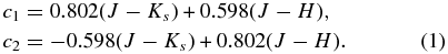
We first defined the new orthogonal color indices c1 and c2 in the (J − Ks) versus (J − H) color–color diagram. Figure 2 shows the (J − Ks) versus (J − H) color–color diagram of stars in the central region, located within half-mass radius (∼ rh). The one-dimensional distribution of NGC 6626 stars was described by solid line with a slope of α = 0.745. The color index c1 axis was chosen to lie along the main axis of the almost one-dimensional distribution of NGC 6626 stars, while the perpendicular axis to c1 axis was assigned as a c2 axis (e.g., Odenkirchen et al. 2001, 2003). Equation (1) presents the newly derived color indices c1 and c2.
Here, for the most part, the systematic variation of color with magnitude is contained in c1, while variations in c2 are due to the observational photometric errors, as noted in Odenkirchen et al. (2001).
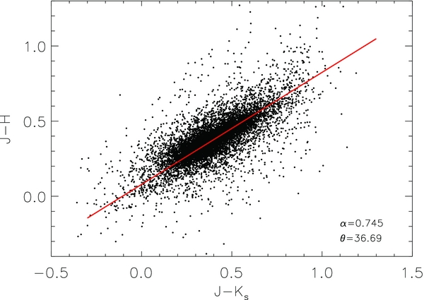
Figure 2. (J − Ks) and (J − H) color–color diagram. Stars in the half-mass radius (∼rh) were used. The line is the fitted line to the main axis of the one-dimensional distribution of NGC 6626 stars. The slope of the fitted line is α = 0.745 from which we could derive an angle of the fitted line of θ = 36.69. This angle was used to define new orthogonal color indices c1 and c2.
Download figure:
Standard image High-resolution imageIn (c2, Ks) space, the sample was preselected by discarding all stars with  , where
  are the photometric errors in c2 for stars with a magnitude of Ks. In order to reduce the crowding effect and field star contamination, the stars within an annulus between 2rc and 10rc from the cluster center were used to derive our discarding limit. The leftmost panel in Figure 3 shows a (c2, Ks) CMD of stars within an annulus between 2rc and 10rc from the cluster center. The thick lines are our discarding limit lines, with a magnitude Ks, i.e.,
  limits.

Figure 3. (c2, Ks) and (c1, Ks) color–magnitude diagram (CMD) of stars in the field of NGC 6626. The leftmost panel shows the (c2, Ks) CMD of stars within an annulus between 2rc and 10rc in radius from the cluster center. The lines in the (c2, Ks) plane are the  boundary at Ks magnitudes due to a photometric error. The left middle to rightmost panels are the (c1, Ks) CMDs for the stars in the cluster central region, in the assigned comparison region, and in the total field of NGC 6626. The overplotted grid lines in the (c1, Ks) CMDs indicate the region where the signal-to-noise ratios of cluster star counts are maximized through a C–M mask filtering technique. The stars outside the grid lines are highly unlikely to be cluster members.
Download figure:
Standard image High-resolution imageAfter this preselection in the (c2, Ks) plane, the C–M mask filtering technique was applied to the stars in the cluster center as well as to those in the comparison field. To obtain reliable count rates and a truly representative sample in the C–M plane, we determined a central region of the cluster and a comparison region. The cluster's central area was assigned so as to have the largest number ratio of stars enclosed  to those outside
  in the (c1, Ks) plane for all preselected stars within the radius of the circle. Here,
  is an estimated standard deviation of c1 for stars with Ks magnitude. The assigned representative of the comparison field is nine times as large an area as the determined central region of the cluster. The (c1, Ks) CMDs of stars in the determined central region of the cluster and the comparison region are shown in the second and third panels from the left in Figure 3, respectively. The rightmost panel shows the (c1, Ks) CMD of the stars in the total survey region for the cluster.
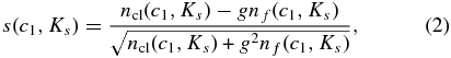
Comparing the (c1, Ks) CMDs of the stars in the selective cluster central region and the comparison region, we then defined the locus of cluster on the (c1, Ks) plane where the stars are highly likely to be cluster members. The C–M plane was subdivided into small subgrid elements with a 0.05 mag width in c1 and a 0.15 mag height in Ks. For each subgrid element, the number of stars for cluster area ncl(c1, Ks) and the number of stars for comparison region nf(c1, Ks) were counted. Assuming that the distribution of background stars on the C–M plane is relatively even across the observed field, the local S/N s(c1, Ks) in each subgrid element for the number of cluster stars was then calculated using basic Poisson statistics of number counts with background subtraction, Equation (2):
where g is the ratio of the cluster region area to that of the comparison region.
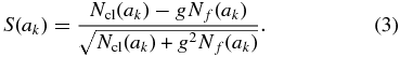
From array s, an optimal mask envelope with a relatively high value of s in the (c1, Ks) plane was obtained by setting a threshold slim < smax (maximum of s) and identifying the subgrid elements of s ⩾ slim. In order to estimate the optimal threshold, we sorted the elements of s(c1, Ks) into a series of descending order with the one-dimensional index of k. Then, a cumulative number of stars in the cluster area Ncl(ak) = ∑kl = 1ncl(l) was counted with the progressively larger area ak = kal, where al is the area of a single element of the C–M plane. We also counted the cumulative star counts for the comparison region Nf(ak) = ∑kl = 1nf(l) in the same manner as for the cluster area. Equation (3) provides the formula for the calculation of the cumulative S/N S(ak):
S(ak) reaches a maximum value for a particular subarea of the C–M plane; therefore, we can set up the value of s(c1, Ks), corresponding to the maximum value of S(ak), as an optimal threshold slim. The filtering mask area in the (c1, Ks) plane was then determined by selecting subgrid elements with larger s(c1, Ks) values than the determined slim. Solid lines in the second, third, and fourth panels, starting from the left in Figure 3, represent the selected optimal mask envelope. The limiting magnitude Ks of the filtering mask area was assigned to be equal to 18.5 with completeness of ∼70% to avoid biases caused by the poor completeness of the photometry (see Figure 1). The entire sample of stars in the determined filtering mask area was considered in the following filtering analysis.
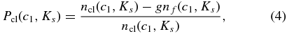
While we have determined the optimal mask envelope with a high-S/N ratio of the cluster to reduce background/foreground field contribution, as shown in Figure 3, there are still a significant number of field stars (i.e., disk and bulge stars) in the determined envelope. Thus, if we merely count the stars in the determined envelope without considering the density of the background field stars in the C–M plane, we could give the same weight to cluster member stars and background field stars, and in the end, reduce the contrast between the cluster stars and the field stars. When we consider the entire sample of stars in the determined mask area, this is especially true and even more serious in the case of our target cluster, NGC 6626, because it has many bulge field stars as shown in the CMD of Figure 1. Therefore, in order to solve this problem, we discriminated the weight of the stars in the determined mask envelope according to the position in the C–M plane. The weight values of the stars in the mask envelope were calculated on the same subgrid map employed in the C–M mask filtering technique, using the stars in the determined cluster central region and comparison region. Equation (4) indicates the weight values at each subgrid element in the (c1, Ks) CMD:
where g, ncl(c1, Ks), and nf(c1, Ks) have the same meaning as in Equation (2). Thus, Pcl(c1, Ks) will have a value ∼1 for regions of the C–M plane in which the cluster sample is not substantially contaminated by field stars or conversely, will decrease and become ∼0, when the field star contamination becomes severe. Pcl(j) functions like the probability of a cluster member. The value of Pcl(c1, Ks) could be less than 0 in some regions in which the number of field stars (gnf) is larger than that of cluster (ncl), and then the probability could break down for such regions. Thus, for these areas, we replaced the values of Pcl(c1, Ks) less than 0 with 0. However, we note that there were no regions with Pcl(c1, Ks) less than 0 in the determined mask envelope because we already assigned the regions with high S/N using the mask filtering technique. Figure 4 shows the distribution of the weight value Pcl(c1, Ks) of cluster membership in the determined optimal envelope of the C–M plane. We overplot the Y2-isochrone of Figure 1 with a solid line. It is clearly visible that most loci of the cluster in the C–M plane have a high value of weight Pcl(c1, Ks). The high-density contour of the faint locus below Ks = 16.5 does not seem to show a good match with the Y2-isochrone. However, the area on the right side of the Y2-isochrone (bluer area than c1 ∼ 0.5) was contaminated by metal-rich bulge field stars, thus the value of Pcl(c1, Ks) is inevitably low, causing left-skewed density contours. These values were used to construct the stellar density distribution map and are subsequently considered in further analysis to examine the spatial configuration around the cluster.

Figure 4. Weights of cluster membership as a function of color and magnitude in the determined optimal envelope. The contour levels are 0.1, 0.3, 0.5, and 0.7 of Pcl. The Y2-isochrone in Figure 1 was transformed into the c1 index and overplotted with a line.
Download figure:
Standard image High-resolution image4. SURFACE DENSITY DISTRIBUTION OF STARS AROUND NGC 6626
4.1. Two-dimensional Stellar Density Distribution
Using stars selected from the statistical process in Section 3, we constructed a two-dimensional stellar surface density map of the cluster from a grid with pixels of 0258 × 0258 in the plane of the sky. The weighted number density was calculated by summing the given weight values Pcl(c1, Ks) of all stars in a grid on the sky. We then smoothed this weighted number density map with a Gaussian smoothing algorithm to enhance the low spatial frequency of the background variation and remove the high frequency of the spatial stellar density variation. The background density map was also constructed from the comparison field. We distributed the same weight values of Pcl(c1, Ks) to the comparison field stars in the masking envelope of Figure 3, and then the weighted number density background map was calculated in the same manner as the cluster density map. The mean background level and standard deviation were both estimated from the resulting background density map.
The top panel in Figure 5 is the resulting weighted star count map of stars, and the second and third panels are its isodensity contour plots smoothed with kernel values of ∼10 and ∼22, respectively. The isodensity contour lines are drawn at the levels of σ, 2σ, 2.5σ, 3σ, 3.5σ, 4σ, 4.2σ, and 5σ above the background density level. σ is the standard deviation obtained from the background density map. The two white boxes on the east corners represent the detector area at which the WIRCam array has intrinsic deficiencies. The data in these areas were excluded from the density map and subsequent analysis because of a poor number of stars. The contours in the weighted star count map are the same as those in the contour map smoothed with a Gaussian kernel value of 22. We also indicated the direction toward the Galactic center (solid line) and the perpendicular direction to the Galactic plane (dashed line). The direction of Galactic motion of the cluster, based on the proper motion with μαcos δ = 0.30 ± 0.50 mas yr−1 and μδ = −3.40 ± 0.90 mas yr−1 (Cudworth & Hanson 1993), is represented by a solid arrow. The large circle indicates a tidal radius of rt = 1127 (Trager et al. 1995). Chen & Chen (2010) examined the shapes and sizes of several globular clusters using the 2MASS point sources. They found that many globular clusters near the Galactic bulge region exhibit obvious flattening in shape, and described the elongation of clusters with morphological parameters such as the semimajor/minor axis and the position angle of the ellipse. Thus, we overplotted the stellar elongation of the elliptic shape of Chen & Chen (2010) in the third panel. The dotted points in the third panel are the blue horizontal branch (BHB) stars enclosed in the mask area (e.g., 13.8 ⩽ Ks ⩽ 16.2 and −0.2 ⩽ c1 ⩽ 0.1) in Figure 3.

Figure 5. From the top to the bottom panel, the raw star count map around NGC 6626, the surface density map smoothed by Gaussian kernel values of 10 and 22, and the distribution map of the E(B − V) value. The isodensity contours smoothed with a Gaussian kernel value of 22 were overlaid in the weighted star count map and a distribution map of the E(B − V) values. The contour levels are σ, 2σ, 2.5σ, 3σ, 3.5σ, 4σ, 4.2σ, and 5σ above the background level. The two white boxes indicate the defective area of the detector. The circle indicates the tidal radius of NGC 6626. The solid and dashed lines are the direction of the Galactic center and the direction perpendicular to the Galactic plane, respectively, while the arrow shows the direction of the Galactic motion based on the proper motion. The ellipse in the third panel is the shape of stellar elongation by Chen & Chen (2010). The dotted points in the third panel indicate the BHB stars. The triangles in the fourth panel are identified extended sources in the survey field, and the sidebar with the gray scale gives the value of E(B − V).
Download figure:
Standard image High-resolution imageIt is clear in Figure 5 that the stellar density distribution within the tidal radius shows asymmetric and distorted features. Specifically, prominent stellar features stretch toward the perpendicular direction of the Galactic plane (i.e., northwest direction). This stellar elongation can be interpreted with the result of the disk-shock effect of the Galaxy that the cluster had experienced in the past. When the cluster passes through the disk, the globular cluster experiences gravitational shock (Ostriker et al. 1972), which is caused by a varying right(z)-component of the galactic plane potential. The disk shock in crossing time compresses the globular cluster in the perpendicular direction to the galactic plane and heats up the outer envelope of globular clusters (Chernoff et al. 1986). The gained energy is released by ejecting the stars into the direction perpendicular to the galactic plane. Finally, peculiar stellar structures perpendicular to the galactic plane form as shown in Figure 5. Indeed, Combes et al. (1999) revealed in their numerical simulations that such peculiar stellar structures are associated with disk shock, and several globular clusters that had experienced disk shock have such perpendicular stellar structures to the galactic plane was represented in the study of Leon et al. (2000).
Several numerical simulations of the tidal tail of globular clusters (Montuori et al. 2007; Klimentowski et al. 2009) have shown that the tidal tails in the vicinity of globular clusters tend to extend toward the Galactic center and anti-center, while the tails far from the cluster (>7–8 tidal radii) follow the cluster orbit. Since the observed field of view is on the small scale of the cluster, we expect the stellar structures to extend toward the Galactic center. Marginal extension, which is not as prominent as the stellar density feature stretching toward the northwest direction, was found near the tidal radius toward the southwest directions. This substructure is in agreement with the direction of the Galactic center and manifests the tidal effect from the Galactic bulge. Similarly, we could find that the distribution of BHB stars in the cluster center is displayed toward the directions of the Galactic and anti-Galactic centers. The BHB stars could work as an effective tracer to search the tidally distorted feature of the cluster because they are real members of a cluster and placed at an area in the CMD where the field stars are relatively less frequent. Moreover, it is interesting to note that the distribution of BHB stars in the cluster center is analogous to the stellar elongation of the elliptic shape of Chen & Chen (2010), which points toward the Galactic center and anti-center. The marginal extension, which traces the proper motion of cluster, was also found at the south region. Unfortunately, we could not find apparent density features extending toward the anti-directions of the Galactic plane, the Galactic center, and proper motion.
To investigate whether the extending stellar features around the cluster could be caused by confusion with background galaxies and extinction values, we examined the distributions of extended sources by using the parameters SHARP and χ given by ALLSTAR (Stetson 1987; Stetson & Harris 1988), and the E(B − V) values of the dust map of Schlegel et al. (1998) for the same survey region. In the selected cluster member stars, we assume that the stars with χ > 3.0 and |SHARP| > 1.3 are the extended sources in the survey region. The bottom panel in Figure 5 shows the distribution of E(B − V) values in gray scale. The extended sources, identified by χ and SHARP parameters, are indicated with triangles. We also overplotted the isodensity contour map smoothed with a Gaussian kernel value of 22. Although significant differential reddening of ▵E(B − V) ∼ 0.1 appears across the field, we could not find apparent anti-correlations between the distributions of E(B − V) values and the observed spatial configuration of the stars. Instead, the distributions of the E(B − V) values have a similar tendency as the spatial density configuration of the stars. There is the possibility that observed density structures are caused by misidentification of a cluster's stars in the C–M plane due to incorrect extinction correction. Schlafly et al. (2010) found that the Schlegel et al. (1998) dust map overestimates the value of extinction and suggested that a 14% recalibration of Schlegel et al. (1998) dust extinction is necessary. Thus, we examined the amounts of color shift in c1 index and absorption in Ks magnitude caused by overestimation, and found the small reddening shift of ▵E(c1) ∼ 0.05 and absorption of  . Since the values of the reddening shift and absorption cannot cause misidentification of cluster member stars in the grid with a 0.05 mag width in c1 and a 0.15 mag in Ks on the C–M plane, a 14% recalibration of dust extinction does not seriously affect our results. In addition, the distribution of extended sources does not seem to be correlated with the observed spatial configuration of the stars. Therefore, we concluded that background galaxies and high extinction did not account for the extended stellar features around the cluster.
4.2. The Radial Surface Density Profile of NGC 6626
The radial density profiles of several clusters with obvious extratidal extension depart from the behavior predicted by the King (1966) models and show a break in the slope within the tidal radius (Grillmair et al. 1995; Leon et al. 2000; Testa et al. 2000; Rockosi et al. 2002; Lee et al. 2003; Olszewski et al. 2009). Numerical simulations also confirmed that such a break in the slope of the radial surface density profiles is a signature of the presence of tidal debris around the clusters (e.g., Combes et al. 1999; Johnston et al. 1999, 2002). Johnston et al. (1999) described that, for a constant mass-loss rate, the break in the slope of the radial surface density of stripped stars in the tidal tails is represented by the power law r−1. On the other hand, Combes et al. (1999) concluded that the radial surface density is fit to a power law with a significantly steeper slope, specifically, r−3, rather than the one predicted by Johnston et al. (1999). Thus, the radial surface density profile of the cluster is a good way to investigate the evidence of extratidal extension in the cluster.
In order to analytically study the spatial distribution of stars around the cluster, we examined the radial surface density profile that is the azimuthally averaged surface density as a function of distance from the center of the cluster. To this end, we first constructed concentric annuli with a width of 05 ranging from the cluster center out to a radius of 100, and then divided each annulus into 36 annular segments with an angle of 10°. The effective radius of each annulus is assigned by the equation re = (0.5(r2i + r2i + 1))1/2, where ri and ri + 1 are the inner and outer radii of an annulus, respectively. The radial surface density profile was derived by summing the weighted number of stars in each segment and by azimuthally averaging these sums for all segments in a given annulus. Here, we again note that the weight values Pcl(j) of stars in an optimal envelope were used. The error of the number density was derived by taking the standard deviation of the average density. The radial completeness rates were derived from the artificial star test, and we compensated for the crowding effects by applying these completeness values to the radial number density. Finally, the estimated background density was subtracted from the radial density. We also derived radial surface density profiles for a different direction for which we divided an annulus with 05 widths into eight sections (S1–S8) with an angle of 45°, as shown in Figure 6. The density and error in each section were calculated using the same manner as the radial profile. In this case, the angle width of the segment is 5°.
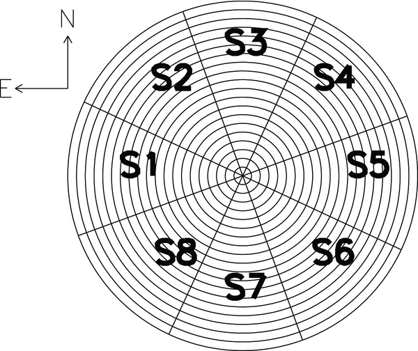
Figure 6. Schematic reseau plot used for the star counts. The radial surface densities were measured in concentric annuli with a width of 05. In order to derive the surface density profile for a different direction, we divided each annulus into eight angular sections (S1–S8).
Download figure:
Standard image High-resolution imageThe stars in the inner part of the cluster are not resolved enough to derive the number density profile because of crowding in the inner section. Thus, we derived the surface brightness (μ) from the center to the outer region and combined this with the number density profile. First, we removed the stars outside the mask envelope (see Figure 3) determined in C–M mask filtering from the J short-exposure image in order to minimize field star contamination. Then, the image was divided into concentric apertures with 025 width in the central region (r < 15) and 05 width in the outer region (r > 15). Each aperture was also subdivided into eight subsections with an angle of 45°, as shown in Figure 6. The mean surface brightness of a given aperture was measured by averaging the surface brightness of eight subsections. In order to correct for the bright star effect, we rejected the subsections with brightness deviating from the mean surface brightness by more than 2σ, then measured the mean surface brightness again using the remaining subsections. The surface brightness profile was finally converted into a number density log (N(r)) using Equation (5):

where C is an arbitrary constant to match number density profile and surface brightness profile. The resulting radial surface density profile is shown in the upper panel of Figure 7, along with a theoretical King model of c = 1.67 (Trager et al. 1995), which was arbitrarily normalized to our surface density profile. We also plotted the photometric recovery rates to consider radial crowding effects on the observed profile. In order to compare our radial profile with previous results, we overplotted the surface brightness of Trager et al. (1995).

Figure 7. Upper: radial surface density profile of NGC 6626 with a theoretical King model of c = 1.67 (thin solid curve), and radial completeness and its trend (dotted line). The open squares represent the surface number density profile converted from the surface brightness profile of Trager et al. (1995). The filled points and cross points are the derived number density and surface brightness profile in this study, respectively. The arrow indicates the tidal radius of NGC 6626. The profile within the detected overdensity region, from log (r'') = 1.9 to log (r'') = 2.6, is represented by a power law, specifically, a thick solid line in logarithmic scale with a slope of γ = −0.80 ± 0.04. The mean number density of stars in the overdensity region is estimated as μ = 0.035 arcsec−2. Lower: radial surface density profiles of eight different angular sections (S1–S8). For clarity, the surface densities from S1 to S8 are given zero-point offsets with values of const. = 0.0, 1.2, 2.5, 3.8, 5.2, 6.7, 8.1, and 9.5. The dotted lines at the end of the King profile mean that King profile continues until the tidal radius. The other notations are the same as those of the radial surface density profile in the upper panel.
Download figure:
Standard image High-resolution image
It is apparent in the upper panel of Figure 7 that the surface brightness profile connects smoothly to the number density profile in the outer region. Furthermore, both radial surface density profiles show an overdensity feature that departs from the King model with a break in the slope at a radius of log (r'') ∼ 1.9 (≈ 0.13 rt) and extends to the radius of log (r'') ∼ 2.6 (≈ 0.62 rt). The radial surface density profile in this overdensity region is described by a power law with a slope γ = −0.80 ± 0.04, which is shallower than the case of γ = −1 predicted by Johnston et al. (1999). A shallower slope than the theoretical one can be explained by the contamination of background stars. Combes et al. (1999) explained that due to the contamination of the background–foreground population, the slope in the observed radial profile could be much shallower than in the simulation. However, we note that the shallow radial profile was not just generated by the contamination of the background field stars. The contamination of the background field stars in this result is relatively insignificant because (1) we gave different weights to stars and subtracted the remaining background density when we derived the radial profile, so that the contamination of the background field stars was somewhat reduced, (2) our survey region only covers the tidal radius of the cluster, so that it is hard to imagine that serious density structures of background stars exist in our survey region, and (3) the surface density of field populations hardly seems to decrease with the distance from the cluster center, even if there are density structures of background field stars larger than the survey region. Indeed, globular cluster NGC 5053, which has been known to have a tidal tail (Chun et al. 2010), also shows a radial profile with a shallower slope than γ = −1. Thus, the components in the shallow overdensity region might be the tidally extended cluster stars and some field stars. In order to more accurately ascertain the effect of the contamination of background field stars, we need to observe a larger field.
Another interesting finding is that the observed radial surface density profiles differ greatly from the shape of the radial profile obtained from the surface density profile of Trager et al. (1995). We attribute the different shape between our observed radial profiles and the previously published profile to the inhomogeneity, poorness, and different limiting magnitudes of the Trager et al. (1995) data. Fundamentally, the surface brightness profiles of Trager et al. (1995) were based on inhomogeneous photometric data. They used several photometric CCD, photographic, photoelectric, and electronographic data obtained from different telescopes. In order to construct a smooth profile, different by-eye weights were assigned to the individual data, then surface brightness profiles were derived by executing iterative polynomial fitting. The relatively poor data quality of Trager et al. (1995) compared with our WIRCam data is also a possible reason for the difference in the shape of the radial profile. Most of the Trager et al. (1995) data were obtained in optical filters of 1–1.5 m telescopes, and the seeing condition was 2–3 arcsec. Thus, the resolution of Trager et al. (1995) was not as good as in our data, and the high-extinction value across the field of NGC 6626 could have affected the data points. Furthermore, as mentioned in Trager et al. (1995), inaccuracies in the determination of sky background contamination could affect the surface brightness at the outer region. Finally, different limiting magnitudes between our data and the Trager et al. (1995) data may have caused the different shape of the radial profile. Note that Combes et al. (1999) certified in their simulation that low-mass stars were usually stripped from a globular cluster and subsequently form tidal tails or streams. The radial density profile of Trager et al. (1995) was derived mainly through surface brightness, thus low-mass stars could not contribute much to the radial profile because the surface brightness is determined by bright stars above a turnoff point, such as giants and horizontal branch stars. Furthermore, when they derived a radial profile through star counts, they excluded the stars of lower mass below the turnoff point. On the other hand, we derived the radial surface density profile from star counts, including faint low-mass stars below the turnoff point. Thus, we can conclude that this overdensity feature and break in the slope of radial density profile are fairly valid features, and the difference from the surface brightness profile of Trager et al. (1995) was caused by several complicated factors such as inhomogeneity, poor data quality, and different limiting magnitude.
The lower panel of Figure 7 presents our radial surface density profiles of eight angular sections with different directions, as defined in Figure 6. The break at log (r'') ∼ 1.9 and the density excess feature out to log (r'') ∼ 2.6 are common in the profiles for all eight angular sections. The estimated mean surface densities (μ) of the excess feature in angular sections 4, 5, and 6 are higher than the total mean density and those in other sections. Specifically, the slopes (γ) of the power laws in angular sections 4 and 5 seem to be flatter than the mean slope of the radial surface density profile and the slopes in the other angular sections. These density features are in good agreement with the overdensity features extending toward the perpendicular direction to the Galactic plane and the direction of the Galactic center, as shown in the surface density maps of Figure 5. Furthermore, the slope (γ) in angular section 7, where the extended overdensity feature is aligned with the proper motion, is also slightly shallow. However, the mean density of this overdensity feature is not high because this feature is not as strong as the density feature in angular sections 4 and 5, as shown in Figure 5. One can find that the slope of the radial density profile in angular section 3 is also flat, but we also note that this flat slope is the result of the effect of the density in this section being lower than that in the other sections.
Finally, we examined the effect of differential reddening on the radial density profile. Significant differential reddening can lead to misidentification of the cluster stellar population in a specific sky region when we sort the cluster's stars on the C–M plane, and ultimately, we can underestimate the stellar density of that region. Indeed, as shown in the dust map of Figure 5, there is a significant differential reddening of ▵E(B − V) ∼ 0.1. By adopting the maximum reddening variation of ▵E(B − V) ∼ 0.1, we can find that the color reddening in the c1 index is about ▵E(c1) = 0.05 and absorption in the Ks magnitude is about  . The reddening and absorption do not cause serious misidentification of cluster stellar population in the grid of the C–M plane. Therefore, we conclude that our radial surface density profile of eight angular sections was not significantly affected by differential reddening.
5. DISCUSSION AND CONCLUSION
From the analysis of the stellar density distribution around the globular cluster NGC 6626 in the previous section, we found that stellar density configurations within the tidal radius are strongly distorted and show extended features. Notable findings include the fact that the stellar elongations tend to extend toward the Galactic center and perpendicular direction to the Galactic plane from the center of the cluster out to the tidal radius. Marginal extensions in the south direction, which are aligned with the projected proper motion, are also revealed near the tidal radius. These asymmetric features and multi-elongations imply complex tidal interaction with the Galaxy, such as tidal force and shock of the bulge and disk that the cluster experienced; this is why the overdensity features commonly appear in all directions. The proximity to the Galactic bulge and disk, 2.7 kpc from the Galactic center and 0.5 kpc from the Galactic plane (Harris 1996), increases this probability. In the recent work on the morphological study of globular clusters by Chen & Chen (2010), they indeed reported that NGC 6626 exhibits obvious flattening in shape the elongation of which points to the Galactic center due to the tidal effect of the bulge.
The strong tidal effect with the Galaxy and the extratidal feature of NGC 6626 could give a hint into the origin and evolution of this cluster. NGC 6626 is a metal-poor globular cluster with [Fe/H] = −1.32 (Harris 1996), which is not significantly different from that of metal-poor clusters in the outer halo. However, its location near the metal-rich bulge region and the thick-disk-like orbit (Cudworth & Hanson 1993) present a question of whether or not this cluster is a classic halo cluster. Based on the cluster's compactness, Davidge et al. (1996) suggested that NGC 6626 is not merely a passerby from the outer halo but it has indeed been a habitant in the bulge region for a long time. Dinescu et al. (1999) suggested two possibilities regarding the origin of NGC 6626: accretion from the satellite galaxies that merged into the Milky Way and formation in a metal-poor gaseous disk, which is a rotationally supported system. More recently, Lee et al. (2007) found that globular clusters with EHB stars are kinematically decoupled from the normal clusters. They classified NGC 6626 as an EHB globular cluster and suggested that this cluster, which has a low total orbital energy Etot, could be a remnant of the first building blocks that assembled in the early universe. Making an inference from our result of tidal stripping stellar features and the previous results cited above, we could attribute the extraordinary properties of NGC 6626 in dynamics, i.e., thick-disk-like orbit and low Etot, to the dynamic interaction with the Galaxy. Furthermore, if we take the first possible origin from Dinescu et al. (1999) and the suggestion of Lee et al. (2007), we could interpret that the globular cluster NGC 6626 would have been formed in the primordial first building blocks that are thought to have merged and formed the bulge region in the early universe; the subsequent dynamical interaction with the Galaxy that the cluster underwent in the process of accretion brought about its extraordinary dynamical properties, such as a disk-like orbit motion and the low Etot that we see in the present day.
It is also worth noting that the accretion scenario described above is not significantly different from the predicted process of galaxy formation in the hierarchical merging paradigm. According to the hierarchical merging paradigm of galaxy formation, the formation of galaxies in the early stage involves a series of merging events of subgalactic clumps, such as large satellite galaxies (Baugh et al. 1996). In particular, the Milky Way bulge region experienced active merging events in the early universe and formed through a short series of starbursts triggered by gas-rich mergers (Zoccali et al. 2006). In this merger process, the number of bulge stars were accreted from infalling satellite galaxies and formed through star formation triggered by the mergers (Katz 1992). Indeed, chemical and dynamical evolution studies of the bulge region, such as the study of Nakasato & Nomoto (2003), showed that the accretion and starburst of early mergers contributed to some parts of the metal-poor stars and to the wide metallicity distribution in the bulge region. They noted that these bulge stars become substantially rotationally supported through the loss of angular momentum by tidal friction during the merging process. Furthermore, Rahimi et al. (2010) found that the metal-poor stars accreted from large satellite galaxies that merged into the main galaxy in an early epoch may have low total energy Etot because of dynamical friction. Satellite galaxies such as Sagittarius (Bellazzini et al. 2003; Tautvaišienė et al. 2004; Sbordone et al. 2005) and Fornax (Buonanno et al. 1998, 1999) also have their own globular clusters, and thus in the merging process of satellite galaxies, the metal-poor globular clusters could be captured into the bulge region and have low Etot and rotational orbit motion, as metal-poor stars do. This has many analogs in the suggestion of Côté et al. (1998) that the metal-poor clusters were captured from other galaxies through merger and tidal stripping. Therefore, the scenario explained, in which NGC 6626 formed in a satellite galaxy that merged into the Milky Way in the early universe and was subsequently captured with the modification of dynamical properties, is not implausible.
Nonetheless, we cannot exclude the possibility that NGC 6626 formed in rotationally supported metal-poor gas, which existed fairly early in the thick disk. The thick-disk orbit property of NGC 6626 increases this possibility further. Indeed thick-disk stars are generally considered to be older and more metal poor than their bulge counterparts (Majewski 1993; Chiba & Beers 2000; Bochanski et al. 2007), and a significant fraction of metal-poor thick-disk stars has been identified in the disk field (Norris 1996; Beers & Sommer-Larsen 1995; Chiba & Yoshii 1997). Several studies (Elmegreen & Elmegreen 2006; Bournaud et al. 2009) on thick-disk formation also noted that most thick-disk stars may have formed in a rotationally supported system in the galaxy itself. Thus, as Dinescu et al. (1999) mentioned, massive clumps, where thick-disk stars might form, could generate globular clusters. In this case, the globular clusters also experience strong tidal interaction with the bulge and disk. For a globular cluster originating in the thick disk, however, it is not obvious that the tidal features perpendicular to the galactic plane would be able to be constructed around the cluster because it would experience a varying right(z)-component of the galactic plane potential less than the cluster passing the galactic plane from outer region. Additional studies of stellar density configuration of globular clusters in the disk and bulge regions are necessary.
It is meaningful to estimate the time at which the cluster was affected by the last disk-shock effect to understand the origin of NGC 6626 in more detail. Using the velocity dispersion of NGC 6626 obtained by Pryor & Meylan (1993), Equation (5) of Peñarrubia et al. (2009), and position of the break radius in our radial profile, we could find that NGC 6626 experienced disk shock in the last half of the orbit period (one orbit period is about 75 Myr; Dinescu et al. 1999). However, we are not sure whether the stars in the extended feature were really stripped by the last disk shock. The stars in the extended features could have been stripped by a previous disk shock. Although the orbit period of the cluster is so short that the cluster could not survive the tidal interaction with the external fields for many orbits in the inner galactic region, Miocchi et al. (2006) confirmed that the clusters with high concentration (c > 1.6) can survive the tidal interaction up to complete orbital decay (t ∼ 300tb, where tb is the galaxy core crossing time) in the inner region of the galaxy. Indeed, the present concentration (c) of NGC 6626 is about 1.67 (Trager et al. 1995), thus the cluster and its tidal substructure could remain in the vicinity of the cluster. Numerical simulation of a globular cluster on the NGC 6626 orbit is necessary to further understand the process of its origin and evolution.
In summary, we have examined the spatial density distribution of the stars within the tidal radius of the metal-poor globular cluster NGC 6626 in the Galactic bulge region, using wide-field (∼21' × 21') near-infrared J, H, and Ks images of the WIRCam detector. Two-dimensional surface density maps showed that stellar density configurations are strongly distorted and appear as extended density features. The observed extensions likely trace the spatial orbits of the cluster, as well as the effects of dynamical interaction with the Galaxy. Radial surface density profiles also represent the overdensity feature with a break in the slope within the tidal radius. We note, however, because our field of view is narrow and several field stars could be involved, that the results of this study need to be reconfirmed in further investigation. In this study, we also tried to discuss the origin and evolution of NGC 6626 from the extratidal features around the cluster. Based on our results and previously published findings, we could interpret that NGC 6626 might be a remnant of the first building block that merged and formed the bulge region in the early universe. However, the possibility of originating from a primordial and rotationally supported system in a thick disk still remains open. Wider field photometric data and a more accurate proper motion of clusters are essential to more accurate verification of our results. Furthermore, additional studies of stellar density configuration for metal-poor and metal-rich clusters in the Galactic bulge region should also be required. If we find additional extratidal substructure for other globular clusters in the Galactic bulge and disk region and spatial coherence between tidal structures, we could understand the formation of metal-poor clusters in the bulge and disk region in the galaxy merging paradigm. Unfortunately, thus far, there have been few studies of the stellar density distribution of globular clusters in the bulge and disk region. Thus, we expect that our results can provide constraints to interpret not only the origin of metal-poor clusters in the Milky Way bulge region but also the formation of the bulge region in the Milky Way.
We are grateful to an anonymous referee for a detailed report that greatly improved this paper. This research was supported by Basic Science Research Program through the National Research Foundation of Korea (NRF) funded by Ministry of Education, Science and Technology (2010-0021867). This work is partially supported by the KASI-Yonsei Joint Research Program (2010-2011) for the Frontiers of Astronomy and Space Science funded by the Korea Astronomy and Space Science Institute.