


ABSTRACT
This paper studies the orbital dynamics around the main-belt asteroid Kleopatra through a detailed look at the motion around the equilibria using observational data. The shapes of zero-velocity surfaces are represented at assigned values of the Jacobi integral to explore the connections between forbidden regions in three-dimensional space and the final fates of the nearby trajectories. All four equilibria are found to be nonlinearly unstable, and the degree and mode of instability are further clarified by decomposing the motion into respective local manifolds. This study suggests that there are many sensitive and uncertain trajectories near the equilibria due to the multiplicity of unstable branching trajectories around the center manifolds. Six continuous major families of periodic orbits are obtained close to the equilibria, which are proved to be unstable by Floquet theory.
Export citation and abstract BibTeX RIS
1. INTRODUCTION
Recently, numerous space missions have sent deep space probes to asteroids, comets, and planetary satellites (Kawaguchi et al. 2008; Russell et al. 2007), indicating an increasing interest in the study of small bodies in the solar system. These missions perform extremely challenging tasks such as close proximity operations on or around these small bodies. Such actions are also the key technologies to be demonstrated in some current missions (e.g., NASA's Dawn mission and Hayabusa 2 by JAXA). It is an established fact that small bodies are diverse in terms of shape, rotational state, size, density, and spin rate (Hilton 2002; Pravec et al. 2002), making the dynamics about every small body both unique and complicated, especially in the vicinity of their surfaces. Thus, proper approaches to characterize and evaluate the orbital dynamics about these small bodies are necessary and provide remarkable information for successful mission planning in general.
The irregular gravitational fields induced by small bodies add new complexity to classical celestial dynamics. Generally, these gravitational fields are noncentral and asymmetrical vector fields with zero divergence and vorticity; in such a case, some trajectories can exhibit strongly unstable and chaotic motion near the surface of the small bodies (Scheeres et al. 1998). Previous studies used to start with some simple specific geometric objects; for instance, a group of small bodies with an elongated shape could simply be modeled as a finite line segment (Riaguas et al. 1999), and triaxial ellipsoids are more frequently used for asteroid gravity approximation (Scheeres 1994). Werner & Scheeres (1997) developed a polyhedral method that describes the gravitational field of a constant density polyhedron and can precisely evaluate the gravitational field around a specific asteroid. This method has been recently applied to the investigation of close orbit dynamics around the non-principal-axis rotator 4179 Toutatis (Scheeres et al. 1998) and the evaluation of the actual dynamical environments around 433 Eros and 25143 Itokawa (Scheeres et al. 2000, 2006).
The dynamics in the vicinity of the main-belt asteroid 216 Kleopatra is paid attention to for the following reasons: first, its puzzling dog bone shape induces a dominant second-degree and -order gravitational field. Since Kleopatra is much more massive than many near-Earth asteroids, its natural orbital motion is mainly determined by this irregular field. Second, the relatively high spin rate of Kleopatra indicates a strong possibility of resonance occurrence, which can have a crucial effect on the orbital pattern. Last, the study of the dynamics around Kleopatra might be representative of similarly elongated asteroids, such as 4769 Castalia, 4179 Toutatis, 243 Ida, 433 Eros, and 113 Amaltea.
In this paper, the dynamical processes close to the asteroid Kleopatra are investigated by examining the orbital structure at and around equilibrium, as well as nearby periodic orbits, using observed values of physical parameters. First, the general properties of Kleopatra are discussed in Section 2 as well as the evolution of a three-dimensional zero-velocity surface with regard to a classification of the orbits around Kleopatra by the integral constant. In Section 3, the equilibrium manifolds are presented to clarify the orbital structure around the equilibria, and the effects of the three types of local manifolds are also included into the discussion on the instability and departing trajectories at the equilibria. Section 4 deals with the stability of the periodic orbits around the equilibria, especially regarding the degree of instability for different orbit families and the dependence on corresponding equilibria.
2. GEOMETRIC PROPERTIES AND MODEL OF KLEOPATRA
The physical model of Kleopatra's shape adopted in this paper was derived based on the radar observations and optical light curves obtained by Ostro et al. (2000). As illustrated in Figure 1, a polyhedral model with 2048 vertices and 4096 faces was established by Ostro et al. (2000) using the least-squares inversion method, which quantitatively estimates Kleopatra's shape and provides the basic data to approximate the asteroid's gravitational field with overall dimensions of 217 × 94 × 81 km and a volume of 7.09 × 10⁵ km3. Assuming Kleopatra is homogeneous, the bulk density is 3.6 ± 0.4 g cm−3, which is derived from the total mass of the asteroid, 4.64 ± 0.02 × 10¹⁸ kg, as determined from long-term accurate measurements of its satellite orbits (Descamps et al. 2011).

Figure 1. Shape of the Kleopatra model viewed from ±x-, ±y-, and ±z-axis directions. The topography elongates in the x-direction and surprisingly bulges at both ends, a shape which has been described as a dog bone or a dumbbell in previous literature (Descamps et al. 2011).
Download figure:
Standard image High-resolution imageTwo coordinate systems will be used throughout this paper. The first is an inertial frame with axes labeled X, Y, and Z. The Z-axis is parallel to the primary rotation axis of Kleopatra, which is averaged and given in J2000 ecliptic coordinates by λ = 76° ± 3° and β = 16° ± 1° (Ostro et al. 2000). The other coordinate system is a fixed frame labeled x, y, and z with the origin located at the Kleopatra model's center of mass. The x-, y-, and z-axes correspond to the principal axes of the smallest, intermediate, and largest moments of inertia, respectively, Jx, Jy, and Jz, whose values are as follows:
The relationship between the gravity coefficients and the principal moments of inertia is taken into account, giving the following values of normalized second-degree and -order gravity coefficients with the reference radius 143.388 km:
Hu & Scheeres (2004) introduced the mass-distribution parameter σ, a simple measure of an asteroid's shape and gravity field with dynamical implications, where σ = (Jy − Jx)/(Jz − Jx). For Kleopatra, σ ∼ 0.99, indicating this asteroid is very close to having a prolate shape. This is demonstrated in Figure 2, which shows a topographic map of Kleopatra based on the polyhedral model; the dominant second-degree and -order gravitational field can clearly be seen around it.

Figure 2. Topographic map of Kleopatra (unit: km).
Download figure:
Standard image High-resolution imageThe rotational period of Kleopatra was optically determined to be 5.385 hr (Ostro et al. 2000). Since a high-speed uniform rotational state implies a stable and permanent rotation around the principal axis of the largest moment of inertia, we will assume that Kleopatra rotates uniformly about the z-axis of the body-fixed frame.
3. THE EQUATIONS OF MOTION AND CONSERVATION
The analysis of the motion in this non-central irregular gravitational field is based on the equations of motion in the body-fixed frame; these equations are well defined by the appearance and rotational state of the Kleopatra model. Since the motion of spacecraft relative to the asteroid will be affected by, for example, radiation pressure and the gravitational pull of the Sun or a major planet, the gravitational environment in the vicinity of Kleopatra is preliminarily estimated. For Kleopatra, the major perturbation comes from the solar gravity; these effects can be delimited in the terms of the Hill sphere (Hamilton & Burns 1992), which gives a dimension of 2.89 × 10⁴ km, much larger than that of the asteroid. Therefore, orbital motion in the vicinity of Kleopatra is dominated by its own gravitational field, which allows us to neglect any gravitational pull from remaining bodies in this paper.
In the polyhedral method, the exterior potential, attraction, and gravity gradient matrices are derived as closed forms and computed by a FORTRAN code. The adaptive step size Runge–Kutta method (order of 7–8) was adopted for the numerical integration of the equations of motion. A fast and effective algorithm was also employed to calculate the polyhedral mass properties of Kleopatra (Mirtich 1996).
3.1. Equations of Motion and Canonization
For a gravitational field and rotation state as stated above, Scheeres et al. (1998) presented the complete form of the equations of motion in the body-fixed frame as

where r is the body-fixed vector from the original point to the field point, ω is the angular velocity (a constant vector in the inertial frame), U(r) is the gravitational potential, −∇U(r) is the gravitational attraction, ∇ is the gradient operator, and the operators  and
and  represent the first- and second-order time derivatives with respect to the body-fixed-body frame.
A definition of efficient potential (2) was introduced in order to combine Equations (1) and (2) into Equation (3) (Scheeres et al. 1998):

Equation (3) is conserved because the Coriolis term  has no effect and the term −∇V(r) is potential force; thus, the divergence of Equation (3) is zero. Furthermore, it can be proved that Equation (3) describes a Hamiltonian system by means of Legendre transformation (Arnold 1989, p. 61); it retains a symplectic form and conserves phase volume in each extended phase space, resulting in unpredictability of long-term dynamical behaviors.
An integral of generalized energy exists due to the explicit time independence of the Hamiltonian function, which is expressed as

Therefore, the value of the Hamiltonian function is constant for all the motion with the same initial conditions, and the constant C is called the Jacobi integral.
3.2. Zero-velocity Surfaces
The definition of the Jacobi integral enables a variety of initial conditions to lead to the same integral value; this serves well for the classification of the natural orbits around an asteroid. As reported in previous studies (Szebehely 1967, p. 164), Equation (4) establishes a well-defined region in the body-fixed frame for each of the orbit categories. The whole space is divided into an allowable region, V(r) ⩽ C, and a forbidden region, V(r) > C, based on the determined integral value. The boundary of these regions is governed by V(r) = C, which is known as the zero-velocity surface. The geometry and topology of these surfaces could have several intentional effects on the dynamical behaviors of the system. Figure 3 demonstrates the zero-velocity surfaces around Kleopatra with different values of the Jacobi integral.

Figure 3. Zero-velocity surfaces with different values of the Jacobi integral C (in km2 s−2): C1 = −2.5719 × 10⁻³, C2 = −2.4719 × 10⁻³, C3 = −2.1719 × 10⁻³, C4 = −1.9909 × 10⁻³, C5 = −1.9459 × 10⁻³, and C6 = −1.6459 × 10⁻³.
Download figure:
Standard image High-resolution imageWhen C < 0, the vicinal initialized orbit may collide with and rebound off of the zero-velocity surface, suffering a final fate of conversion. On the other hand, when C ⩾ 0, the forbidden region shrinks and fades away, implying globally accessible exterior space. In detail, when C = C1, the zero-velocity surface consists of two branches—an inner one that clings to and entirely wraps around the asteroid and an outer one that is cylindrical. Here, the allowable region is divided into two parts: orbits initialized in the outer branch will never approach the asteroid, whereas those initialized in the inner branch will end up colliding with the asteroid. These two branches begin to connect as the integral increases in value (C1 < C < C2); the allowable regions merge into one, and the outer and inner orbits move to the side through the neck area. The zero-velocity surface splits into two branches again around C = C5, with the upper branch and lower branch dividing the forbidden region into two parts. This indicates that all orbits near the equatorial plane are probable at this time (C > C5).
4. EQUILIBRIA, NEARBY PERIODIC ORBITS, AND STABILITY
Previous investigations of dynamic environments around uniformly rotating and elongated asteroids, such as 433 Eros and 4796 Castalia, found four equilibria about them (Scheeres et al. 1996, 2000). These equilibria are the critical points where the zero-velocity surfaces get self-intersected. Figure 4 illustrates the equilibria and the contour lines of the Jacobi integral in the equatorial plane (z = 0). The four equilibria around Kleopatra are roughly located in the equatorial plane and symmetrical about the x = 0 and y = 0 axes.

Figure 4. Zero-velocity curves in the equatorial plane (z = 0).
Download figure:
Standard image High-resolution imageThe values of the equilibria are obtained by solving Equation (5) and are displayed in Table 1.

The equilibria represent stationary orbits in the inertial frame that remain above particular spots on the asteroid surface. The existence of these natural stationary orbits depends on the stability of these points. The linearization method is applied to examine the stability of the equilibria (Szebehely 1967, p. 238); this method describes the state equations in perturbation form in the neighborhood of the equilibria:

Table 1. Exact Locations of the Equilibria
| Equilibrium Point | x | y | z |
|---|---|---|---|
| (km) | (km) | (km) | |
| E1 | 142.8443 | 2.4414 | 1.1818 |
| E2 | −144.6762 | 5.1889 | −0.2726 |
| E3 | 2.2304 | −102.0919 | 0.2719 |
| E4 | −1.1637 | 100.7297 | −0.5460 |
Download table as: ASCIITypeset image
Here,  is the perturbation state variable, A is the coefficient matrix of the linearized system, and
  is a small quantity of the same order of
  . The eigenvalues of matrix A are obtained by solving
  and are shown in Table 2.
Table 2. Eigenvalues of the Coefficient Matrix of the Linearized System
| Eigenvalue | E1 | E2 | E3 | E4 |
|---|---|---|---|---|
| (×10−3) | ||||
| λ1 | 0.3761 | −0.4225 | 0.2022+0.3040i | 0.2018+0.3061i |
| λ2 | −0.3761 | 0.4225 | 0.2022–0.3040i | 0.2018–0.3061i |
| λ3 | 0.4251i | 0.4665i | −0.2022+0.3040i | −0.2018+0.3061i |
| λ4 | −0.4251i | −0.4665i | −0.2022–0.3040i | −0.2018-0.3061i |
| λ5 | 0.4134i | 0.4135i | 0.3270i | 0.3227i |
| λ6 | −0.4134i | −0.4135i | −0.3270i | −0.3227i |
Download table as: ASCIITypeset image
Equilibria E1 and E2 possess two real eigenvalues (one positive and one negative) and two pairs of purely imaginary ones, while equilibria E3 and E4 possess two pairs of conjugate complex eigenvalues and one pair of purely imaginary ones. Generally, each of these four equilibria possesses at least one eigenvalue with a positive real part. Therefore, all of the four equilibria are linearly unstable, which also makes the original nonlinear system (3) unstable at the equilibria by means of Lyapunov's second method (Szebehely 1967, p. 238). This instability makes Kleopatra a Type II asteroid, according to the categorization by Scheeres (1994).
Additionally, this conclusion also corresponds to the criterion on the stability of equilibria in a uniformly rotating arbitrary second-degree and -order gravitational field (Hu & Scheeres 2008), which states that the equilibria E1 and E2 are always unstable, and the stability of E3 and E4 are subject to

For Kleopatra, the index on the left-hand side of Equation (7) is −3.198, which violates the condition in Equation (7) and is consistent with our above analysis.
4.1. Equilibrium Manifolds
The equilibrium manifolds are investigated in this section in order to determine the motion around the equilibria and to estimate the complexity of the global structure of the orbits in general. The four equilibria all possess eigenvalues with positive, negative, and zero real parts at the same time; namely, they are non-hyperbolic. Thus, the local invariant manifolds in the neighborhood of these equilibria include not only the stable and unstable manifolds, but also the center manifolds. This combination of equilibrium manifolds adds new complexity to their behaviors, especially on the center manifolds, which enables the existence of dense periodic orbits around the equilibria, as discussed below.
First, the structure of the invariant subspaces induced by the linear part of the system (6) is determined. Specifically, the eigenvalues demonstrated in Table 2 with positive, zero, and negative real parts determine the stable (E s), central (E c), and unstable (E u) subspaces, respectively. These subspaces are expanded by the eigenvectors affiliated with the corresponding eigenvalues, satisfying R6 = Es⊕Ec⊕Eu. The subspaces are described in the following manner:
where vs is the eigenvector of the eigenvalue with a negative real part, vu is the eigenvector of the eigenvalue with a positive real part, and vc is the eigenvector of the purely imaginary eigenvalue. The complex conjugate vector bases are replaced by the real and imaginary parts of these vectors.
Since the local manifolds are tangent to their corresponding invariant subspaces at the equilibria, an iterative method was applied in order to approximate the local invariant manifolds around the equilibria that were initialized at the solutions of the linearized system. The center manifold theorem ensures the unique existence of local stable and unstable manifolds of the same dimensions as Es and Eu, and the existence of a local center manifold with the same dimension as Ec.
For equilibria E1 and E2, the dimension of subspaces E s, E c, and E u are respectively 1, 4, and 1, based on the number of corresponding bases. Figure 5 illustrates the one-dimensional local stable and unstable manifolds of E1 and E2, which are tangent to the hyperbolic subspaces and form a saddle manifold. Nearby orbits will approach E1 and E2 logarithmically or displace them exponentially along their respective manifolds. For E1, the characteristic times of the stable and unstable manifolds are both 0.74 hr; for E2, these values are both 0.66 hr.

Figure 5. Segments of stable and unstable local manifolds of the E1 and E2 equilibria (the projection in body-fixed configuration space). Stable manifolds are blue lines, and unstable manifolds are red lines.
Download figure:
Standard image High-resolution imageMini periodic orbits around E1 and E2 are guaranteed to exist by the local manifolds, which are not unique objects and do not possess corresponding dimensions. Two basic quasi-elliptical families of periodic orbits in close vicinity to E1 and E2 are obtained by direct prolongation of the linearized periodic solutions affiliated with the minimum center subspaces; here, the subspaces are expanded by a pair of eigenvectors that correspond to purely imaginary eigenvalues. These local center manifolds are two-dimensional and are tangent to their corresponding minimum center subspaces, as Figure 6 illustrates. Calculations show that the exact values of the periods are quite close to the periods of the corresponding linearized systems, which are 4.11 hr (blue) and 4.22 hr (red) for E1, and 3.74 hr (blue) and 4.22 hr (red) for E2.

Figure 6. Two segments of the local center manifolds of E1 and E2, including the prime periodic orbit families, projected in the body-fixed configuration space.
Download figure:
Standard image High-resolution imageFigure 7 shows the local stable and unstable manifolds of E3 and E4, which are two-dimensional objects tangent to the invariant subspaces and constitute spiral manifolds. The red surfaces in Figure 7 represent the unstable manifolds, in which the trajectories move exponentially away from the equilibrium in a spiral pattern. The blue surfaces represent the stable manifolds, in which the trajectories exponentially approach the equilibrium in a spiral pattern. The characteristic times for E3 and E4 are 1.38 hr and 1.37 hr, respectively, and the spiral period is about 5.7 hr.
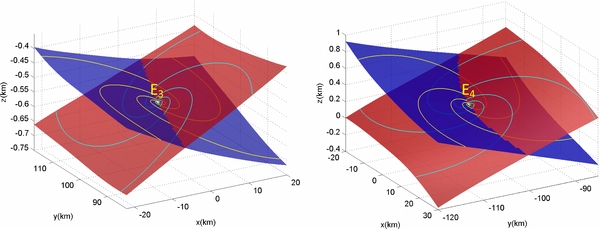
Figure 7. Local stable and unstable manifold patterns of E3 and E4, projected in the body-fixed configuration space. The blue surfaces are the stable manifolds, on which the trajectories spiral inward exponentially; the red surfaces are the unstable manifolds on which the trajectories spiral outward exponentially.
Download figure:
Standard image High-resolution imageUnlike E1 and E2, only one pair of purely imaginary eigenvalues exists for E3 and E4; this imaginary pair gives two-dimensional center subspaces with the linearized periods 5.41 hr and 5.34 hr, respectively. As Figure 8 illustrates, corresponding periodic orbit families are obtained close to these equilibria, forming two-dimensional center manifolds tangent to the center subspaces; here, the values of the periods are approximately equal to the linearized periods.

Figure 8. Segments of the local center manifolds of E3 and E4, projected in the body-fixed configuration space.
Download figure:
Standard image High-resolution imageThe descriptions of the local manifolds around the equilibria E1–E4 suggest the decomposability of their orbital motion; the component in stable manifolds approaches the equilibria logarithmically, the component in unstable manifolds departs from the equilibria exponentially, and the component in center manifolds repeats periodic motion along a quasi-elliptical orbit. These descriptions also indicate that the instability of motion around the equilibria is due to the unstable manifold, wherein even slight perturbations propagate exponentially in time. In practice, the motion initialized in the stable or center manifolds may fail at any time due to random and regular perturbations in space, perturbations that are uncertain due to the multiplicity of nearby unstable branches. Nevertheless, the four non-hyperbolic equilibria E1–E4 can be classified into two types by the dimensions of their local manifolds, which are related to the different modes of the orbits in the vicinity of the asteroid. First, the unstable spiral manifolds at E3 and E4 dominate the orbits near the equatorial plane, which spiral in the opposite direction of the asteroid's rotation. Second, the orbits near E1 and E2 are dominated by the direct unstable manifolds and thus gain greater departing speed. Loopy Lissajous orbits exist in the center manifolds of E1 and E2 because of the hybrid periodic orbit families about, while around E3 and E4, periodic orbits are monotonous and quasi-elliptic.
4.2. Nearby Periodic Orbits and Their Stability
Differing from the equilibria, periodic orbits in the body-fixed frame have limited periods and non-point trajectories, which enable quantitative evaluation of the stability. Generally, periodic orbits in the inertial frame are not periodic orbits in the body-fixed frame, except in a resonance situation (Scheeres et al. 2000); thus, the majority of periodic orbits in the inertial frame are instantaneous and temporary, even without perturbations. Hu & Scheeres (2004) revealed a close relationship between the stability of equilibria and that of their nearby periodic orbits under planar second-degree and -order gravity fields. In this section, the periodic orbits around the equilibria are searched in a wider context, which may not exactly represent the local center manifolds, but these orbits are still delimited by the linear regime. These critical orbits are obtained by continuously searching the center subspaces stated above, which are initialized with periodic solutions of variable sizes. The initial iterative value is chosen as kvc, where k is the size of orbit and vc is the basis of the corresponding center subspaces. Figure 9 illustrates the six families of periodic orbits emerging from the equilibria E1–E4, as obtained through the search with eigenvectors.

Figure 9. Periodic orbits around equilibria E1–E4, obtained with the initial dimension parameter k from 0.1 km to 3.0 km. The locations of the equilibria are marked by a cross. The blue lines are the short-period orbits and the red lines are the long-period orbits.
Download figure:
Standard image High-resolution image
The period ranges of these orbits are listed in Table 3 with the characteristic times of their corresponding linear subspaces; the two times are quite similar for all the equilibria, as shown below.
Table 3. Period Range and Characteristic Times for the Orbit Families
| Orbit Family | Equilibria | Characteristic Time | Range of Period |
|---|---|---|---|
| (s) | (s) | ||
| 1 | E1 | 14781.9386 | 14780.8207–14781.9386 |
| 2 | E1 | 15198.9781 | 15180.5852–15198.9781 |
| 3 | E2 | 13467.9762 | 13468.0596–13473.1415 |
| 4 | E2 | 15195.0386 | 15101.3473–15194.6814 |
| 5 | E3 | 19211.9654 | 19211.9685–19213.1285 |
| 6 | E4 | 19468.5788 | 19468.6284–19469.0286 |
Download table as: ASCIITypeset image
These six orbit families generally expand from their respective center manifolds at the equilibria, but there are a few exceptions. As mentioned above, loopy periodic orbits are probably found around E1 and E2, leading to a hybrid of the two modes of vibration, while in reality, these two natural periods are so close that it is difficult to reduce the ratio to a simple value. In fact, the ideal Lissajous orbit would possess extremely long periods and would be extremely difficult to form due to the unstable manifolds. In addition, modes of vibration exist for the four equilibria which are roughly perpendicular to the equatorial plane. Last, the shape of the periodic orbits around E1 and E2 are quasi-elliptic, while the periodic orbits around E3 and E4 have a three-dimensional bean-like shape with the concavity toward the asteroid.
The Floquet theorem (Perko 1991) is applied to determine the stability of these periodic orbits. This theorem deals with a periodic coefficient linear system, which is obtained by linearizing the original system in Equation (3) along a specific orbit (Hu & Scheeres 2008). Here, the periodic coefficient matrix A(t) is six-dimensional, thus the criterion for the planar case will not work. The monodromy matrix M = Φ(t0 + T, t0) is defined as the solution to the state transition matrix for one period (Montagnier et al. 2004), which is solved in this section tracking every periodic orbit; it indicates the propagation characteristic of the perturbations along an orbit. The stability of the periodic orbits is determined by calculating the eigenvalues of M; if the maximum norm of the eigenvalues is greater than one, ||λ||max > 1, the orbit is unstable; otherwise, if ||λ||max < 1, the orbit is stable. Finally, ||λ||max = 1 represents the critical case.
Table 4 lists the ranges of the exact values of ||λ||max for the six orbit families, which shows that all six families of periodic orbits are unstable. Moreover, these values measure the instability of these orbits, which largely rests with the instability of the equilibria: the periodic orbits around E3 and E4 show less instability than those around E1 and E2.
Table 4. Ranges of Exact Values of ||λ||max
| Orbit Family | ||λ||max | Stability |
|---|---|---|
| 1 | 259.0902–259.8178 | US |
| 2 | 301.8484–305.3634 | US |
| 3 | 291.8076–296.0417 | US |
| 4 | 590.4577–614.1852 | US |
| 5 | 48.5337–48.6166 | US |
| 6 | 50.8036–50.8382 | US |
Download table as: ASCIITypeset image
5. CONCLUSIONS
In this paper, we state significant connections between the topography of the zero-velocity surfaces in three-dimensional space, the equilibrium points, and the orbital structure in the vicinity of Kleopatra. All of the four equilibria proved to be nonlinearly unstable, confirming that natural stationary orbits are absent in this system. By decomposing the motion around these equilibria into respective local manifolds, it further clarifies that E1 and E2, which have saddle manifolds, are more unstable than E3 and E4, which have spiral manifolds. In addition, sensitive and uncertain trajectories were shown to be plenty due to the multiplicity of unstable branching trajectories around the center manifolds. Six continuous major families of periodic orbits were also found close to the equilibria, which were determined to be unstable by the Floquet theory. It is shown that the degree of instability of these periodic families is related to and consistent with that of the corresponding equilibria in this system. These quasi-stationary orbits thus provide a feasible solution for a short-term hovering orbit.
This work was supported by the National Basic Research Program of China (973 Program, 2012CB720000) and the National Natural Science Foundation of China (No. 11072122).