


ABSTRACT
In this paper, we study the ability of CCD- and electron-multiplying-CCD-based speckle imaging to obtain reliable astrometry and photometry of binary stars below the diffraction limit of the WIYN 3.5 m Telescope. We present a total of 120 measures of binary stars, 75 of which are below the diffraction limit. The measures are divided into two groups that have different measurement accuracy and precision. The first group is composed of standard speckle observations, that is, a sequence of speckle images taken in a single filter, while the second group consists of paired observations where the two observations are taken on the same observing run and in different filters. The more recent paired observations were taken simultaneously with the Differential Speckle Survey Instrument, which is a two-channel speckle imaging system. In comparing our results to the ephemeris positions of binaries with known orbits, we find that paired observations provide the opportunity to identify cases of systematic error in separation below the diffraction limit and after removing these from consideration, we obtain a linear measurement uncertainty of 3–4 mas. However, if observations are unpaired or if two observations taken in the same filter are paired, it becomes harder to identify cases of systematic error, presumably because the largest source of this error is residual atmospheric dispersion, which is color dependent. When observations are unpaired, we find that it is unwise to report separations below approximately 20 mas, as these are most susceptible to this effect. Using the final results obtained, we are able to update two older orbits in the literature and present preliminary orbits for three systems that were discovered by Hipparcos.
Export citation and abstract BibTeX RIS
1. INTRODUCTION
In recent years, the use of CCDs and electron-multiplying CCDs in speckle imaging has led to a large number of magnitude differences of binary stars appearing in the literature (see, e.g., Horch et al. 2004, 2010, 2011; Balega et al. 2007; Tokovinin et al. 2010; Docobo et al. 2010). The linearity of these devices has permitted reliable photometric information to be obtained, at least under observing conditions where the decorrelation of primary and secondary speckle patterns due to the finite size of the isoplanatic patch can be assumed to be small. These magnitude differences should eventually pave the way for many robust comparisons with stellar structure and evolution models for the sample of "classic" speckle binaries, i.e., those with separations in the range ∼0.04–1 arcsec, a significant contribution which would not be possible without photometric information of the components in multiple filters.
However, the existence of reliable photometry in speckle imaging has another, perhaps more important, advantage: the ability to determine the shape of the speckle transfer function in detail, or equivalently, the average shape of the individual speckles themselves. For example, if speckles are seen as blended or elongated due to a component below the diffraction limit, it should in theory be possible to retrieve the relevant astrometric and photometric information, if the data are taken with a linear detector. With older microchannel-plate-based systems, systematic errors in detection affect the detailed shape of the speckles obtained, adding a severe complication to the interpretation of the speckle profile. However, with seeing-limited images of high quality taken with linear detectors, it is possible to fit a blended stellar profile to a binary star model with reasonable accuracy. Of course, performing a binary star fit to such a profile is put on much more stable ground if the object is known or suspected to be binary by other means. The same should hold true with sub-diffraction-limited speckle observations of binaries: with linear detectors and high-quality observations, there is no need to view the diffraction limit as an absolute barrier when analyzing speckle data.
Tokovinin (1985) was among the first to realize the possibility of measurement below the diffraction limit in speckle observations using his phase-grating interferometer, and he did so well before linear detectors were widely used for speckle. Other speckle observers have been occasionally tempted to follow his example by reporting measures below the diffraction limit, especially on important binary systems where the measure added information at a key point in the orbital trajectory. Our own earlier work (Horch et al. 2006a) attempted to understand, albeit in a preliminary way, the conditions that permit reliable information to be obtained at such separations. In that work, we showed that if one has linear data in two colors, it is possible to distinguish between residual atmospheric dispersion, which is color dependent, and the presence of a sub-diffraction-limited component, which is not.
In 2008, we built the Differential Speckle Survey Instrument (DSSI), a speckle imaging system that contains a dichroic element so that it takes data in two different filters simultaneously. The instrument itself is described in Horch et al. (2009, hereafter Paper I) and has the following advantages over single-channel speckle imagers: (1) twice as much data are taken per unit of time, which can be used either to increase the signal-to-noise ratio for astrometric measurement or to decrease the time needed to achieve a given signal-to-noise ratio, (2) a color measurement of the components of a binary system can be made in a single observation, and (3) taking data in two colors simultaneously gives leverage on residual atmospheric dispersion, which is especially important for sub-diffraction-limited measurement. The first two items mentioned were discussed more fully in Horch et al. (2011, hereafter Paper II). In the current paper, we study the measurement accuracy and precision obtained with DSSI to date from sub-diffraction-limited observations. We also cull other relevant observations from work with our earlier CCD-based speckle imager, the Rochester Institute of Technology—Yale Tip-tilt Speckle Imager (RYTSI), and present those here as well. We will show that two-color speckle imaging is effective in producing accurate and reasonably precise astrometric data to separations below one-quarter of the diffraction limit under certain conditions, whereas our single-channel speckle observations are susceptible to systematic error at separations below 20 mas.
Thus, we argue that two-color speckle imaging can be an extremely efficient and powerful technique for measuring small-separation systems, even from mid-sized telescopes such as WIYN. For example, at a distance of 100 pc, a separation of 10 mas (approximately one-quarter of the diffraction limit at WIYN) corresponds to a physical separation of 1 AU. With the advent of complete spectroscopic samples such as the Geneva–Copenhagen survey (Nordström et al. 2004), as well as spectroscopic work on cluster binaries, this presents an interesting opportunity to measure (if not resolve) the separations of such systems, and therefore to combine the spectroscopic, photometric, and astrometric data for many stringent tests of stellar structure and evolution in the years to come.
2. OBSERVATIONS AND DATA REDUCTION
The first speckle observations at WIYN with a CCD detector were taken in from 1997 to 2000 (Horch et al. 1999, 2002). This speckle system consisted of an optics package designed and built primarily by Jeffrey Morgan when he was working in the detector group headed by J. Gethyn Timothy at Stanford University. Originally, this camera was mated with a multi-anode microchannel array detector, but a fast-readout Photometrics CCD camera was provided by Zoran Ninkov of Rochester Institute of Technology in 1997 to explore the viability of CCD-based speckle observations at WIYN. However, the targets observed during this time frame were almost exclusively above the diffraction limit of the telescope, and so no measures presented here come from this setup.
In 2001, we began using a system exclusively designed for CCD-based speckle imaging, RYTSI, designed and built primarily by Reed Meyer, two of us (E.H. and W.vA.), and Zoran Ninkov (Meyer et al. 2006). As we gained greater experience with this system, we began to push the limits of the device, including observing some binaries when they were known to be below the diffraction limit. The DSSI camera replaced RYTSI in 2008, and was used with two Princeton Instruments PIXIS 2048B CCD cameras until the beginning of 2010, whereupon these detectors were replaced with two Andor iXon 897 EMCCD cameras. (Some data in 2009 were taken with the first iXon camera obtained on one port of DSSI with the other port vacant.) For a full description of the DSSI design and optical components, please see Paper I.
2.1. Basic Properties
To form the list of observations under consideration for the current work, we reviewed the archive of WIYN speckle data from the RYTSI period to the present and identified possible sub-diffraction-limited observations. We then used the same method of reduction and analysis as in our previous papers (most recently described in Paper II), i.e., the observations selected conform to the same data quality cuts as normal observations above the diffraction limit. This is a Fourier-based method, where a fringe pattern is fitted to the object's spatial frequency power spectrum deconvolved by that of a point source. The region over which the fit is made is approximately an annulus in the Fourier plane. The inner region (representing the lowest spatial frequencies) was not fit due to the fact that it is dominated by the seeing disk, and small differences in seeing (at high signal-to-noise ratio) can greatly affect the final reduced-χ2 of the fit. On the other hand, the highest spatial frequencies (near and beyond the diffraction limit) are dominated by noise and can likewise affect the final fit in an adverse way. The outer boundary of the fit annulus is therefore set as a contour of constant signal-to-noise ratio.
In previous work, we applied a data quality cut such that the effective outer radius of the fit annulus times the separation was required to be above a certain value. This ensured that the observation was at or above the diffraction limit in high-quality observations, and for lower quality observations, it ensured that the observation displayed at least three fringes (a central and both first-order fringes) within the fit annulus, which we determined was needed to make certain that lower signal-to-noise observations had high-quality astrometry. Obviously, in the current work this particular data cut was relaxed, as even high-quality observations would exhibit only a central fringe before the diffraction limit was reached in the Fourier plane. Because of this, it is not unreasonable to expect that some loss of astrometric precision may occur in sub-diffraction-limited observations.
Based on this reduction scheme, 222 observations were identified for consideration for this work. For RYTSI data, three filters are represented: 550 nm, 698 nm, and 754 nm. For DSSI, the data were taken in three filters of slightly different wavelengths: 562 nm, 692 nm, and 880 nm. The basic properties of this sample are illustrated in Figures 1 and 2. The first of these shows the magnitude difference obtained as a function of both (1) separation and (2) system magnitude. Figure 1(a) illustrates that the sensitivity to large magnitude difference systems decreases with decreasing separation, as can be expected since the fringe depth becomes shallower with increasing magnitude difference, and therefore the sub-diffraction-limited separations become harder to identify. Also of note is the fact that the envelope of this plot sits at approximately 3 mag when the measures are near the diffraction limit and matches extremely well with what we have found for systems just above the diffraction limit in previous papers (see, e.g., Figure 1(a) of Paper II). Figure 1(b) shows that system magnitudes of as faint as V = 10 can be identified, though again the sensitivity to magnitude difference falls off at fainter magnitudes. This can be understood in terms of signal-to-noise ratio and compared directly with Figure 1(b) of Paper II. The current figure has a very similar appearance though it appears shifted to the left (or in other words, toward brighter magnitudes) by approximately two magnitudes relative to work above the diffraction limit. We conclude that speckle observations below the diffraction limit are less sensitive both in terms of limiting magnitude and magnitude difference than those above the diffraction limit.
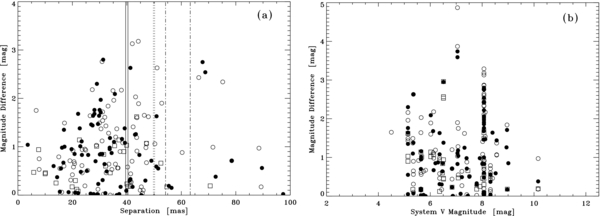
Figure 1. (a) Magnitude difference as a function of separation for the full set of measures described in the text, including those judged not to be of high enough quality to report. A handful of separation measures above 100 mas were present in the sample, but the plot has been truncated to clearly show the behavior at sub-diffraction-limited separations. (b) Magnitude difference as a function of system V magnitude for the same sample. In both plots, the open circles are measures taken with the 550 or 562 nm filter, filled circles are measures in the 698 or 692 nm filter, and squares are measures taken in the 754 or 880 nm filters. In (a), the two solid vertical lines mark the diffraction limit for 550 and 562 nm, the dotted lines mark the same for 692 and 698 nm, and the dot-dashed lines mark 754 and 880 nm.
Download figure:
Standard image High-resolution imageIn Figure 2, we explore the astrometric repeatability of the sample by pairing observations wherever possible, either by using the simultaneous observations in the case of DSSI or sequential observations in pre-DSSI observations. (In the latter case, the second observation was only required to be during the same observing run as the first observation, not directly sequential in time.) Figure 2(a) shows the behavior of the position angle differences between each pair, while Figure 2(b) shows the separation differences. Both are plotted as a function of the average separation obtained. The mean value for the position angle difference is  , while the subset of observation pairs taken in different filters, this is reduced to
  . For the subset of observation pairs taken in different filters and simultaneously, the result is
  . In separation, the average differences for the same three samples are
  mas,
mas,  mas, and
  mas, respectively. Turning now to the standard deviations for these three samples, we obtain σΔθ = 22
 5 ± 20, σΔθ = 131 ± 13, and σΔθ = 93 ± 11 in position angle and σΔρ = 10.4 ± 0.9 mas, σΔρ = 4.3 ± 0.4 mas, and σΔρ = 3.5 ± 0.4 mas. In general, these values appear to indicate that better repeatability is achieved when the observations are obtained simultaneously. There is also basic consistency between the position angle and separation values, as the average separation of the sample is approximately 30 mas and, at that separation, a linear measurement difference of 3.5 mas represents an angle difference of approximately
  , compared with the measured value of ∼9°. The fact that the measured value is slightly larger than the linear prediction is easily explained by the smallest separation systems, where the predicted angle would be much larger than that of the average separation.

Figure 2. Measurement differences between paired observations plotted as a function of average measured separation, ρ. (a) Position angle (θ) differences and (b) separation (ρ) differences. In both plots, filled circles indicate results for paired measures with different filters and the same observation date, open circles are drawn when the two observations did not occur on the same date but during the same run, and squares indicate observations taken on the same date in the same filter. As in Figure 1(a), the vertical lines mark the diffraction limit for the filters used; from left to right these are 550 and 562 nm (solid lines), 698 and 698 nm (dotted lines), and 754 and 880 nm (dot-dashed line).
Download figure:
Standard image High-resolution imageTaking the 3.5 mas figure as the best-case scenario, we note that this figure should be approximately equal to  times the true standard deviation of the sample, since in the subtraction, the sample standard deviation is added in quadrature with itself (assuming Gaussian errors). Furthermore, if the astrometry from the two observations is averaged, then this would decrease the sample standard deviation by another factor of
  . Therefore, the best case of the precision value for paired, averaged astrometry is 3.5/2 = 1.8 mas. This is somewhat higher than what we have recently found for observations above the diffraction limit (1.1 mas in Paper II), but given the more challenging nature of sub-diffraction-limited work, still good enough to be quite useful even at very small separations.
2.2. Astrometric Properties
Of the 222 observations initially identified as of interest for this project, 90 are of objects with orbits in the Sixth Catalog of Visual Binary Star Orbits (Hartkopf et al. 2001b). If we consider only objects with ephemeris separation below the diffraction limit at the time of observation and having published uncertainties in the orbital elements, 66 observations remain. This provides an excellent sample with which to study the measurement accuracy and precision in the sub-diffraction-limited case. We can first study the observed minus ephemeris residuals from the orbits for these measures, treating each measure singly, that is, not pairing any observations, even if two were taken at the same time. This is shown in Figure 3. In calculating the ephemeridal uncertainties δθ and δρ in each case from the published uncertainties in the orbital elements, we find a large range of values. This highlights the fact that the orbits themselves have a range in quality, but if we consider the highest quality orbits as those with δθ ⩽ 120 and δρ ⩽ 5 mas, then we obtain a mean residual of  with standard deviation of σΔθ = 34.0 ± 36. For separation, the results are
  mas with standard deviation of σΔρ = 10.2 ± 1.0 mas. The largest residuals in both cases occur at the smallest ephemeris separations, below ∼20 mas. If only observations above this value are considered, then the mean and standard deviations are
  and σΔθ = 24.8 ± 24 for position angle, and
  mas and σΔρ = 6.6 ± 0.9 mas in separation. The standard deviation values contain both the uncertainty in the ephemeris and the error, both random and systematic, from our measures. Nonetheless, these results indicate that it is unwise to report measures below 20 mas because there is at minimum a systematic overestimate of the separation in these cases. Above this ephemeris separation, on the other hand, there is no evidence for a significant offset in either coordinate.
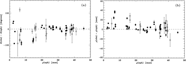
Figure 3. Observed minus ephemeris differences in position angle and separation when comparing the measures presented here with orbital ephemerides of objects having orbital parameters with uncertainties in the Sixth Orbit Catalog of Hartkopf et al. (2001a). Paired observations are treated as two single observations for the purposes of this plot. (a) Position angle residuals and (b) separation residuals. In both plots, filled circles represent the orbits of the highest quality as described in the text, and the error bars are calculated for the observation date based on uncertainties in the orbital parameters appearing in the Sixth Orbit Catalog.
Download figure:
Standard image High-resolution imageNext, we can pair observations and examine the residuals in this case. We consider three types of pairs: (1) pairs where both observations are taken during the same telescope pointing and are in different filters (sequentially if taken before DSSI was completed in 2008 and simultaneously if taken with DSSI), (2) pre-DSSI pairs that are not taken on the same pointing but are from the same run and are in different filters, and (3) observations taken in the same pointing but in the same filter. These residuals are shown in Figure 4, with observation Type 1 drawn as filled circles, observation Type 2 as open circles, and observation Type 3 shown as crosses. The horizontal axis used in these plots is the difference in secondary position between the two observations in arcseconds divided by the mean separation, which represents a dimensionless consistency parameter characterizing the observation pair. The plots demonstrate that requiring consistency between the two colors (if the observation pair is taken in two filters) does help to distinguish between observations affected by systematic error (most likely residual dispersion) and those that are more trustworthy. On the other hand, the one-filter pairs can have a large residual but a small abscissa, indicating that the color information is indeed necessary to make this determination. Note that there will be some duplication in these plots due to cases that can be considered in either Type 2 or Type 3, depending on how the data files for a given run are paired.
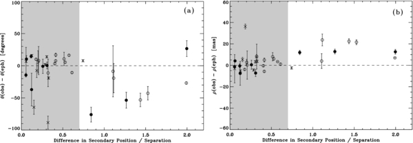
Figure 4. Observed minus ephemeris differences in position angle and separation when comparing the paired measures presented here with orbital ephemerides of objects having orbital parameters with uncertainties in the Sixth Orbit Catalog of Hartkopf et al. (2001a). The astrometry of both observations has been averaged prior to obtaining the residuals. (a) Position angle residuals and (b) separation residuals. In both plots, filled circles represent paired observations at the same observation date and open circles observations with different observation dates but during the same run. Crosses are observation pairs taken in the same filter. The x-axis in both cases is the difference in secondary location between the filters divided by the average observed separation. The gray region marks more consistent observation pairs.
Download figure:
Standard image High-resolution imageFigure 4 suggests that the following simple approach can be used in the analysis of our sub-diffraction-limited observations:
- 1.Wherever possible, an observation should be paired with another taken in a different filter. That is, observation Type 1 defined above is most desirable, followed by observation Type 2. For such observation pairs, calculating the difference in secondary position divided by the average separation and applying the data cut at 0.7 will ensure high data quality without significant systematic error.
- 2.For observations that cannot be paired with another observation in a different filter, one must apply a data cut in observed separation at 20 mas, and not report measures below this value, as these are susceptible to systematic error. Observed separation is essentially a proxy for ephemeris separation in this context, since many observations will not have an orbital prediction. As a consequence, this data cut may not eliminate systematic error completely since the effect is to increase the observed separation (possibly above the limit of 20 mas); however, it is the only observable available for this purpose.
3. RESULTS
Using the above strategy, we construct two final tables, one which consists of unpaired observations (Table 1) and the other which consists of paired observations where the astrometry and observation date (if different between the two observations of the pair) have been averaged (Table 2). The majority of measures in the latter table were taken with DSSI. The format for both tables is the same: (1) the Washington Double Star (WDS) number (Mason et al. 2001a), which also gives the right ascension and declination for the object in 2000.0 coordinates; (2) the Bright Star Catalogue (i.e., Harvard Revised, HR) number, or if none, the Aitken Double Star (ADS) Catalogue number, or if none, the Henry Draper Catalogue (HD) number, or if none, the Durchmusterung (DM) number of the object; (3) the Discoverer Designation; (4) the Hipparcos Catalogue number (ESA 1997); (5) the Besselian date of the observation; (6) the position angle (θ) of the secondary star relative to the primary, with north through east defining the positive sense of θ; (7) the separation of the two stars (ρ), in arcseconds; (8) the magnitude difference (Δm) of the pair (9) center wavelength of the filter used; and (10) width of the filter in nanometers. Position angles have not been precessed from the dates shown and are left as determined by our analysis procedure, even if inconsistent with previous measures in the literature. Determination of the correct quadrant is extremely challenging for many of the data in these tables due to the small separations and the fact that many systems detected have relatively small magnitude differences, as shown in Figure 1(a). This implies that when using these data for orbit determinations, quadrant flips will inevitably be needed at a later stage in some number of cases.
Table 1. Unpaired Double Star Speckle Measures
| WDS | HR, ADS, | Discoverer | HIP | Date | θ | ρ | Δm | λ | Δλ |
|---|---|---|---|---|---|---|---|---|---|
| (α,δ J2000.0) | HD, or DM | Designation | (2000+) | (°) | ('') | (mag) | (nm) | (nm) | |
| 00085 + 3456 | HD 375 | HDS 17 | 689 | 6.5257 | 47.6 | 0.0457 | 0.04 | 550 | 40a |
| 00463 − 0634 | HD 4393 | HDS 101 | 3612 | 8.7019 | 108.5 | 0.0472 | 1.07 | 550 | 40 |
| 00463 − 0634 | HD 4393 | HDS 101 | 3612 | 8.7020 | 100.6 | 0.0503 | 1.06 | 550 | 40 |
| 00507 + 6415 | HR 233 | MCA 2 | 3951 | 4.9750 | 341.5 | 0.0208 | 0.65 | 550 | 40a |
| 00507 + 6415 | HR 233 | MCA 2 | 3951 | 6.5257 | 26.7 | 0.0460 | 0.10 | 550 | 40a |
| 00516 + 4412 | HD 4901 | YR 19Aa,B | ⋅⋅⋅ | 7.8258 | 122.4 | 0.1019 | 0.38 | 550 | 40b |
| 01576 + 4205 | BD+41 379 | YSC 125 | 9121 | 7.8230 | 32.7 | 0.0208 | 0.85 | 698 | 39c |
| 02085 − 0641 | HD 13155 | HDS 284 | 9981 | 4.9724 | 92.5 | 0.2542 | 2.57 | 754 | 44 |
| 02085 − 0641 | HD 13155 | HDS 284 | 9981 | 4.9724 | 92.5 | 0.2624 | 2.53 | 754 | 44 |
| 02128 − 0224 | ADS 1703 | TOK 39Aa,Ab | 10305 | 9.7534 | 171.6 | 0.0229 | 1.01 | 692 | 40 |
| 02169 + 0947 | HD 14068 | OCC 574 | 10634 | 8.0689 | 352.1 | 0.0507 | 0.58 | 698 | 39 |
| 02366 + 1227 | HD 16234 | MCA 7 | 12153 | 7.0094 | 297.9 | 0.0377 | 0.17 | 698 | 39 |
| 02366 + 1227 | HD 16234 | MCA 7 | 12153 | 9.7535 | 168.4 | 0.0564 | 0.15 | 692 | 40 |
| 02424 + 2001 | HD 16811 | BLA 1Aa,Ab | 12640 | 2.7908 | 175.9 | 0.0226 | 1.14 | 754 | 44a |
| 02424 + 2001 | HD 16811 | BLA 1Aa,Ab | 12640 | 7.0094 | 285.2 | 0.0337 | 0.95 | 698 | 39a |
| 03307 − 1926 | HD 21841 | HDS 441 | 16348 | 7.0122 | 171.4 | 0.0525 | 0.66 | 754 | 44 |
| 03307 − 1926 | HD 21841 | HDS 441 | 16348 | 8.6996 | 202.3 | 0.1352 | 0.01 | 698 | 39a |
| 03391 + 5249 | HD 22451 | YSC 127 | 17033 | 8.7024 | 39.2 | 0.0314 | 0.02 | 550 | 40a |
| 06035 + 1941 | HR 2130 | MCA 24 | 28691 | 4.9727 | 243.4 | 0.0389 | 0.90 | 754 | 44a |
| 06035 + 1941 | HR 2130 | MCA 24 | 28691 | 4.9727 | 241.1 | 0.0399 | 1.03 | 754 | 44a |
| 06035 + 1941 | HR 2130 | MCA 24 | 28691 | 8.0691 | 177.5 | 0.0290 | 2.30 | 698 | 39 |
| 08017 + 6019 | HR 3109 | MCA 33 | 39261 | 7.0046 | 345.0 | 0.0355 | 1.02 | 754 | 44a |
| 08017 + 6019 | HR 3109 | MCA 33 | 39261 | 7.0046 | 343.0 | 0.0371 | 1.14 | 754 | 44a |
| 13175 − 0041 | HR 5014 | FIN 350 | 64838 | 7.0105 | 222.2 | 0.0716 | 0.99 | 550 | 40a |
| 13235 + 6248 | HD 116655 | YSC 131 | 65336 | 9.4571 | 45.6 | 0.0380 | 2.17 | 562 | 40a |
| 13598 − 0333 | HR 5258 | HDS 1962 | 68380 | 7.0078 | 353.6 | 0.0559 | 0.96 | 550 | 40a |
| 13598 − 0333 | HR 5258 | HDS 1962 | 68380 | 8.0699 | 238.3 | 0.0394 | 1.08 | 698 | 39a |
| 17217 + 3958 | HR 6469 | MCA 47 | 84949 | 8.4744 | 352.7 | 0.0202 | 0.92 | 550 | 40a |
| 17247 + 3802 | HD 157948 | HSL 1Aa,Ab | 85209 | 6.5250 | 61.9 | 0.0449 | 0.10 | 550 | 40a,d |
| 17247 + 3802 | HD 157948 | HSL 1Aa,Ab | 85209 | 6.5250 | 59.0 | 0.0206 | 0.69 | 550 | 40a,d |
| 17247 + 3802 | HD 157948 | HSL 1Aa,Ac | 85209 | 6.5250 | 235.8 | 0.2143 | 2.33 | 550 | 40 |
| 17247 + 3802 | HD 157948 | HSL 1Aa,Ac | 85209 | 6.5250 | 234.4 | 0.2362 | 2.42 | 550 | 40 |
| 18099 + 0307 | HR 6797 | YSC 132 | 89000 | 8.4666 | 319.6 | 0.0289 | 1.01 | 754 | 44a |
| 18439 − 0649 | HR 7034 | YSC 133 | 91880 | 8.4638 | 170.8 | 0.0344 | 0.87 | 698 | 39a |
| 18582 + 7519 | AC+75 7157 | WOR 26 | 93119 | 7.4236 | 351.2 | 0.0706 | 0.19 | 754 | 44a |
| 18582 + 7519 | AC+75 7157 | WOR 26 | 93119 | 8.4749 | 341.7 | 0.1181 | 0.18 | 550 | 40a |
| 19264 + 4928 | HD 183255 | YSC 134 | 95575 | 8.4639 | 202.3 | 0.0301 | 0.84 | 698 | 39 |
| 19533 + 5731 | HR 7608 | YSC 137 | 97870 | 7.8250 | 28.9 | 0.0352 | 1.96 | 550 | 40a |
| 19533 + 5731 | HR 7608 | YSC 137 | 97870 | 8.4694 | 18.2 | 0.0436 | 1.62 | 754 | 44a |
| 20158 + 2749 | HR 7744 | CHR 94Aa,Ab | 99874 | 7.8196 | 330.7 | 0.0464 | 1.65 | 550 | 40 |
| 20306 + 1349 | HD 195397 | HDS 2932 | 101181 | 7.3225 | 212.6 | 0.0339 | 0.46 | 754 | 44a |
| 20306 + 1349 | HD 195397 | HDS 2932 | 101181 | 7.8196 | 238.8 | 0.0423 | 1.41 | 550 | 40 |
| 20306 + 1349 | HD 195397 | HDS 2932 | 101181 | 8.4612 | 258.8 | 0.0386 | 1.08 | 550 | 40 |
| 23285 + 0926 | HD 221026 | YSC 138 | 115871 | 7.8228 | 204.4 | 0.0337 | 0.98 | 698 | 39a |
| 23347 + 3748 | HD 221757 | YSC 139 | 116360 | 8.7019 | 264.2 | 0.0416 | 0.27 | 550 | 40a |
| 23417 + 4825 | HD 222590 | HDS 3366 | 116895 | 8.6993 | 199.8 | 0.0269 | 1.46 | 698 | 39a |
| 23551 + 2023 | HD 224087 | YSC 140 | 117918 | 7.8228 | 246.8 | 0.0433 | 1.26 | 698 | 39a |
Notes. aQuadrant ambiguous. bThis observation was previously presented in Horch et al. (2010). The data appearing here are the result of a reanalysis using a trinary fit, although the Aa,Ab component was not of high enough quality to include here. cThere is some evidence of a very faint third component in this system with separation of 0.45 arcsec. dQuadrant inconsistent with previous measures in the 4th Interferometric Catalog.
Download table as: ASCIITypeset image
Table 2. Paired Double Star Speckle Measures
| WDS | HR, ADS, | Discoverer | HIP | Date | θ | ρ | Δm | λ | Δλ |
|---|---|---|---|---|---|---|---|---|---|
| (α,δ J2000.0) | HD, or DM | Designation | (2000+) | (°) | ('') | (mag) | (nm) | (nm) | |
| 00085 + 3456 | HD 375 | HDS 17 | 689 | 7.0106 | 185.4 | 0.0547 | 0.88 | 550 | 39 |
| 0.71 | 698 | 39 | |||||||
| 00463 − 0634 | HD 4393 | HDS 101 | 3612 | 10.7172 | 242.2 | 0.0290 | 1.37 | 562 | 40 |
| 1.44 | 692 | 40 | |||||||
| 00507 + 6415 | HR 233 | MCA 2 | 3951 | 3.5332 | 310.0 | 0.0380 | 0.56 | 550 | 39a |
| 1.38 | 698 | 39 | |||||||
| 00507 + 6415 | HR 233 | MCA 2 | 3951 | 7.0106 | 192.8 | 0.0461 | 0.97 | 550 | 39 |
| 2.64 | 698 | 39 | |||||||
| 00516 + 4412 | HD 4901 | YSC 123Aa,Ab | ⋅⋅⋅ | 8.6911 | 356.8 | 0.0165 | 0.71 | 562 | 40 |
| 0.25 | 692 | 40 | |||||||
| 00516 + 4412 | HD 4901 | YSC 123Aa,Ab | ⋅⋅⋅ | 10.0044 | 271.1 | 0.0307 | 0.12 | 562 | 40 |
| 0.04 | 692 | 40 | |||||||
| 00516 + 4412 | HD 4901 | YSC 123Aa,Ab | ⋅⋅⋅ | 10.7144 | 291.5 | 0.0154 | 0.79 | 562 | 40 |
| 0.55 | 692 | 40 | |||||||
| 00516 + 4412 | HD 4901 | YR 19Aa,B | ⋅⋅⋅ | 8.6911 | 125.9 | 0.1004 | 0.50 | 562 | 40b |
| 0.05 | 692 | 40b | |||||||
| 00516 + 4412 | HD 4901 | YR 19Aa,B | ⋅⋅⋅ | 10.0044 | 136.4 | 0.0895 | 0.17 | 562 | 40c |
| 0.56 | 692 | 40c | |||||||
| 00516 + 4412 | HD 4901 | YR 19Aa,B | ⋅⋅⋅ | 10.7144 | 132.9 | 0.0931 | 0.37 | 562 | 40 |
| 0.26 | 692 | 40 | |||||||
| 00541 + 6626 | HD 5110 | YSC 19Aa,Ab | 4239 | 10.7144 | 224.9 | 0.0273 | 1.03 | 562 | 40a |
| 0.83 | 692 | 40 | |||||||
| 00541 + 6626 | HD 5110 | HDS 117Aa,B | 4239 | 3.5332 | 110.6 | 0.8551 | 4.87 | 550 | 40 |
| 3.74 | 698 | 40 | |||||||
| 00541 + 6626 | HD 5110 | HDS 117Aa,B | 4239 | 10.7144 | 108.9 | 0.8759 | 3.87 | 562 | 40 |
| 3.59 | 692 | 40 | |||||||
| 01051 + 1457 | ADS 889 | YSC 124Aa,Ab | 5081 | 10.7116 | 89.4 | 0.0260 | 0.61 | 562 | 40a |
| 0.70 | 692 | 40 | |||||||
| 01057 + 2128 | ADS 899 | YR 6Aa,Ab | 5131 | 7.0052 | 17.2 | 0.0185 | 1.49 | 550 | 39 |
| 0.17 | 754 | 44 | |||||||
| 01057 + 2128 | ADS 899 | YR 6Aa,Ab | 5131 | 10.7116 | 187.8 | 0.0358 | 1.37 | 562 | 40a |
| 1.10 | 692 | 40d | |||||||
| 01101 − 1425 | HD 6978 | HDS 153 | 5475 | 10.0073 | 227.6 | 0.0441 | 0.91 | 562 | 40 |
| 0.83 | 692 | 40 | |||||||
| 02085 − 0641 | HD 13155 | HDS 284 | 9981 | 10.8101 | 99.5 | 0.2437 | 2.95 | 692 | 40e |
| 2.96 | 880 | 50 | |||||||
| 02128 − 0224 | ADS 1703 | TOK 39 Aa,Ab | 10305 | 10.7117 | 149.9 | 0.0374 | 0.56 | 562 | 40 |
| 1.16 | 692 | 40 | |||||||
| 02366 + 1227 | HD 16234 | MCA 7 | 12153 | 1.7616 | 37.4 | 0.0271 | 1.64 | 550 | 40a,d |
| 0.02 | 698 | 40 | |||||||
| 02366 + 1227 | HD 16234 | MCA 7 | 12153 | 10.7175 | 123.1 | 0.0551 | 0.19 | 692 | 40 |
| 0.17 | 880 | 50 | |||||||
| 02424 + 2001 | HD 16811 | BLA 1Aa,Ab | 12640 | 10.7118 | 312.8 | 0.0312 | 0.64 | 562 | 40 |
| 0.03 | 692 | 40 | |||||||
| 03022 − 0630 | 18894 | YSC 126 | 14124 | 10.0101 | 153.2 | 0.0373 | 1.19 | 562 | 40 |
| 0.85 | 692 | 40 | |||||||
| 03391 + 5249 | HD 22451 | YSC 127 | 17033 | 10.7147 | 10.8 | 0.0411 | 0.28 | 562 | 40 |
| 0.30 | 692 | 40 | |||||||
| 03391 + 5249 | HD 22451 | YSC 127 | 17033 | 10.8156 | 9.5 | 0.0408 | 0.33 | 692 | 40a |
| 0.18 | 880 | 50 | |||||||
| 03404 + 2957 | BD+29 590 | HDS 465 | 17151 | 10.8100 | 62.0 | 0.0417 | 0.17 | 692 | 40a |
| 0.18 | 880 | 50d | |||||||
| 03496 + 6318 | HD 23523 | CAR 1 | 17891 | 7.8190 | 61.5 | 0.0463 | 0.67 | 550 | 40 |
| 0.00 | 698 | 40 | |||||||
| 04163 + 3644 | HD 26872 | YSC 128 | 19915 | 10.7202 | 57.2 | 0.0318 | 1.84 | 562 | 40a |
| 1.71 | 692 | 40 | |||||||
| 04256 + 1556 | HR 1391 | FIN 342Aa,Ab | 20661 | 7.8191 | 212.2 | 0.0460 | 0.17 | 550 | 40 |
| 0.30 | 698 | 40 | |||||||
| 05072 − 1924 | HD 33095 | FIN 376 | 23818 | 10.8131 | 237.8 | 0.0320 | 0.64 | 692 | 40a |
| 0.60 | 880 | 50 | |||||||
| 06416 + 3556 | 47703 | YSC 129 | 32040 | 10.8160 | 269.2 | 0.0310 | 0.85 | 692 | 40a |
| 0.84 | 880 | 50 | |||||||
| 07338 + 1324 | HD 60183 | YSC 130 | 36771 | 10.8134 | 119.9 | 0.0151 | 0.98 | 692 | 40a |
| 0.25 | 880 | 50 | |||||||
| 08017 + 6019 | HR 3109 | MCA 33 | 39261 | 7.0059 | 345.5 | 0.0396 | 1.60 | 550 | 39a |
| 1.02 | 754 | 44 | |||||||
| 13175 − 0041 | HR 5014 | FIN 350 | 64838 | 7.3286 | 238.8 | 0.0456 | 0.58 | 550 | 40a |
| 1.63 | 698 | 40 | |||||||
| 13175 − 0041 | HR 5014 | FIN 350 | 64838 | 9.4462 | 320.8 | 0.0318 | 0.46 | 562 | 40a |
| 0.31 | 692 | 40 | |||||||
| 13235 + 6248 | HD 116655 | YSC 131 | 65336 | 10.4647 | 23.7 | 0.0302 | 1.54 | 562 | 40 |
| 1.47 | 692 | 40 | |||||||
| 13317 − 0219 | HD 117635 | HDS 1895 | 65982 | 7.3288 | 315.4 | 0.0455 | 1.62 | 550 | 40 |
| 1.25 | 698 | 40 | |||||||
| 13598 − 0333 | HR 5258 | HDS 1962 | 68380 | 8.4701 | 264.3 | 0.0226 | 0.94 | 550 | 39a |
| 0.12 | 754 | 44 | |||||||
| 14404 + 2159 | HR 5472 | MCA 40 | 71729 | 7.3233 | 63.7 | 0.0471 | 0.98 | 550 | 39 |
| 1.07 | 754 | 44 | |||||||
| 14404 + 2159 | HR 5472 | MCA 40 | 71729 | 8.4620 | 150.6 | 0.0220 | 2.18 | 550 | 40 |
| 0.67 | 698 | 40 | |||||||
| 16229 − 1701 | HD 147473 | CHR 54 | 80240 | 10.4784 | 42.3 | 0.0351 | 0.00 | 562 | 40d |
| 0.00 | 692 | 40 | |||||||
| 17247 + 3802 | HD 157948 | HSL 1Aa,Ab | 85209 | 6.5182 | 222.1 | 0.0358 | 0.53 | 550 | 39a |
| 0.02 | 698 | 39 | |||||||
| 17247 + 3802 | HD 157948 | HSL 1Aa,Ab | 85209 | 6.5182 | 238.2 | 0.0408 | 0.70 | 550 | 39a |
| 0.09 | 698 | 39 | |||||||
| 17247 + 3802 | HD 157948 | HSL 1Aa,Ab | 85209 | 7.3292 | 243.9 | 0.0248 | 0.58 | 550 | 40a,f |
| 0.02 | 698 | 40 | |||||||
| 17247 + 3802 | HD 157948 | HSL 1Aa,Ab | 85209 | 8.4622 | 53.9 | 0.0266 | 1.72 | 550 | 40a |
| 0.04 | 698 | 40d | |||||||
| 17247 + 3802 | HD 157948 | HSL 1Aa,Ab | 85209 | 8.4704 | 60.5 | 0.0228 | 0.19 | 550 | 39 |
| 0.30 | 754 | 44 | |||||||
| 17247 + 3802 | HD 157948 | HSL 1Aa,Ab | 85209 | 8.4704 | 238.1 | 0.0210 | 0.42 | 550 | 39a,f |
| 0.08 | 754 | 44 | |||||||
| 17247 + 3802 | HD 157948 | HSL 1Aa,Ab | 85209 | 10.4732 | 241.8 | 0.0240 | 0.93 | 562 | 40a |
| 0.48 | 692 | 40 | |||||||
| 17247 + 3802 | HD 157948 | HSL 1Aa,Ac | 85209 | 6.5182 | 236.4 | 0.2314 | 2.60 | 550 | 39 |
| 1.86 | 698 | 39 | |||||||
| 17247 + 3802 | HD 157948 | HSL 1Aa,Ac | 85209 | 6.5182 | 236.8 | 0.2560 | 2.86 | 550 | 39 |
| 2.06 | 698 | 39 | |||||||
| 17247 + 3802 | HD 157948 | HSL 1Aa,Ac | 85209 | 7.3292 | 236.1 | 0.2185 | 2.51 | 550 | 40 |
| 2.02 | 698 | 40 | |||||||
| 17247 + 3802 | HD 157948 | HSL 1Aa,Ac | 85209 | 7.4193 | 236.5 | 0.2030 | 3.13 | 550 | 39 |
| 2.42 | 698 | 39 | |||||||
| 17247 + 3802 | HD 157948 | HSL 1Aa,Ac | 85209 | 7.4193 | 236.5 | 0.2056 | 3.29 | 550 | 39 |
| 2.22 | 698 | 39 | |||||||
| 17247 + 3802 | HD 157948 | HSL 1Aa,Ac | 85209 | 8.4622 | 234.0 | 0.1558 | 2.87 | 550 | 40 |
| 1.91 | 698 | 40 | |||||||
| 17247 + 3802 | HD 157948 | HSL 1Aa,Ac | 85209 | 8.4704 | 234.3 | 0.1503 | 2.11 | 550 | 39 |
| 1.49 | 754 | 44 | |||||||
| 17247 + 3802 | HD 157948 | HSL 1Aa,Ac | 85209 | 8.4704 | 232.8 | 0.1489 | 2.64 | 550 | 39 |
| 1.64 | 754 | 44 | |||||||
| 17247 + 3802 | HD 157948 | HSL 1Aa,Ac | 85209 | 9.4466 | 227.6 | 0.0671 | 2.43 | 562 | 40 |
| 2.75 | 692 | 40 | |||||||
| 17247 + 3802 | HD 157948 | HSL 1Aa,Ac | 85209 | 9.4466 | 228.1 | 0.0720 | 2.34 | 562 | 40 |
| 2.54 | 692 | 40 | |||||||
| 17247 + 3802 | HD 157948 | HSL 1Aa,Ac | 85209 | 10.4732 | 28.0 | 0.0311 | 2.76 | 562 | 40a,f |
| 2.80 | 692 | 40 | |||||||
| 18084 + 4407 | HD 166409 | HDS 2554 | 88852 | 3.6337 | 33.1 | 0.0827 | 0.01 | 550 | 39a,d |
| 1.60 | 698 | 39 | |||||||
| 18084 + 4407 | HD 166409 | HDS 2554 | 88852 | 6.5182 | 126.8 | 0.0327 | 1.20 | 550 | 39a |
| 0.23 | 698 | 39 | |||||||
| 18084 + 4407 | HD 166409 | HDS 2554 | 88852 | 7.4248 | 339.7 | 0.0407 | 0.44 | 550 | 39a |
| 0.23 | 754 | 44 | |||||||
| 18582 + 7519 | AC+75 7157 | WOR 26 | 93119 | 7.4195 | 343.5 | 0.0748 | 0.17 | 550 | 39a |
| 0.38 | 698 | 39 | |||||||
| 19264 + 4928 | HD 183255 | YSC 134 | 95575 | 10.4816 | 51.3 | 0.0240 | 0.95 | 562 | 40 |
| 0.83 | 692 | 40 | |||||||
| 19380 + 3354 | BD+33 3529 | YSC 135Aa,Ab | 96576 | 10.4816 | 133.0 | 0.0254 | 0.51 | 562 | 40a |
| 0.50 | 692 | 40 | |||||||
| 19467 + 4421 | HD 187160 | YSC 136 | 97321 | 10.4737 | 322.8 | 0.0336 | 1.28 | 562 | 40 |
| 1.18 | 692 | 40 | |||||||
| 19533 + 5731 | HR 7608 | YSC 137 | 97870 | 10.4816 | 340.7 | 0.0300 | 1.43 | 562 | 40 |
| 1.64 | 692 | 40 | |||||||
| 19533 + 5731 | HR 7608 | YSC 137 | 97870 | 10.4817 | 328.5 | 0.0290 | 1.49 | 562 | 40 |
| 1.76 | 692 | 40 | |||||||
| 20329 + 4154 | HD 195987 | BLA 8 | 101382 | 7.8183 | 295.5 | 0.0062 | 1.75 | 550 | 39a |
| 0.47 | 754 | 44 | |||||||
| 22087 + 4545 | HR 8448 | YSC 15 | 109303 | 10.4819 | 344.6 | 0.0295 | 1.12 | 562 | 40a |
| 1.68 | 692 | 40 | |||||||
| 23049 + 0753 | HD 218055 | YR 31 | 113974 | 7.8214 | 359.5 | 0.0267 | 0.46 | 550 | 40 |
| 1.64 | 698 | 40 | |||||||
| 23347 + 3748 | HD 221757 | YSC 139 | 116360 | 10.7197 | 272.5 | 0.0330 | 0.64 | 562 | 40a |
| 0.49 | 692 | 40 | |||||||
| 23417 + 4825 | HD 222590 | HDS 3366 | 116895 | 10.7198 | 252.8 | 0.0191 | 0.06 | 562 | 40a |
| 1.68 | 692 | 40d |
Notes. aQuadrant ambiguous. bThis observation was previously presented in Paper I. The data presented here are the result of a reanalysis using a trinary fit to include the small separation component YR 123Aa,Ab. cIn the course of reanalyzing this observation to include the small separation component YR 123Aa,Ab, it was noticed that the magnitude differences appearing in Paper II for the two filters shown were reversed. The values appearing here correct that error. dThe observation in this filter had a quadrant inconsistent with the other observation and was flipped prior to averaging the two position angle values. ePossible sub-diffraction-limited component, but the astrometry is not consistent between the two observations. fQuadrant inconsistent with previous measures in the 4th Interferometric Catalog.
A total of 18 objects in these tables have no previous detection in the 4th Catalog of Interferometric Measures of Binary Stars (Hartkopf et al. 2001a); we propose discoverer designations of YSC (Yale-Southern Connecticut) 123-140 here. Thirteen of these objects are known to be spectroscopic binaries from the Geneva–Copenhagen Catalogue or another source, two others are listed as "suspected binaries" in the Hipparcos Catalogue, one has no previous indication of binarity in the literature so far as we are aware (HIP 97870 = HR 7608), and the remaining two are first detections of new small-separation components in known binary systems.
3.1. Astrometric Accuracy and Precision
We study the final astrometric accuracy and precision in the same way as described above for the full set of observations, that is, by comparing to the ephemeris position of those objects with orbits in the Sixth Orbit Catalog. We confine our attention to only those orbits which have published uncertainties for the orbital elements, shown in Table 3. The astrometric properties of the observations in the two final tables are detailed in Table 4 and in Figure 5. In the former, we show the number of measures, average residual (observed minus ephemeris), and standard deviation in both separation and position angle for five subgroups of data: (1) all unpaired observations (i.e., those appearing in Table 1), (2) observations that are paired but which were taken in different telescope pointings, (3) those paired but taken during the same telescope pointing, (4) all paired observations (i.e., those appearing in Table 2), and (5) the paired observations of the objects with the highest quality orbits (with ephemeris uncertainty of less than 5 mas in separation or less than 12° in position angle, respectively. The average residuals of these subsamples show a scatter around 0 of up to ∼2σ in the worst case; nonetheless, the sample sizes are not large here and the unpaired observations as well as the sample of all paired observations do not appear to have values that differ significantly from zero. The standard deviations are larger for the unpaired sample than for the all-paired sample; this is at least partly due to the fact that we have averaged the astrometry in the case of the paired observations. However, error from the ephemerides is also included here.
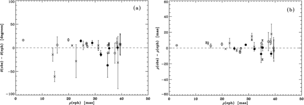
Figure 5. Observed minus ephemeris differences in position angle and separation when comparing the measures presented here with orbital ephemerides of objects having orbital parameters with uncertainties in the Sixth Orbit Catalog of Hartkopf et al. (2001a). Paired observations taken in the same telescope pointing are shown as filled circles, paired observations taken in different pointings are shown as open circles, and unpaired observations are shown as crosses. Paired observations are subject to the data cut diff/sep < 0.7, and unpaired observations subject to observed separation > 0.02 arcsec. (a) Position angle residuals and (b) separation residuals.
Download figure:
Standard image High-resolution imageTable 3. Orbits Used for the Final Measurement Precision Study
| WDS | Discoverer Designation | HIP | Grade | Orbit Reference |
|---|---|---|---|---|
| 00507 + 6415 | MCA 2 | 3951 | 3 | Mason et al. 1997 |
| 01057 + 2128 | YR 6Aa,Ab | 5131 | 3 | Horch et al. 2011 |
| 02366 + 1227 | MCA 7 | 12153 | 2 | Mason 1997 |
| 02424 + 2001 | BLA 1Aa,Ab | 12640 | 2 | Mason 1997 |
| 06416 + 3556 | YSC 129 | 32040 | 9 | Ren & Fu 2010, a |
| 08017 + 6019 | MCA 33 | 39261 | 3 | Balega et al. 2004 |
| 13175 − 0041 | FIN 350 | 64838 | 2 | Hartkopf et al. 1996 |
| 17247 + 3802 | HSL 1Aa,Ab | 85209 | 3 | Horch et al. 2006b |
| 20329 + 4154 | BLA 8 | 101382 | 8 | Torres et al. 2002, b |
| 23347 + 3748 | YSC 139 | 116360 | 9 | Ren & Fu 2010, a |
Notes. aNo measures of these objects appear in the 4th Interferometric Catalog, but an orbit has been obtained by fitting revised Hipparcos intermediate astrometric data. bOnly two successful measures of this object appear in the 4th Interferometric Catalog, but an orbit has been obtained with long baseline optical interferometry.
Download table as: ASCIITypeset image
Table 4. Measurement Precision Results
| Data Group | Observed | Number | Average | Standard | Avg. Eph. | Subtracting |
|---|---|---|---|---|---|---|
| Parameter | of Meas. | Residual | Deviation | Uncertainty | in Quad. | |
| Unpaired observations (Table 1) | ρ | 14 | 3.2 ± 2.3 mas | 8.7 ± 1.6 mas | 5.5 ± 1.4 mas | 6.7 ± 2.4 mas |
| Paired, diff. pointing | ρ | 11 | 2.2 ± 1.4 mas | 4.5 ± 1.0 mas | 3.5 ± 1.4 mas | 2.8 ± 2.4 mas |
| Paired, same pointing | ρ | 6 | −2.0 ± 1.9 mas | 4.6 ± 1.3 mas | 3.8 ± 1.6 mas | 2.6 ± 3.3 mas |
| All paired (Table 2) | ρ | 17 | 0.7 ± 1.2 mas | 4.9 ± 0.8 mas | 3.6 ± 1.0 mas | 3.3 ± 1.6 mas |
| All paired with δρeph < 5 mas | ρ | 14 | 0.8 ± 1.2 mas | 4.4 ± 0.8 mas | 1.8 ± 0.3 mas | 4.0 ± 0.9 mas |
| Unpaired observations (Table 1) | θ | 14 | −68 ± 55 |
206 ± 39 |
155 ± 40 |
136 ± 75 |
| Paired, diff. pointing | θ | 11 | 56 ± 28 |
92 ± 20 |
76 ± 26 |
52 ± 52 |
| Paired, same pointing | θ | 6 | −45 ± 77 |
189 ± 55 |
88 ± 36 |
167 ± 65 |
| All paired (Table 2) | θ | 17 | 20 ± 33 |
138 ± 24 |
80 ± 20 |
112 ± 33 |
| All paired with δθeph < 120 |
θ | 13 | 53 ± 27 |
97 ± 19 |
39 ± 09 |
89 ± 21 |
Download table as: ASCIITypeset image
To obtain an estimate of the true measurement uncertainty, we compute the average ephemeris uncertainty and subtract this in quadrature from the standard deviation, in essence assuming that the measurement errors here and those of the orbital elements are uncorrelated. (Since all of the orbits used here have uncertainties in orbital parameters listed in the Sixth Catalog, we can use these to compute uncertainties in the observables ρ and θ for a desired observation date.) The final values for the measurement uncertainty in separation are 6.7 mas for the observations in Table 1 and 3.3 mas for those in Table 2. The other values in the same (rightmost) column of the table indicate that there is no significant advantage in precision when pairing observations taken on the same telescope pointing (either sequentially for pre-DSSI observations or simultaneously with DSSI) and those taken on different pointings but during the same observing run. This provides the justification for combining all such pairings into Table 2. For the position angle, we find values of 136 for the unpaired observations and 112 for the paired observations. These may be converted into an estimate of the linear measurement uncertainty orthogonal to separation by computing the arctangent and multiplying by the average separation; in doing so, we find that the unpaired observations have value 7.7 mas and the all-paired sample has value 5.8 mas. Finally, since these values are measured orthogonal to the separation and therefore represent independent values, we can average these with those mentioned above to obtain a final linear measurement precision. For unpaired observations (Table 1), the result is 7.2 mas and for the all-paired sample (Table 2) it is 4.6 mas. Recalling that the measures in Table 2 are the average of those obtained in two filters, we would expect the difference in precision to be a factor of  between the two samples; indeed,
  = 5.1 mas, very similar to 4.6 mas. However, it is important to emphasize that the paired observations also represent a sample that includes separations at and below 0.25 of the diffraction limit, while the unpaired sample is limited to somewhat larger separations.
To give a feel for the data used in this study, we show three of the orbits used in the study in Figures 6 and 7. In Figure 6(a), we plot existing and new data for YR 6Aa,Ab together with our own recent orbit determination (Paper II). The new data presented here fall very close to the predicted orbital path, although it should be stated that all data to date has been reported by our group, and a greater diversity of observers would be desirable in order to make certain that no systematic trends exist. Figure 6(b) shows the orbital data of BLA 1Aa,Ab, where the orbit is that of mason (1997). In this case, there is more scatter in the orbital points most likely owing to the contributions of several observers, but again, despite the small scale of the orbit by speckle standards, the data quality of the points presented here is reasonably good.
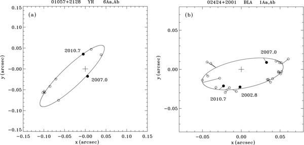
Figure 6. Two examples of objects in Tables 1 and 2 with orbits. (a) The orbit of Horch et al. 2011 for YR 6Aa,Ab = HIP 5131 = HR 310 together with data from the literature and our measures from Table 2. The latter are shown with filled circles. (b) The orbit of mason (1997) for BLA 1Aa,Ab = HIP 12640 = HD 16811 together with our measures from Tables 1 and 2. The latter are shown with filled circles. In both plots, all points are drawn with line segments from the data point to the location of the ephemeris prediction on the orbital path. North is down and east is to the right.
Download figure:
Standard image High-resolution imageIn Figure 7, we show the multiple system HIP 85209 = HD 157948. This is a hierarchical quadruple system, where the widest component (COU 1142) has a separation of approximately 2 arcsec and is not shown. (This component has shown little motion over the last 20 years according to data in 4th Interferometric Catalog.) However, the innermost pair, a spectroscopic binary whose orbit was determined by Latham et al. (1992) and updated by Goldberg et al. (2002), was resolved and measured several times by Horch et al. (2006b) using the Fine Guidance Sensors (FGSs) on the Hubble Space Telescope. The FGS observations also revealed the presence of an intermediate-separation component (HSL 1Aa,Ac) that has been easily monitored with speckle observations at WIYN over the past few years. This component has a number of measures in Tables 1 and 2 and is the most frequently measured component that is well above the diffraction limit, due to our interest in the spectroscopic pair here. The plot of the orbital data shows that HSL 1Aa,Ac has undergone significant orbital motion during this period of time, with rapidly decreasing separation. The data in hand end with the 2010 sub-diffraction-limited measure appearing in Table 2. This measure and the one for the spectroscopic pair of the same observation date were obtained with a triple-star fit to the power spectrum resulting in the two sub-diffraction-limited separations (with the fourth component just off of the chip). It is of course possible to fit the data of HSL 1Aa,Ac to an orbit, and we have done so, obtaining a period of approximately 18 years. However, we feel that it is premature to report the other orbital elements at this stage since the 2010 observation has a quadrant ambiguity that affects the period substantially. In any case, the best approach for this system would be to incorporate all of the data available for the system in a simultaneous orbit fit for both HSL 1Aa,Ac and the inner pair. We hope that the data presented here will encourage other observers to work on this system over the next few years.
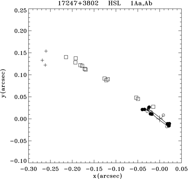
Figure 7. Orbital data for HSL 1 = HIP 85209. For the inner pair, measures appearing the 4th Interferometric Catalog are shown as open circles, and measures from Tables 1 and 2 are shown as filled circles. The orbit plotted is that of Horch et al. (2006b). For the outer component, measures in the 4th Interferometric Catalog are shown as pluses, and the measures from Tables 1 and 2 are shown as squares. North is down and east is to the right.
Download figure:
Standard image High-resolution image3.2. Photometric Accuracy and Precision
Our standard method for estimating the accuracy and precision of our differential photometry in previous papers has been to compare with the space-based magnitude differences appearing in the Hipparcos Catalogue. We have generally considered only speckle observations taken in a filter with properties similar to the Hp filter. However, for objects presented here, there are few that have values listed in the Catalogue, owing to their generally very small separations. Those that were measured by Hipparcos have large uncertainties in ΔHp, typically 0.2 mag or more, much worse than typical for Hipparcos data. Nonetheless, with the sample for which the comparison can be made (12 objects from the paired sample, and 4 from the unpaired), we find observed minus Hipparcos residuals that differ from zero by less than 1σ in both cases, and standard deviations in the 0.4–0.5 magnitude range. However, the mean error of the ΔHp values in both cases is also in the same range. Therefore, we conclude that the measurement error in Δm for sub-diffraction-limited measures is certainly much lower than 0.4 mag, and that there is no evidence at this time that it is significantly larger than what we have previously reported for WIYN speckle data above the diffraction limit, roughly 0.1 mag per observation.
4. ORBIT DETERMINATIONS
4.1. Two Orbit Refinements
In Table 5, we show new orbital elements for two systems for which the observations presented here, together with other relatively recent observations in the 4th Interferometric Catalog, permit modest orbit revisions. To calculate the orbital elements, we have used our own orbit fitting routine, described in MacKnight & Horch (2004). We do not anticipate that these orbits are dramatically better in quality than those published earlier; nonetheless, since they are small-separation systems, the data used span a more complete range in position angle and provide an up-to-date dynamical picture prior to discussing the evolutionary status of the components of these systems.
Table 5. Two Orbit Refinements
| Object | HIP | P | a | i | Ω | T0 | e | ω |
|---|---|---|---|---|---|---|---|---|
| (yr) | (mas) | (°) | (°) | (yr) | (°) | |||
| FIN 350 | 64838 | 9.165 | 80.8 | 55.6 | 201.6 | 2008.39 | 0.632 | 346.8 |
| ±0.010 | ±1.4 | ±2.2 | ±1.2 | ±0.04 | ±0.014 | ±2.3 | ||
| MCA 40 | 71729 | 9.151 | 71.0 | 107.4 | 79.0 | 2003.66 | 0.049 | 265. |
| ±0.041 | ±0.6 | ±0.6 | ±0.6 | ±0.28 | ±0.021 | ±13. |
Download table as: ASCIITypeset image
The first of these binaries is FIN 350(= HIP 64838 = HR 5014), where the previous orbit (which is Grade 2) was computed by Hartkopf et al. (1996). Since that time, several observations have appeared in the literature, including our measures presented here. Our orbit increases both the semi-major axis and the period slightly while decreasing the uncertainties of both substantially. The total mass, when computed with the revised Hipparcos parallax (van Leeuwen 2007), therefore changes from 3.3 ± 3.0 M☉ to 3.4 ± 0.3 M☉. Given that this is an F0V system with at most a small magnitude difference, a total mass of approximately 3.0–3.2 M☉ is expected from the photometry, in excellent agreement with the current orbit. To make the conversion from spectral type to stellar mass, we have used a standard table from the literature (Schmidt-Kaler 1982).
For MCA 40(= HIP 71729 = HD 129132 = HR 5472), the orbit currently listed in the Sixth Catalog is also Grade 2, that of Baize (1989), which we improve upon here at least by estimating uncertainties for the elements. From these we can deduce a total mass of 6.7 ± 1.4 M☉. However, the spectral type in SIMBAD7 is listed as G0V difficult to reconcile with this result. The absolute magnitude derived from an apparent magnitude of 6.23 and revised Hipparcos parallax of 8.60 ± 0.61 mas is +0.83, much too bright for a G-type dwarf pair. (An extinction estimate, though less than 0.1 mag, was included using the NASA/IPAC reddening and extinction map available on the IPAC Web site.8) We suggest therefore that at least the primary is evolved and, given the fact that the magnitude differences observed to date are not terribly large (though with considerable scatter), it may be that both components have left the main sequence. If so, this system could provide quite a sensitive test of stellar evolution theory with more high-quality differential photometry. Graphical representations of our orbits for both FIN 350 and MCA 40 are shown in Figure 8.
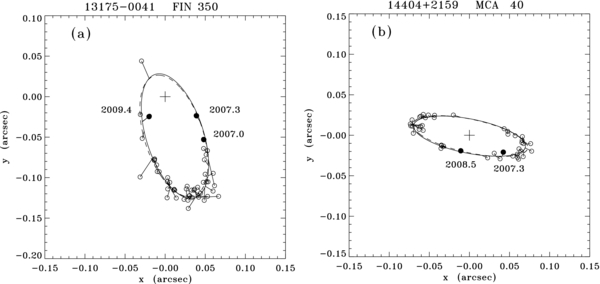
Figure 8. Orbit refinements calculated here for (a) FIN 350 = HIP 64838 and (b) MCA 40 = HIP 71729. Measures appearing the 4th Interferometric Catalog are shown as open circles, and measures from Tables 1 and 2 are shown as filled circles. All points are drawn with line segments from the data point to the location of the ephemeris prediction on the orbital path. The current orbit in the Sixth Catalog is shown as a dashed line. North is down and east is to the right.
Download figure:
Standard image High-resolution image4.2. Three Preliminary Orbits
With the astrometric data in hand from Tables 1 and 2 and in the literature, it is possible to calculate first orbits for three objects, with the caveat that more data will clearly be needed to make the elements definitive. These are shown in Figure 9. However, these orbits, together with photometric and spectroscopic information, permit a useful discussion of the status of these systems at present. The orbital elements we derive are shown in Table 6, and the astrometric data and residuals are shown in Table 7. Here again we have used the fitting routine of MacKnight & Horch (2004).
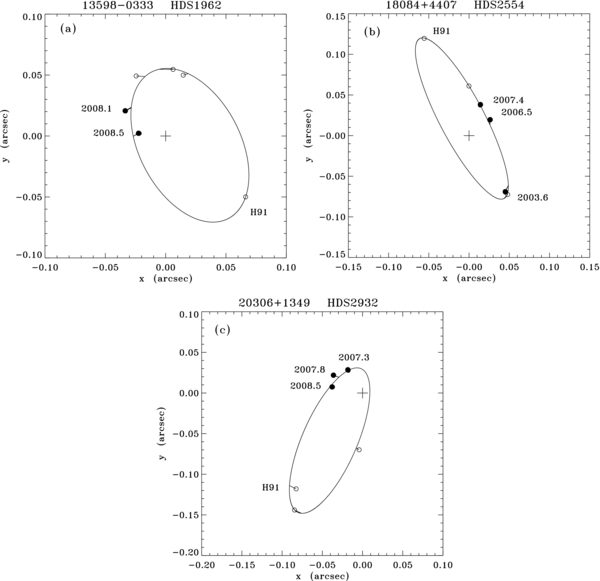
Figure 9. Preliminary orbits for three Hipparcos double stars: (a) HDS 1962 = HIP 68380, (b) HDS 2554 = HIP 88852, and (c) HDS 2932 = HIP 101181. Measures appearing in Tables 1 and 2 are shown as filled circles. The discovery measure of Hipparcos is marked by "H91" in each case.
Download figure:
Standard image High-resolution image
Table 6. Three Preliminary Orbits
| Object | HIP | P | a | i | Ω | T0 | e | ω |
|---|---|---|---|---|---|---|---|---|
| (yr) | (mas) | (°) | (°) | (yr) | (°) | |||
| HDS 1962 | 68380 | 10.7 | 72.7 | 54. | 204. | 2008.29 | 0.413 | 60. |
| ±0.5 | ±5.5 | ±4. | ±4. | ±0.21 | ±0.027 | ±10. | ||
| HDS 2554 | 88852 | 21.6 | 111.8 | 75.3 | 208.3 | 2001.4 | 0.217 | 160. |
| ±0.7 | ±3.1 | ±1.7 | ±1.7 | ±0.7 | ±0.033 | ±12. | ||
| HDS 2932 | 101181 | 26.1 | 122.4 | 66.9 | 170.5 | 2006.12 | 0.829 | 309.5 |
| ±0.6 | ±3.9 | ±1.6 | ±2.0 | ±0.09 | ±0.011 | ±2.5 |
Download table as: ASCIITypeset image
Table 7. Orbital Data and Residuals for the Objects in Table 6
| Object | HIP | Date | θ | ρ | Δθ | Δρ | Reference |
|---|---|---|---|---|---|---|---|
| (Bess. Yr.) | (°) | ('') | (°) | (mas) | |||
| HDS 1962 | 68380 | 1988.163 | ... | <0.038 | [2.2] | [52.5]a | McAlister et al. 1993 |
| 1991.25 | 53. | 0.083 | −0.3 | 1.7 | ESA 1997 | ||
| 2006.1943 | 163.7 | 0.052 | 3.7 | 2.5 | Mason et al. 2009 | ||
| 2007.0078 | 173.6b | 0.0559 | −12.1 | 0.0 | This paper | ||
| 2007.4174 | 206.4 | 0.055 | 7.0 | 3.3 | Horch et al. 2010 | ||
| 2008.0699 | 238.3 | 0.0394 | 7.3 | 2.3 | This paper | ||
| 2008.4701 | 264.3 | 0.0226 | −6.1 | −4.9 | This paper | ||
| HDS 2554 | 88852 | 1991.25 | 205. | 0.132 | 0.1 | −0.3 | ESA 1997 |
| 2002.3229 | 33.5 | 0.087 | 4.2 | −1.7 | Horch et al. 2008 | ||
| 2003.6337 | 33.1 | 0.0827 | −5.5 | 3.6 | This paper | ||
| 2006.5182 | 126.8 | 0.0327 | 9.7 | 2.9 | This paper | ||
| 2007.4248 | 159.7b | 0.0407 | −0.7 | −0.2 | This paper | ||
| 2008.4665 | 180.1 | 0.061 | −1.5 | −2.8 | Horch et al. 2010 | ||
| HDS 2932 | 101181 | 1991.25 | 325. | 0.144 | 3.53 | −1.8 | ESA 1997 |
| 1997.7227 | 329.6 | 0.167 | −3.22 | 5.8 | Mason et al. 1999 | ||
| 1998.7058 | ... | <0.054 | [330.5] | [163.5]a | Mason et al. 2001b | ||
| 2004.8260 | 356.5 | 0.070 | 3.2 | 1.8 | Balega et al. 2007 | ||
| 2007.3225 | 212.6 | 0.0339 | −4.7 | −0.2 | This paper | ||
| 2007.8196 | 238.8 | 0.0423 | 1.8 | 6.8 | This paper | ||
| 2008.4612 | 258.8 | 0.0385 | 1.4 | −2.5 | This paper |
Notes. aThe numbers shown in brackets are the ephemeris values obtained from our orbital elements, therefore indicating the expected position angle and separation for these non-detections. bThe quadrant of this observation has been flipped here relative to that appearing in Table 1 or 2 to make a more sensible sequence in position angle prior to calculating the orbit.
Download table as: ASCIITypeset image
The first of these systems is HDS 1962(= HIP 68380 = HD 122106). Although the latest version of the Geneva–Copenhagen Catalogue (Holmberg et al. 2009) gives the iron abundance of this system as slightly metal-rich, [Fe/H] = +0.13, it does not give a mass ratio. There is a non-detection at 1988.163 by McAlister et al. (1993) for which our orbital elements predict a separation of 52.5 mas. This may be an indication that the data to date produce a period that is slightly too large. If we compute the ephemeris position with P = 10.2 years (1σ lower that the value presented), then the separation is 26 mas, well below the stated limit of the observation of 38 mas. Nonetheless, combining the period and semi-major axis obtained here with the revised Hipparcos parallax of van Leeuwen (2007), the mass sum is 1.6 ± 0.5 M☉. On the other hand, this system has spectral type of F8V in the SIMBAD database, but the absolute magnitude that we calculate from the apparent magnitude, parallax, and extinction (again from the NASA/IPAC online map) is +1.8, too bright by over 1.5 mag to be explained by a pair on the main sequence with that spectral type. The speckle and Hipparcos magnitude differences available in the 4th Interferometric Catalog suggest a value near 1 in V, so perhaps an F7IV–F8V pair comes closer to matching the photometry here. If so, this suggests a mass sum of perhaps 2.5 M☉, somewhat higher than that obtained from the orbit, but within 2σ. If the true value of the period is lower than that of our orbit as the McAlister non-detection suggests, this would of course increase the mass sum, making it more consistent with the 2.5 M☉ value.
The second orbit we present is that of HDS 2554(= HIP 88852 = HD 166409). The Hipparcos data point is in the third quadrant, and subsequent observations have been in the first and second quadrants, thus the position angles available now cover nearly a full orbit since the discovery observation in 1991. This object is slightly below the solar abundance ([Fe/H] = −0.10 according to Holmberg et al. 2009), and once again no mass fraction appears in the Geneva–Copenhagen Catalogue. The system has spectral type F5 in SIMBAD, and the differential photometry that exists at present supports a modest magnitude difference, approximately 0.5 mag. The implied absolute magnitude using the revised Hipparcos parallax is +1.6, which is approximately a magnitude too bright for a main-sequence pair and would seem to suggest that the primary may be slightly evolved. If it is composed of an F(4–5)IV primary and an F(7–8)V secondary, then this implies a total mass in the range of perhaps 2.6–3.0 M☉, whereas the orbital elements in combination with the same parallax value give 3.1 ± 0.5 M☉.
Finally, we have the case of HDS 2932(= HIP 101181 = HD 195397), a system with spectral type F8. Of the three systems discussed here, this is the most metal-poor, with [Fe/H] = −0.17, and the mass fraction in the Geneva– Copenhagen Catalogue is m2/m1 = 0.578 ± 0.037. The magnitude difference appears to be approximately 1, given four measures in the 4th Interferometric Catalog; however, the Hipparcos measure has a large uncertainty and there is significant variation in the three remaining measures. The absolute magnitude derived from the apparent magnitude and revised Hipparcos result is relatively consistent with a main-sequence or near-main-sequence system, so allowing for a sizeable range in secondary spectral type due to the uncertainty in the magnitude difference, perhaps we have an F(6–8)V primary with a G(1–6)V. This implies masses of ∼1.26 ± 0.10 M☉ and 0.96 ± 0.06M☉, so that is a mass ratio of 0.76 ± 0.07. While the mass ratio is larger than that in the Geneva–Copenhagen Catalogue, the total mass agrees quite well with that obtained from our orbital parameters in Table 6 and the parallax, namely 2.0 ± 0.5 M☉. One aspect of the analysis here is difficult to explain: the non-detection by mason et al. in 1998, even though the same group did successfully resolve the system about a year before. We explored orbits which place the secondary below the diffraction limit at their observation date, but this reduces the period significantly, and in view of the photometry and the distance information available, unrealistically. Several of our own measures of this system taken over the past few years were judged to be too poor in quality to report, so more work will be needed to fully understand the nature of this difficulty.
5. CONCLUSIONS
We have analyzed a significant sample of sub-diffraction-limited measures of binary stars taken at the WIYN 3.5 m Telescope over the last several years. These data show that, under certain conditions, it is possible to obtain high-quality measures at separations below 0.25 of the diffraction limit. Sub-diffraction-limited speckle observations are however successful for a smaller range of magnitude differences and only for brighter targets compared with those above the diffraction limit.
It is important to guard against a systematic overestimate of separation in working below the diffraction limit; a reasonably simple and effective way to do this is to take data of the target in two colors and to require consistency in the position of the secondary in both observations. One may also then average the astrometry obtained to reduce random error. Following this strategy leads to results that show no evidence of systematic error and have repeatability of approximately 2 mas. Overall measurement precision for the sample presented here is somewhat higher, approximately 3.3–4.0 mas, but may be attributed to the use of different instrumentation and observing conditions over the years. If two observations in different filters are not available, we find that it is unwise to report separations below approximately 0.5 of the diffraction limit since the systematic overestimate in separation which is most prominent at the smallest separations. We report 47 measures of this type where the linear measurement uncertainty is estimated to be approximately 7 mas.
Modest orbit revisions for two systems are reported; the uncertainties for the orbital elements reported here are small enough to permit a brief report on the evolutionary status of these systems. FIN 350 appears to consist of a late-F + early-G main-sequence system, whereas the data of MCA 40 on balance support an evolved primary and possibly an evolved secondary. New orbits are reported for three Hipparcos double stars. A combination of the orbital information and photometry results in a sensible picture for main-sequence components for HDS 2932, while HDS 1962 and HDS 2554 may have primary stars that have evolved off of the main sequence.
We thank the Kepler Science Office located at the NASA Ames Research Center for providing partial financial support for the upgraded DSSI instrument. It is also a pleasure to thank all of the outstanding staff at WIYN for their assistance and support over the years. This work was funded by NSF Grant AST-0908125. It made use of the Washington Double Star Catalog maintained at the U.S. Naval Observatory and the SIMBAD database, operated at CDS, Strasbourg, France.
Footnotes
- *
The WIYN Observatory is a joint facility of the University of Wisconsin-Madison, Indiana University, Yale University, and the National Optical Astronomy Observatories.
- 7
- 8