


ABSTRACT
The results of 497 speckle observations of Hipparcos stars and selected other targets are presented. Of these, 367 were resolved into components and 130 were unresolved. The data were obtained using the Differential Speckle Survey Instrument at the WIYN 3.5 m Telescope. (The WIYN Observatory is a joint facility of the University of Wisconsin-Madison, Indiana University, Yale University, and the National Optical Astronomy Observatories.) Since the first paper in this series, the instrument has been upgraded so that it now uses two electron-multiplying CCD cameras. The measurement precision obtained when comparing to ephemeris positions of binaries with very well known orbits is approximately 1–2 mas in separation and better than 0 6 in position angle. Differential photometry is found to be in very good agreement with Hipparcos measures in cases where the comparison is most relevant. We derive preliminary orbits for two systems.
Export citation and abstract BibTeX RIS
1. INTRODUCTION
The Differential Speckle Survey Instrument (DSSI), first described in Horch et al. (2009b, hereafter Paper I), has been in regular use at the WIYN Telescope at Kitt Peak since its completion in 2008 September. The instrument is a dual-channel speckle imaging system that uses a dichroic element to send light below a given wavelength to one imaging detector and light above that wavelength to a second identical detector. Thus, the system can take speckle patterns simultaneously in two colors. As discussed in Paper I, this offers three main advantages over single-detector speckle observations. (1) Twice as many frames are detected per unit time, doubling the telescope efficiency, or equivalently, increasing the signal-to-noise ratio for astrometric measurement for a given observation time, since the astrometry should not vary with wavelength. (2) Color information of the components of binary star systems is obtained in a single observation. This can be especially important in rapidly identifying interesting targets in large surveys of binaries, as we are conducting at WIYN. (3) The simultaneous information in two colors gives greater leverage on any residual atmospheric dispersion that may be present in an observation, allowing reliable differential astrometry of binaries to be obtained below the diffraction limit of the telescope, as discussed in Horch et al. (2006).
DSSI was originally designed to use two large-format CCDs as the image capture devices in both channels, and in fact the results in Paper I were obtained with our two Princeton Instruments PIXIS 2048B CCD cameras. The DSSI optics have the ability to quickly move a star image around on the image plane of these detectors using two galvanometric scanning mirrors. This permits many speckle patterns to be collected over the full area of the chip prior to full-frame readout. However, electron-multiplying CCDs (EMCCDs) have recently been shown to be very capable devices for speckle imaging (see, e.g., Tokovinin & Cantarutti 2008; Tokovinin et al. 2010; Horch et al. 2009a; Maksimov et al. 2009; Docobo et al. 2010). For this reason, we have obtained two Andor iXon 897 EMCCDs to use with the DSSI optics package. These devices have a much smaller format than the PIXIS cameras (512 × 512 versus 2048 × 2048 pixels), but have comparable quantum efficiency and read out extremely quickly. This removes the need to change the position of the galvanometric scanning mirrors when taking speckle observations. Furthermore, the electron-multiplying capability of the detectors yields effective read noise of much less than one electron when a high gain is used.
Operating DSSI in the dual-EMCCD mode has significantly improved the typical signal-to-noise ratio in speckle observations of fainter targets, as well as the limiting magnitude of the system for diffraction-limited imaging. As we will show here, the arrangement also appears to deliver extremely good differential photometry of binaries. The combination of the limiting magnitude, astrometric and photometric precision, and sub-diffraction-limited capabilities makes DSSI an ideal system for surveying binaries within 200 pc of the solar system. At that distance, DSSI should be capable of obtaining astrometry for relatively bright systems with separations as small as 2–4 AU. In addition, high-resolution ground-based imaging is currently needed for the Kepler and CoRoT missions as one method to minimize false positives in the data stream for exoplanet detection. The DSSI system is currently taking data for both missions; for more information on the role of ground-based observing, including speckle imaging, in the Kepler mission, see, e.g., Borucki et al. (2010) or S. B. Howell et al. (2011, in preparation).
The results presented in the current paper represent the first major group of observations obtained with the dual-EMCCD arrangement. The focus here is our "standard" speckle analysis; that is, we report results where separations are above the diffraction limit of the telescope in both filters and high-quality non-detections where no evidence of a companion is seen to the diffraction limit in both filters. The objects observed are mainly binaries or suspected binaries that appear in the Hipparcos Catalogue (ESA 1997), but also include a handful of fainter sources to demonstrate detector capabilities. A subsequent paper in this series will present sub-diffraction-limited measures.
2. OBSERVATIONS AND DATA REDUCTION
The observations presented here come from two observing runs using the WIYN Telescope at Kitt Peak, 2010 January 2–4 and June 18–25. Only about half of the observing time during these runs was used for the observations discussed here; the remainder of the time was used for support observations of the Kepler and CoRoT missions. Weather during these runs was generally very good, although the seeing did vary considerably, from approximately 0.5 arcsec to 1.4 arcsec. The two EMCCDs were mounted to the two detector ports on the DSSI optics package as shown in Figure 1 of Paper I; we will refer to these ports as the "side" and "back" ports in the following discussion.
2.1. Pixel Scale and Orientation
Our method for measuring the pixel scale and orientation relative to celestial coordinates is essentially the same as described in Paper I. Briefly, we continue to use a slit mask that we can mount to the tertiary mirror baffle support structure in order to obtain a precise measurement of the pixel scale. When the mask is on the telescope, we take a speckle observation of a bright unresolved star. The slits of the mask (which are in the converging beam but may be effectively mapped back to the aperture plane) give rise to a sequence of linear features in the power spectrum of the speckle observation, with spacing directly related to the spacing of slit pairs on the mask. When combined with the telescope focal length, mounting surface position relative to the image plane, and the wavelength of the observation, the features can be used to provide the scale. Horch et al. (1999) provide more detailed information on this method.
We have found it important to rotate the Nasmyth port of the telescope to various angles during our mask calibrations in order to fully map out the dependence of the pixel scale on position angle that was discussed in Paper I. This is due to a small surface misalignment within the instrument and is visible in the back port of the DSSI optics package. We have again used the model of a tilted surface to calibrate and remove this effect in that channel; no misalignment was detected in the side port of the instrument. Another important consideration in the determination of our final scale values for this paper is the use of calibration stars with a wide variety of color; for the two runs discussed here, four sequences of mask files were taken, two in January and two in June, where the stars chosen ranged in spectral type from B6III to K3Iab. The color of the star changes the effective wavelength of the observation slightly, so that without a range of color, a systematic error in the pixel scale can result. Based on our mask results, we find that the side port has a scale of 21.766 ± 0.028 mas pixel−1. The value for the back port is similar, but varies slightly with position angle due to the surface misalignment. It nonetheless has a similar percentage error to that of the side port, i.e., ∼0.13%. Since the astrometry presented in the next section is the average of both channels, we suggest that the uncertainty due to the scale calibration is 0.13% %.
%.
We use sequences of short exposure (1 s) images of reasonably bright targets to establish the detector orientation. Between two successive exposures, the telescope is offset in a given direction by a small amount (typically 5 arcsec). By determining the centroid of the star in each of these frames and noting the change between exposures, it is possible to determine both the scale and the orientation, although we do not use the scale values in general because the mask results are typically of much higher precision. (Nonetheless, there were no major discrepancies between the two methods for the data presented here.) Offset images are generally taken each night and the results averaged. We did not find any significant change between the January and June runs, so that the final numbers used were the average values of both runs. The position angle offset of celestial coordinates relative to the pixel axes in the side port of the instrument was −538 ± 028, while in the back port, the figure obtained was +515 ± 018. Since our final position angles discussed in the next section are the average of both channels, we estimate that the uncertainty due to our offset measurements may be obtained by adding these two results in quadrature and dividing by two, yielding an orientation uncertainty of ∼017.
2.2. Reduction Method
Our observing routine and reduction method also remain the same as discussed in Paper I. In all of the work presented here, the side port of DSSI was fitted with the 692 nm filter, the back port was fitted with the 562 nm filter, and our red–green dichroic was used. The filter transmission curves of these optics appear in Paper I; the full width at half-maximum of the transmission is 40 nm for both filters. Insofar as it is possible, we try to group our targets together on the sky and observe them in sequence, together with a bright point source calibrator. Unlike the results discussed in Paper I, however, the galvanometer mirrors were held stationary during the observation since the EMCCDs were read out fast enough to maintain good speckle coherence. The typical observation is a sequence of 1000 speckle 128 × 128 pixel subframes centered on the object, with a frame-integration time of 40 ms. Other frame times from 30 to 60 ms were tried, but 40 ms appears to give the highest signal-to-noise ratio for typical observing conditions at WIYN.
Our reduction method continues to be Fourier based, where we compute the average spatial frequency power spectrum for each observation, deconvolve the speckle transfer function by dividing by the power spectrum of the point source, and then compute a weighted least-squares fit of a fringe pattern to a masked version of the resulting function. (The mask sets to zero pixels in the Fourier plane that have low signal-to-noise ratio and low-frequency values judged to be in the seeing disk.) In order to determine the quadrant of the companion star, we compute a reconstructed image via bispectral analysis (e.g., Lohmann et al. 1983).
2.3. Detection Capabilities
With the electron-multiplying gain function enabled, individual photons striking the EMCCD usually generate a signal large enough to clearly see above the read noise. Thus, the device has extremely low effective read noise while maintaining quantum efficiency above 90% through most of the visible spectrum. Although the dynamic range of the device is small in this configuration, the necessity to take short frames in speckle imaging renders this deficiency insignificant. The result is that the limiting magnitude of speckle observations is much fainter than with either low-noise CCDs, which suffer in comparison due to a higher read noise, or microchannel-plate-based devices such as intensified-CCDs (ICCDs), which typically have lower quantum efficiencies.
Tokovinin and his collaborators have made early and extremely effective use of EMCCDs in speckle observations (Tokovinin & Cantarutti 2008; Tokovinin et al. 2010). These papers have clearly shown the potential of these new devices in speckle imaging, leading to their acquisition by both our team and the speckle collaboration working at the Special Astrophysical Observatory 6 m Telescope (e.g., Docobo et al. 2010), among others. In our case, making the change to EMCCDs has been the deciding factor in the use of DSSI in the substantial ground-based follow-up work for Kepler and CoRoT, as the deeper limiting magnitude has made their targets accessible for the first time using speckle imaging at WIYN. While that theme will be developed further in a future paper that details those observations (S. B. Howell et al. 2011, in preparation), it is appropriate here to make a brief study of the detection capability for binary star work in general.
Figure 1(a) shows the magnitude difference obtained as a function of separation for all objects successfully resolved during the January and June runs (and tabulated in the next section). Figure 1(b) shows the same magnitude differences, but plotted as a function of V magnitude of the object. Both figures look very similar to diagrams of this nature that we have previously constructed (see, e.g., Figure 1 of Horch et al. 2010). For example, when plotted against separation, systems with a magnitude difference as large as approximately 5 can be detected through a wide range of separation, with decreasing sensitivity at small separations (<0.2 arcsec), down to a maximum Δm of approximately 3.5 at the diffraction limit. When plotted against V magnitude, systems with magnitude differences as large as 5 are detected at least as faint V = 10, with an apparent decrease as the V magnitude becomes fainter. However, most of the targets observed here are drawn from the Hipparcos Catalogue (ESA 1997), and this downturn is dominated by the apparent-magnitude distribution of those stars, few of which are fainter than magnitude 12. Furthermore, while nothing fainter than a V magnitude of 14 had been successfully detected at WIYN with our previous imaging detectors, Figure 1(b) shows two objects beyond that limit, namely WDS 20367+4021 = NML 2AB = WR 147 (V = 14.9) and WDS 14125+1636 = WSI 117 = LP 439-387 (V = 15.7). It is worth stating that these magnitudes appear to be somewhat uncertain; Niemela et al. (1998) quote magnitudes of the components of NML 2AB as 13.86 and 16.02 based on Hubble Space Telescope Wide Field Planetary Camera 2 images and therefore a system magnitude of 13.72. On the other hand, the Washington Double Star (WDS) Catalog has magnitudes of 15.0 and 17.2, resulting in a system magnitude of 14.87. The latter agrees well with what appears in the SIMBAD database,7 namely 14.89. In the case of WSI 117, while both the SIMBAD database and the WDS agree on a system magnitude of approximately 15.7, the count rate obtained during our observations was somewhat higher than what would be expected for a star of that magnitude (though our astrometry agrees well with that appearing in the WDS, up to a quadrant flip of the secondary).
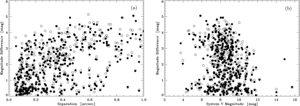
Figure 1. (a) Magnitude difference as a function of separation for the measures listed in Table 1. While a handful of separation measures above 1 arcsec appear there, the plot has been truncated to clearly show the behavior at subarcsecond separations. (b) Magnitude difference as a function of system V magnitude for the measures listed in Table 1. In both plots, the open circles are measures taken with the 562 nm filter and filled circles are measures in the 692 nm filter.
Download figure:
Standard image High-resolution imageTo demonstrate the data quality for faint targets, we show our standard reconstructed images for WSI 117 and NML 2AB in Figure 2, both in the 562 nm and the 692 nm filters. Comparing the images for WSI 117, the secondary appears brighter relative to the primary star in the 562 nm filter, indicating that the companion is bluer than the primary. On the other hand, for NML 2AB, the secondary is detected only in the 692 nm image, with a magnitude difference of over 2.0. This indicates that the companion is almost certainly much redder than the primary. (The 5σ detection limit at the relevant separation as defined in Section 3.3 for the 562 nm observation is approximately 4.5 mag.) The four images together indicate that, even at magnitudes fainter than 14, relatively good image quality can be obtained. Despite some uncertainty in the magnitudes of these objects, we conclude that the detection of companions is probably possible to at least 16th magnitude and possibly fainter, under good observing conditions.

Figure 2. Reconstructed images of faint targets. (a) WSI 117 = LP439-387 in the 562 nm filter. (b) WSI 117 = LP439-387 in the 692 nm filter. (c) NML 2AB = WR 147 in the 562 nm filter. (d) NML 2AB = WR 147 in the 692 nm filter.
Download figure:
Standard image High-resolution image3. RESULTS
Our main body of results is presented in Tables 1 and 2. Table 1 contains the observations where the target was successfully resolved into two or more stars, and Table 2 contains the non-detections. The columns in Table 1 are as follows: (1) the WDS number (Mason et al. 2001b), which also gives the right ascension and declination for the object in 2000.0 coordinates; (2) the Bright Star Catalogue (i.e., Harvard Revised, HR) number, or if none the Aitken Double Star (ADS) Catalogue number, or if none, the Henry Draper (HD) Catalogue number, or if none the Durchmusterung (DM) number of the object, or if none the Gliese-Jareiß Catalogue number; (3) the Discoverer Designation; (4) the Hipparcos Catalogue number; (5) the Besselian date of the observation; (6) the position angle (θ) of the secondary star relative to the primary, with north through east defining the positive sense of θ; (7) the separation of the two stars (ρ), in arcseconds; (8) the magnitude difference (Δm) of the pair in the 562 nm filter; and (9) the magnitude difference of the pair in the 692 nm filter. Position angle and separation measures shown are the values obtained by averaging the results from both channels of the instrument, and position angles have not been precessed from the dates shown. Forty-five objects in Table 1 have no previous detection in the 4th Catalogue of Interferometric Measures of Binary Stars (Hartkopf et al. 2001b); we propose discoverer designations of Yale-Southern Connecticut (YSC) 78–122 here.
Table 1. Double Star Speckle Measures with DSSI
| WDS | HR,ADS | Discoverer | HIP | Date | θ | ρ | Δm | Δm |
|---|---|---|---|---|---|---|---|---|
| (α,δ J2000.0) | HD or DM | Designation | (2000+) | (°) | ('') | (562 nm) | (692 nm) | |
| 00031+5228 | HD 225064 | HDS 3 | 250 | 10.0072 | 333.5 | 0.3284 | 2.88 | 3.03 |
| 00121+5337 | ADS 148 | BU 1026AB | 981 | 10.0072 | 312.6 | 0.3392 | 1.19 | 1.03 |
| 00132+2023 | BD+19 20 | HDS 29 | 1055 | 10.0099 | 165.6 | 0.7307 | 1.78 | 1.58 |
| 00145+1638 | HD 997 | YSC 78 | 1156 | 10.0099 | 44.6 | 0.6335 | 3.78 | 3.28 |
| 00182+5225 | HD 1384 | YSC 79 | 1460 | 10.0072 | 314.0 | 0.3392 | 3.43 | 3.49 |
| 00246+1659 | HD 2020 | YSC 80 | 1946 | 10.0099 | 208.8 | 0.9026 | 4.17 | 3.64 |
| 00260+1905 | HD 2174 | HDS 59 | 2048 | 10.0099 | 263.0 | 0.8275 | 2.61 | 2.30 |
| 00310+5015 | HD 2712 | HDS 68 | 2437 | 10.0072 | 356.1 | 0.4246 | 2.45 | 2.63 |
| 00317+1929 | HD 2815 | HDS 70 | 2502 | 10.0099 | 66.4 | 0.3040 | 2.00 | 2.23 |
| 00321+5000 | BD+49 116 | COU 2151 | 2528 | 10.0072 | 98.8 | 0.1526 | 1.35 | 1.20 |
| 00324+2147 | HD 2891 | HDS 72 | 2549 | 10.0099 | 34.0 | 0.2048 | 0.87 | 0.87 |
Notes. aQuadrant ambiguous. bIn both filters, the quadrant obtained appears to be inconsistent with previous measures in the 4th Interferometric Catalog. However, it is left as measured here pending future determinations. cQuadrant is inconsistent with previous measures in the 4th Interferometric Catalog in the filter marked. The position angle has been changed prior to averaging with the other observation. dTwo 1000-frame observations were co-added to obtain these results. eThree 1000-frame observations were co-added to obtain these results.
Only a portion of this table is shown here to demonstrate its form and content. Machine-readable and Virtual Observatory (VO) versions of the full table are available.
Download table as: Machine-readable (MRT)Virtual Observatory (VOT)Typeset image
Table 2. High-quality Non-detections and 5σ Detection Limits
| (α,δ J2000.0) | HIP | Date | 5σ Det. Lim. | 5σ Det. Lim. | Notes |
|---|---|---|---|---|---|
| (WDS Format) | (2000+) | (562 nm) | (692 nm) | ||
| 00093+1732 | 759 | 10.0099 | 4.72 | 4.16 | G-C spectroscopic binary |
| 00174+1852 | 1389 | 10.0099 | 4.06 | 3.91 | HDS 39; ρ>1'', perhaps off chip? |
| 00393+4156 | 3091 | 10.0044 | 4.43 | 4.46 | Hipparcos suspected double |
| 00495+4404 | 3857 | 10.0044 | 4.96 | 4.01 | HDS 109; previously resolved, below diff. lim.? |
| 00551+4841 | 4298 | 10.0045 | 4.66 | 4.24 | Hipparcos suspected double |
| 00552+2433 | 4317 | 10.0045 | 4.31 | 4.35 | Hipparcos suspected double |
| 01234−1756 | 6487 | 10.0045 | 3.26 | 3.74 | Hipparcos suspected double |
| 01245+2202 | 6577 | 10.0045 | 4.38 | 3.76 | G-C spectroscopic binary |
| 01291+2143 | 6917 | 10.0046 | 4.68 | 4.22 | HO 9A, G-C spectroscopic binary |
| 01308+2311 | 7048 | 10.0046 | 4.32 | 3.86 | HDS 197; also not detected by Mason et al. (1999) |
| 01380+0946 | 7604 | 10.0046 | 4.37 | 4.02 | G-C spectroscopic binary |
| 02110−0155 | 10188 | 10.0046 | 3.35 | 3.65 | Hipparcos suspected double |
| 02128−0224 | 10305 | 10.0046 | 4.25 | 4.46 | TOK 39Aa,Ab, G-C spectroscopic binary |
| 02150−2332 | 10474 | 10.0073 | 3.22 | 4.21 | G-C spectroscopic binary |
| 02176+5801 | 10690 | 10.0074 | 3.54 | 3.23 | Hipparcos suspected double |
| 02243+3950 | 11206 | 10.0074 | 4.54 | 3.55 | HDS 312; previously resolved, below diff. lim.? |
| 02538−0210 | 13497 | 10.0101 | 3.58 | 3.98 | Hipparcos suspected double |
| 03008−0253 | 14040 | 10.0101 | 4.34 | 4.85 | Hipparcos suspected double |
| 03019+1314 | 14111 | 10.0047 | 4.04 | 3.14 | Hipparcos suspected double |
| 03052+3850 | 14354 | 10.0047 | 4.12 | 3.33 | Hipparcos suspected double |
| 03149+1226 | 15117 | 10.0048 | 3.94 | 3.73 | Hipparcos suspected double |
| 03336−0725 | 16596 | 10.0101 | 4.58 | 4.43 | G-C spectroscopic binary |
| 03390+0048 | 17024 | 10.0075 | 4.34 | 4.20 | Hipparcos suspected double |
| 07395+4758 | 37299 | 10.0052 | 4.47 | 4.01 | Hipparcos suspected double |
| 08037+3621 | 39433 | 10.0052 | 4.09 | 3.55 | Hipparcos suspected double |
| 08117+3227 | 40118 | 10.0053 | 3.72 | 3.78 | STT 564A, thick disk candidate |
| 08478+6613 | 43185 | 10.0108 | 3.54 | 3.07 | G-C spectroscopic binary |
| 09025+6738 | 44390 | 10.0108 | 4.42 | 4.35 | Hipparcos suspected double |
| 09038+3845 | 44481 | 10.0054 | 4.45 | 4.41 | Hipparcos suspected double |
| 09202+6501 | 45794 | 10.0108 | 4.17 | 4.46 | G-C spectroscopic binary |
| 09321+6242 | 46794 | 10.0108 | 3.77 | 3.76 | Hipparcos suspected double |
| 09391+5220 | 47376 | 10.0054 | 4.23 | 3.49 | G-C spectroscopic binary |
| 10253+0847 | 51008 | 10.0082 | 5.18 | 4.26 | Hipparcos suspected double |
| 10450+4023 | 52571 | 10.0110 | 4.41 | 4.29 | Hipparcos suspected double |
| 10490+4356 | 52881 | 10.0110 | 4.88 | 4.36 | G-C spectroscopic binary |
| 11017+3641 | 53903 | 10.0111 | 4.23 | 3.87 | HDS 1574; previously resolved, below diff. lim.? |
| 11082+3627 | 54428 | 10.0056 | 3.99 | 3.35 | G-C spectroscopic binary |
| 11084+7158 | 54442 | 10.0084 | 4.36 | 4.07 | G-C spectroscopic binary |
| 11093+3619 | 54522 | 10.0111 | 4.42 | 3.49 | Hipparcos suspected double |
| 11131−1715 | 54799 | 10.0083 | 3.00 | 4.54 | Hipparcos suspected double |
| 11243+6503 | 55662 | 10.0084 | 3.98 | 3.96 | G-C spectroscopic binary |
| 11331+3919 | 56352 | 10.0056 | 3.35 | 3.10 | Hipparcos suspected double |
| 11514+1148 | 57821 | 10.0112 | 4.82 | 4.03 | HDS 1672; previously resolved, below diff. lim.? |
| 12087+2242 | 59219 | 10.0112 | 4.29 | 3.31 | Hipparcos suspected double |
| 12178+2503 | 59952 | 10.0112 | 4.50 | 3.84 | G-C spectroscopic binary |
| 12293+4902 | 60931 | 10.0084 | 3.80 | 3.28 | Hipparcos suspected double |
| 12330+2643 | 61243 | 10.0112 | 3.31 | 3.42 | Hipparcos suspected double |
| 12451+4526 | 62223 | 10.0057 | 4.57 | 4.06 | Hipparcos suspected double |
| 12491+4323 | 62559 | 10.0084 | 4.02 | 3.06 | Hipparcos suspected double |
| 13040+1114 | 63752 | 10.0058 | 3.46 | 4.40 | Hipparcos suspected double |
| 13086+5049 | 64128 | 10.0113 | 3.47 | 3.65 | Hipparcos suspected double |
| 13130+5049 | 64481 | 10.0113 | 3.21 | 3.20 | Hipparcos suspected double |
| 13212+3751 | 65159 | 10.4701 | 5.12 | 5.05 | G-C spectroscopic binary |
| 13220+0245 | 65225 | 10.0085 | 4.42 | 4.72 | Hipparcos suspected double |
| 13277+0352 | 65660 | 10.0085 | 3.01 | 3.06 | Hipparcos suspected double |
| 13298+4034 | 65844 | 10.4619 | 4.71 | 4.89 | Hipparcos suspected double |
| 13299+3431 | 65853 | 10.4619 | 5.28 | 4.86 | Hipparcos suspected double |
| 13467+2542 | 67239 | 10.0085 | 4.66 | 4.05 | G-C spectroscopic binary |
| 13518+3427 | 67665 | 10.4619 | 5.64 | 3.76 | Hipparcos suspected double |
| 13496+1301 | 67470 | 10.0113 | 4.69 | 4.01 | G-C spectroscopic binary |
| 14005+3750 | 68428 | 10.4619 | 3.61 | 4.22 | Hipparcos suspected double |
| 14104+2506 | 69226 | 10.4811 | 5.22 | 5.46 | ISO 14, G-C spectroscopic binary |
| 14121+6926 | 69373 | 10.4648 | 4.20 | 4.64 | Hipparcos suspected double |
| 14129+0951 | 69424 | 10.4674 | 4.00 | 4.84 | Hipparcos suspected double |
| 14149+0320 | 69614 | 10.4757 | 4.66 | 5.30 | Hipparcos suspected double |
| 14177+0344 | 69851 | 10.4757 | 4.84 | 5.16 | G-C spectroscopic binary |
| 14230+3901 | 70297 | 10.4619 | 3.50 | 3.83 | Hipparcos suspected double |
| 14238+0053 | 70364 | 10.4757 | 3.89 | 4.61 | Hipparcos suspected double |
| 14242+2542 | 70401 | 10.4812 | 5.06 | 4.90 | Hipparcos suspected double |
| 14253+3645 | 70502 | 10.4619 | 3.04 | 3.48 | Hipparcos suspected double |
| 14364+5116 | 71431 | 10.4620 | 4.73 | 5.36 | G-C spectroscopic binary |
| 14431−0539 | 71957 | 10.4757 | 4.06 | 4.70 | G-C spectroscopic binary |
| 14471+1820 | 72303 | 10.4674 | 3.98 | 4.15 | G-C spectroscopic binary |
| 14493+4950 | 72486 | 10.4675 | 4.54 | 4.27 | HDS 2091, ρ>1'' |
| 14529+4828 | 72803 | 10.4811 | 3.39 | 4.33 | LEP 70A, thick disk candidate |
| 15009+4526 | 73470 | 10.4811 | 3.40 | 4.19 | HDS 2118; ρ>1 7, off chip 7, off chip |
| 15114+4842 | 74320 | 10.4620 | 4.36 | 4.76 | G-C spectroscopic binary |
| 15118+6151 | 74370 | 10.4702 | 3.87 | 4.79 | STF 1927A, thick disk candidate |
| 15135+3834 | 74509 | 10.4620 | 3.13 | 3.87 | Hipparcos suspected double |
| 15279+6040 | 75696 | 10.4675 | 4.67 | 4.76 | Hipparcos suspected double |
| 15318+5943 | 76040 | 10.4702 | 4.67 | 4.84 | G-C spectroscopic binary |
| 15334+5009 | 76167 | 10.4702 | 4.74 | 4.83 | G-C spectroscopic binary |
| 15421+3439 | 76897 | 10.4703 | 3.43 | 4.19 | Hipparcos suspected double |
| 15470+5159 | 77303 | 10.4703 | 4.52 | 4.64 | HU 152A, G-C spectroscopic binary |
| 15517+0400 | 77693 | 10.4676 | 4.23 | 4.78 | Hipparcos suspected double |
| 15546+4308 | 77907 | 10.4703 | 5.11 | 4.90 | Hipparcos suspected double |
| 15565+3722 | 78077 | 10.4730 | 4.74 | 4.87 | Hipparcos suspected double |
| 16015+0032 | 78496 | 10.4676 | 3.02 | 4.38 | Hipparcos suspected double |
| 16027+4714 | 78574 | 10.4703 | 5.60 | 4.78 | Hipparcos suspected double |
| 16067+3438 | 78931 | 10.4730 | 3.31 | 4.36 | Hipparcos suspected double |
| 16104−2917 | 79247 | 10.4783 | 3.26 | 4.10 | Hipparcos suspected double |
| 16119+6808 | 79367 | 10.4730 | 3.41 | 3.66 | Hipparcos suspected double |
| 16133+6637 | 79491 | 10.4731 | 4.52 | 4.84 | G-C spectroscopic binary |
| 16203+4016 | 80039 | 10.4677 | 5.17 | 5.38 | G-C spectroscopic binary |
| 16224+0954 | 80202 | 10.4757 | 5.21 | 5.12 | HDS 2313; no ground-based detections in 4th IC |
| 16275+0252 | 80610 | 10.4784 | 3.94 | 4.35 | Hipparcos suspected double |
| 16284+6703 | 80682 | 10.4731 | 4.73 | 5.14 | Hipparcos suspected double |
| 16315+7237 | 80920 | 10.4731 | 4.63 | 5.16 | HDS 2334; previously resolved, ρ>1'' with large Δm |
| 16323+1013 | 80981 | 10.4784 | 3.13 | 3.79 | Hipparcos suspected double |
| 16385+4852 | 81483 | 10.4677 | 4.64 | 4.87 | Hipparcos suspected double |
| 16408+3619 | 81655 | 10.4677 | 3.30 | 4.46 | Hipparcos suspected double |
| 16473+4214 | 82172 | 10.4677 | 4.71 | 5.00 | Hipparcos suspected double |
| 16500+3714 | 82381 | 10.4677 | 3.10 | 4.17 | Hipparcos suspected double |
| 17186+4035 | 84672 | 10.4731 | 4.67 | 4.81 | Hipparcos suspected double |
| 18002+8000 | 88127 | 10.4650 | 3.47 | 5.11 | STF 2308B, G-C spectroscopic binary |
| 18005+6705 | 88179 | 10.4650 | 3.56 | 4.48 | Hipparcos suspected double |
| 19012+3537 | 93389 | 10.4736 | 4.77 | 4.90 | G-C spectroscopic binary |
| 19049+7939 | 93710 | 10.4815 | 3.81 | 4.53 | Hipparcos suspected double |
| 19111+3847 | 94252 | 10.4737 | 4.95 | 4.81 | STF 2481A, thick dick candidate |
| 19235+4804 | 95314 | 10.4815 | 5.11 | 5.04 | Hipparcos suspected double |
| 19421+5528 | 96919 | 10.4816 | 4.43 | 5.35 | Hipparcos suspected double |
| 19501+3158 | 97579 | 10.4785 | 3.44 | 4.09 | HDS 2823Aa,Ab; also undetected by Balega et al. (2007) |
| 19556+5226 | 98055 | 10.4737 | 4.15 | 4.41 | STF 2605B, wide companion of YR 2 |
| 20511+5057 | 102919 | 10.4817 | 4.46 | 4.82 | Hipparcos suspected double |
| 21016+4730 | 103767 | 10.4817 | 5.19 | 5.04 | HDS 2997; previously detected but off chip here |
| 21194+3814 | 105269 | 10.4681 | 3.38 | 3.79 | ADS 14859 = HO 286. Intermittently detected. |
| 21228+4056 | 105562 | 10.4817 | 5.19 | 5.21 | Hipparcos suspected double |
| 21357−1639 | 106621 | 10.4818 | 3.15 | 4.09 | FAL 72A, Hipparcos suspected double |
| 21360+4522 | 106642 | 10.4819 | 3.47 | 4.15 | Hipparcos suspected double |
| 21388−1938 | 106876 | 10.4818 | 3.77 | 3.98 | G-C spectroscopic binary |
| 21494+5634 | 107725 | 10.4682 | 4.29 | 5.11 | Hipparcos suspected double |
| 22015+4353 | 108728 | 10.4819 | 3.80 | 4.29 | Hipparcos suspected double |
| 22051+1449 | 109009 | 10.4764 | 5.21 | 4.61 | Hipparcos suspected double |
| 22057+5708 | 109065 | 10.4682 | 3.19 | 4.00 | STI 2618A, G-C spectroscopic binary |
| 22057+1223 | 109067 | 10.4764 | 4.91 | 4.39 | BD+11 4725; metal-poor spectroscopic binary |
| 22154+1836 | 109891 | 10.4764 | 4.85 | 4.57 | G-C spectroscopic binary |
| 22246+1654 | 110623 | 10.4764 | 4.98 | 4.79 | G-C spectroscopic binary |
| 22330+0923 | 111313 | 10.4765 | 4.31 | 4.60 | Hipparcos suspected double |
| 22404+0754 | 111932 | 10.4765 | 3.91 | 4.36 | CRI 28A, Hipparcos suspected double |
| 22593+1212 | 113514 | 10.4765 | 5.07 | 5.14 | HD 217231 = OSO 186A; metal-poor spectroscopic binary |
Download table as: ASCIITypeset images: Typeset image Typeset image
Turning now to Table 2, the column format is the following: (1) the celestial coordinates of the object, in the same format as Table 1; (2) the Hipparcos number of the object; (3) the observation date, in Besselian year; (4) the 5σ detection limit in the 562 nm filter, as described in Section 3.3; (5) the 5σ detection limit in the 692 nm filter; and (6) a note describing the status of the object, that is, whether it is a known or suspected binary, and in what catalog or survey the object appears. Most of these objects are drawn from two sources: (1) they are marked as suspected double in the Hipparcos Catalogue or (2) they appear in the Geneva–Copenhagen (G-C) spectroscopic survey (Nordström et al. 2004) as double-lined spectroscopic binaries. Four of the objects come from our own internal list of thick disk candidates, based on a combination of the object's location relative to the plane of the Galactic disk, space velocity, and metallicity.
3.1. Astrometric Accuracy and Precision
The fact that two data files are taken simultaneously in DSSI observations provides an important internal check on our derived astrometry. By comparing the results in both channels (which should yield the same value), we can easily characterize the repeatability of our position angle and separation measures. In Figure 3, we show the residuals obtained in both parameters as a function of the average separation. There is very good agreement between the two channels. In position angle, we find a mean difference of 003 ± 004 with a standard deviation of 075 ± 003. As seen in Figure 3(a), this scatter in position angle increases for small separations, as expected for a constant linear measurement uncertainty. If one considers the range of separations from 0.2 to 0.8 arcsec, then the standard deviation obtained in position angle is reduced to 044 ± 002.

Figure 3. Measurement differences between the two channels of the instrument plotted as a function of measured separation, ρ. (a) Position angle (θ) differences. (b) Separation (ρ) differences. In both plots, the gray band at the left marks the region below the diffraction limit of the telescope.
Download figure:
Standard image High-resolution imageFigure 3(b) shows a nearly constant scatter in the separation residuals regardless of the system separation; we find a mean difference in separation measures between the two channels of −0.01 ± 0.11 mas with a standard deviation of 2.13 ± 0.08 mas. If one computes the expected scatter in position angle based on this figure (assuming the same linear measurement uncertainty in the direction orthogonal to separation), one obtains approximately 012/ρ, where ρ is measured in arcseconds. In the interval ρ = 0.2 to 0.8 arcsec, the predicted range of σ(Δθ) is 06–015 using this formula. We therefore claim that our scatter of 044 over this interval in separation is consistent with the scatter in separation residuals.
There are five objects in Table 1 which were observed on two different occasions. These are WDS 11008 + 3913 = YSC 5, WDS 13157 + 5424 = HDS 1858, WDS 13514 + 2620 = YSC 50, WDS 17077 + 0722 = YSC 62, and WDS 19178 + 5950 = HDS 2729, which span a range in V magnitude from 5.07 to 14.02. We have computed the standard deviation of the differences between the two measures and find values of 033 ± 010 in position angle and 1.4 ± 0.4 mas in separation. Because the astrometry from both channels has already been combined in these measures, we would expect them to be smaller than the previous results by a factor of  . If one converts the position angle standard deviation to a linear measurement standard deviation using the average separation of the five objects, one obtains 1.8 mas. Then averaging this with the 1.4 mas result for separation (since they represent independent, i.e., orthogonal, coordinates), we obtain 1.6 mas, which is very close to
  mas. Finally, we note that both this comparison and the previous one involve independent measures drawn from a distribution of width σ, which should be approximately the same in both cases. When forming the subtraction between two such measures, the resulting distribution will have a width
  . For this reason, our final repeatability estimate for a single observation appearing in Table 1 is approximately 1.5 mas divided by
  or in other words about 1.1 mas.
Repeatability of measurements between the two channels is not the same as measurement precision of the observational program overall; the latter can be affected by factors such as the long-term run-to-run stability and accuracy of the pixel scale and orientation calibrations, seeing variation, zenith angle variation, small instrumental changes brought about by mounting, dismounting, and other handling of the instrument, diurnal temperature variations at the observatory, systematic errors in data reduction when comparing to other speckle observers, and other factors. In general, the true measurement precision of the program will be larger than the repeatability results. To investigate the true measurement accuracy and precision for the current data set, we have compiled the list of objects from Table 1 that have Grade 1 or Grade 2 orbits in the Sixth Orbit Catalog of Hartkopf et al. (2001a). The objects and the original orbit references are shown in Table 3. Since these orbits are the highest quality that currently exist, representing the work of several different observing teams in most cases, they are the best way to judge true measurement accuracy, albeit in a preliminary fashion given that only two observing runs are represented in this paper. They can also give some indication of the true measurement precision, if the uncertainties in the orbits are accounted for in the process. Figure 4 shows the results of these comparisons. In these two plots, the orbits of highest quality, as judged by the uncertainty in the ephemeris position at the time of the observation, are shown as filled circles. We calculate this by taking the published uncertainties in the orbital elements and performing an error propagation to the position angle and separation for a given observation date. Specifically, for the position angle comparison, the filled circles are systems where the derived uncertainty in the position angle was 20 or less, and for the separation comparison, the derived uncertainty is 2 mas or less. We find that for these highest quality comparisons, the mean position angle residual is −009 ± 025 with a standard deviation of 056 ± 018 while for the separation residuals, the mean value is −1.26 ± 1.67 mas with a standard deviation of 3.33 ± 1.18 mas. The separation values are clearly affected by the data point for STF 1728 at a separation of approximately 0.6 arcsec. We note that although the orbit used was that of Mason et al. (2006) and has therefore been relatively recently recalculated, our point is off by nearly the same magnitude and in the same direction as that of Mason et al. (2009). If this point is excluded (which admittedly leaves only three other high-quality comparisons), then the mean value shrinks to 0.37 ± 0.50 mas with a standard deviation of 0.86 ± 0.35 mas. This latter figure by itself is smaller than the average uncertainty derived from the orbital ephemerides (1.23 mas). While this is not yet a large enough sample to draw any hard conclusions, there is no evidence at this point for any significant deviations from published high-quality orbits. Furthermore, a true measurement precision of between 1 and 2 mas would seem to be a reasonable guess given that the orbits themselves contribute a significant portion of the errors obtained here.

Figure 4. Observed minus ephemeris differences in position angle and separation when comparing the measures presented here with orbital ephemerides of objects having either a Grade 1 or Grade 2 orbit in the Sixth Orbit Catalog of Hartkopf et al. (2001a). (a) Position angle residuals. In this plot, the dotted curves mark the position angle error expected from a linear measurement error of 1.51 mas, the derived value for a single-channel measurement. (b) Separation residuals. The dotted line is drawn at 1.51 mas, and the solid line represents 0.09% uncertainty, the final value obtained from the scale calibration. In both plots, the gray region at the left the plot marks the midpoint between the diffraction limits in the 692 nm and 562 nm filters, and the error bars indicate the uncertainties in the ephemeris position based on error propagation of the published uncertainties in the orbital elements. Objects with no published uncertainties are shown with a horizontal line through the data point. Filled circles indicate the data points of the highest quality.
Download figure:
Standard image High-resolution imageTable 3. Orbits Used for the Measurement Precision Study
| WDS | Discoverer Designation | HIP | Grade | Orbit Reference |
|---|---|---|---|---|
| 00121+5337 | BU 1026 | 981 | 2 | Hartkopf et al. (1996) |
| 01243−0655 | BU 1163 | 6564 | 2 | Söderhjelm (1999) |
| 01297+2250 | A 1910AB | 6966 | 2 | Hartkopf et al. (1996) |
| 01376−0924 | KUI 7 | 7580 | 2 | Tokovinin (1993) |
| 02262+3428 | HDS 318 | 11352 | 2 | Balega et al. (2005) |
| 02399+0009 | A 1928 | 12421 | 2 | Docobo & Ling (2001) |
| 09006+4147 | KUI 37AB | 44248 | 1 | Hartkopf et al. (1996) |
| 10426+0335 | A 2768 | 52401 | 2 | Hartkopf & Mason (2010) |
| 13100+1732 | STF 1728AB | 64241 | 1 | Mason et al. (2006) |
| 17217+3958 | MCA 47 | 84949 | 2 | Muterspaugh et al. (2008) |
| 18002+8000 | BAG 6Aa,Ab | 88136 | 2 | Tokovinin et al. (2003) |
| 19111+3847 | SE 2BC | ... | 2 | Brendley & Hartkopf (2006) |
| 19311+5835 | MCA 56 | 95995 | 1 | Farrington et al. (2010) |
| 20102+4357 | STT 400 | 99376 | 2 | Heintz (1997) |
| 20454+5735 | CIA 1Aa,Ab | 102431 | 2 | Farrington et al. (2010) |
| 20537+5918 | A 751 | 103130 | 2 | Hartkopf et al. (1989) |
| 21424+4105 | KUI 108 | 107162 | 2 | Hartkopf & Mason (2000) |
| 22357+5312 | A 1470 | 111528 | 2 | Tokovinin (1986) |
| 22409+1433 | HO 296AB | 111974 | 1 | Söderhjelm (1999) |
Download table as: ASCIITypeset image
3.2. Photometric Accuracy and Precision
As this is the first large data set that we have obtained with the two EMCCDs, it is our first opportunity to investigate the photometric precision of these devices in the context of speckle imaging. In previous papers (e.g., Horch et al. 2004), we have discussed the utility of considering where the secondary star lies within the isoplanatic patch of the primary star in order to determine if the photometry derived from a given speckle observation can be judged to be relatively free of speckle decorrelation effects. To that end, one can compute the ratio
where ρ is the separation of the two stars in arcseconds, δω is the size of the isoplanatic angle, and ω is the seeing. (The isoplanatic angle is known to be inversely proportional to the seeing.) This relationship determines the separation as a fraction of the isoplanatic patch size. Defining q' = ρω in arcseconds squared, we can then plot the difference between the observed magnitude difference from our observations and the magnitude difference appearing in the Hipparcos Catalogue as a function of q'. This is shown in Figure 5(a) for all observations in the 550 nm filter appearing in Table 1 and having an uncertainty in the Hipparcos magnitude difference of less than 0.3 mag. The graph shows the typical trend that we have observed at WIYN before: a difference that is relatively flat for low values of q', under 0.6 arcsec squared, but a tendency for points to lie above zero at larger values of q', meaning that the speckle magnitude difference is larger than that of Hipparcos. This is consistent with decorrelation between primary and secondary speckle patterns. In addition, the effective field of view with the EMCCDs is smaller than that of the CCDs previously used (∼2.8 × 2.8 arcsec with the EMCCDs versus ∼3.7 × 3.7 arcsec with the CCDs), which means that it is possible that in poor seeing and/or at large separations, image cropping will cause some loss of light from the primary, secondary, or both. Depending on the centering of the object within the detector subarray, it is possible to obtain either a larger or a smaller magnitude difference than that of the object due to this effect. However, at low values of q', we expect that image cropping is a small effect, as is speckle decorrelation. For these reasons, we have not reported magnitude differences in Table 1 if the q' value for the observation is above 0.6 arcsec squared.

Figure 5. Comparison of the differential photometry presented in Table 1 with Hipparcos differential photometry. (a) The difference in Δm between our measure at 562 nm and the ΔHp value appearing in the Hipparcos Catalogue as a function of the parameter q' = seeing times separation discussed in the text. Stars with indications of variability and/or no B − V value in the Hipparcos Catalogue are not considered. Filled circles indicate those systems with a B − V < 0.6 and an uncertainty in the ΔHp value of less than 0.10 mag. Open circles have no color cut, but have δ(ΔHp) < 0.3. (b) A plot of the ΔHp value as a function of the magnitude difference in Table 1 for those systems with B − V color less than +0.6 and δ(ΔHp) < 0.10 mag. In both plots, the error bars are the uncertainties appearing in the Hipparcos Catalogue.
Download figure:
Standard image High-resolution imageAnother factor complicating the situation in Figure 5(a) however is the color difference between the Hipparcos Hp filter and the 562 nm filter of DSSI. Even though both filters are reasonably close to the Johnson V-band filter in center wavelength, the 562 nm filter is much narrower and slightly redder than the Hp filter. To minimize these differences, we consider a subsample of the data which has a B − V less than +0.6 and also have an uncertainty in ΔHp of less than 0.10 mag. In Figure 5(a), these are drawn as filled circles. These points show a much tighter clustering in the figure. They have a mean value of 0.03 ± 0.02 and the standard deviation is 0.098 ± 0.012 mag. Given that the average uncertainty in ΔHp for these points is 0.051 mag, we may subtract this number in quadrature from the 0.098 mag result to arrive at an estimate of the single-measurement precision for our observations,  mag. This same subset of objects is plotted in Figure 5(b) with the ΔHp value as a function of our measured Δm at 562 nm. The mean line of the data lies very close to the y = x line.
In Horch et al. (2010), a further data cut of 1.0 < ΔHp < 4.0 was applied when comparing Hipparcos magnitude differences with speckle measures. The rationale for omitting large magnitude differences (>4.0 mag) was that the uncertainty in magnitude difference can be expected to increase that end of the diagram and thus an aberrant point might bias the mean value obtained. On the other hand, at small magnitude difference, the argument was made that a systematic error can be expected since a negative magnitude difference is normally reported as a positive value with a quadrant flip. While we are in agreement with the quadrant determined by Hipparcos for the five cases with ΔHp less than 0.5 mag here, the lack of intervening data in one case (HIP 13637, ΔHp = 0.13) and disagreement in quadrant assignment between observers in another case (HIP 8019, ΔHp = 0.20) make it impossible to determine the proper quadrants with certainty at present. If the data cut 1.0 < ΔHp < 4.0 is applied to the current data set, then the mean Δm(562 nm) − ΔHp residual is reduced to 0.00 ± 0.02 with σ = 0.088 mag. Again using the average uncertainty in ΔHp for these points, which is 0.053 mag in this case, we may subtract that in quadrature from the σ value to obtain a measurement precision estimate of 0.070 mag.
One may also use the five objects observed twice to estimate the photometric measurement precision. By computing the standard deviation of the difference between the magnitude differences in each filter, we obtain σ(Δm1 − Δm2) = 0.11 ± 0.03. However, this is the subtraction of two measures drawn from the same distribution, hence the single-measurement uncertainty is 0.11 divided by  , in other words, 0.08 ± 0.02. Overall, we conclude that (1) if any systematic difference exists between our data and those of Hipparcos, that difference is less than 3 ± 2 hundredths of a magnitude and (2) our photometric measurement precision for a single observation is 0.08 mag or less for magnitude differences less than 4. We hope to refine these conclusions with future data.
3.3. Non-detections
Table 2 contains 130 cases where a secondary was not detected in an observation judged to be high in quality. As previously discussed, we compute reconstructed images via bispectral analysis of all observations that we take. For an observation where a component is found, that image is then used to make the quadrant determination before completing the analysis by fitting the object's average spatial frequency power spectrum with a fringe pattern. However, with the EMCCDs, these reconstructed images are often extremely high in quality and can be used to set limits on the brightness of a possible companion, that is, to answer the question of how bright the companion could be and still fail to be detected.
In this regard, we note the excellent work of Tokovinin et al. (2010), who were also working with an EMCCD and discussed the detectability of companions. We follow that work to a certain extent and obtain comparable results, but because we work with reconstructed images and not autocorrelation functions as they did, our method is not exactly the same. In our case, we consider every local maximum in the reconstructed image as a potential stellar signal and compute the implied magnitude difference in each case. One may then plot these magnitude differences as a function of separation from the central star and compute the standard deviation of these values within bins of separation. We choose bins centered at 0.2, 0.4, 0.6, 0.8, and 1.0 arcsec from the primary star with a full width of 0.1 arcsec, corresponding to annuli centered on the primary star on the image plane. We then define the 5σ detection limit as the magnitude difference corresponding to the mean peak value in the bin plus five times the standard deviation of these peak values.
Reconstructed images also have local minima, usually with a value less than zero, since any background is in effect removed in the process of reconstructing the image. We studied the statistical properties of these values as well, finding that the distribution of minima is the mirror image of the distribution of maxima: the mean value is usually close to the negative of the mean value for positive peaks, and the standard deviations are usually similar. Therefore, to calculate the best possible value for the 5σ detection limit, we have averaged the value obtained from both maxima and minima. To illustrate these distributions, we have shown a sample result in Figure 6. We show the magnitude difference corresponding to each maximum and minimum in the image (taking the absolute value of the minima prior to computing their magnitude differences). Also shown in these plots is a cubic spline interpolation of the 5σ detection limit from 0.2 to 1.0 arcsec. Below 0.2 arcsec, the magnitude differences obtained tend to be significantly smaller than above this value (and there are fewer peaks to work with); this same behavior was also noted in Tokovinin et al. (2010) and is presumably related to the well-known decrease in signal-to-noise ratio in the high-frequency portion of the power spectrum in speckle observing. For the 5σ detection limits appearing in Table 2, the value at 0.2 arcsec is given.

Figure 6. Detection limit analysis for HIP 65225 as described in the text. (a) The result in the 562 nm filter. (b) The result in the 692 nm filter. For comparison, the detected double star HIP 45098 = YSC 37. (c) The result in the 562 nm filter. (d) The result in the 692 nm filter. Note that in both plots for this object, a secondary is clearly detected below the 5σ curve (i.e., it is more than a 5σ result statistically) at a separation of approximately 0.26 arcsec.
Download figure:
Standard image High-resolution image4. TWO PRELIMINARY ORBIT DETERMINATIONS
Although we intend to discuss masses and evolutionary status for a number of systems in Table 1 in a future paper, we present two orbits here, bringing the number our program has produced in our recent papers to a total of 10. We hope that this will stimulate other observers to focus attention on these relatively short-period systems in the coming years. The method used for the orbit calculations was that of MacKnight & Horch (2004).
The two objects are YR 6Aa, Ab and HDS 3129, both of which are within 100 pc of the Sun. The existing measures as well as the observed minus calculated (O − C) residuals in position angle and separation of these objects are shown in Tables 4 and 5 to aid the discussion below. In the case of YR 6 (= WDS 01057 + 2128 = HIP 5131 = HR 310), our program first resolved the system in 1999 at WIYN and there are nine measures of the object so far including the measure in Table 1, all from the WIYN program. The observations indicate a fairly consistent result in terms of the magnitude difference of the system; all measures to date place the Δm between 0.5 and 1.0 mag. Despite this, the quadrant determination of the secondary for nearly all of these measures has been ambiguous based on the reconstructed images, including the measure in Table 1. (The only measures that have not been ambiguous have been those at 1999.8882 and 2005.5619.) Also potentially bearing on this situation is the fact that the system is listed as a variable in the General Catalogue of Variable Stars (Samus et al. 2009), though the variability type is absent. The Hipparcos Catalogue lists the star as a duplicity-induced variable, but the scatter in apparent magnitude over the Hipparcos mission was small, under 0.01 mag. The star has spectral type of A1V.
Table 4. Measures of YR 6Aa, Ab
| Date | θ (°) | ρ ('') | Δm | λ | Δλ | θ Res. (°) | ρ Res. ('') | Reference(s) |
|---|---|---|---|---|---|---|---|---|
| (O − C) | (O − C) | |||||||
| 1999.0146 | 288.9a | 0.075 | 0.64 | 648 | 41 | 0.7 | −0.001 | Horch et al. (2002, 2004) |
| 1999.8882 | 296.2 | 0.095 | 0.72 | 648 | 41 | 0.8 | −0.002 | Horch et al. (2002, 2004) |
| 2000.6145 | 299.0a | 0.117 | 0.82 | 648 | 41 | −0.5 | 0.005 | Horch et al. (2002, 2004) |
| 2000.7674 | 298.4a | 0.113 | 0.82 | 503 | 40 | −1.8 | −0.002 | Horch et al. (2002, 2004) |
| 2000.7674 | 300.2a | 0.113 | 0.77 | 648 | 41 | 0.0 | −0.002 | Horch et al. (2002, 2004) |
| 2005.5619 | 319.4 | 0.099 | 0.93 | 698 | 39 | 1.2 | 0.001 | Horch et al. (2008) |
| 2007.8228 | 131.4a,b | 0.051 | 0.72 | 698 | 39 | 2.8 | −0.001 | Horch et al. (2010) |
| 2010.0045 | 163.1a,b,c | 0.0495c | 0.87 | 562 | 40 | −0.5 | 0.000 | This paper |
| 2010.0045 | ... | ... | 0.70 | 692 | 40 | ... | ... | This paper |
Notes. aQuadrant ambiguous. bQuadrant has been flipped here from the published measure for the orbit calculation. cValues obtained in both filters averaged to a single measure here (i.e., this observation and the following line).
Download table as: ASCIITypeset image
Table 5. Measures of HDS 3129
| Date | θ (°) | ρ ('') | Δm | λ (nm) | Δλ (nm) | θ Res. (°) | ρ Res. ('') | Reference(s) |
|---|---|---|---|---|---|---|---|---|
| (O − C) | (O − C) | |||||||
| 1991.25 | 139.0 | 0.113 | 1.21 | 476 | 210 | −2.3 | 0.001 | ESA (1997) |
| 1997.7203 | ... | <0.065 | ... | 550 | 24 | ... | ... | Mason et al. (1999) |
| 1997.8292 | 118.8 | 0.102 | 0.39 | 648 | 41 | 6.0 | −0.007 | Horch et al. (1999, 2004) |
| 1999.8339 | 105.0 | 0.106 | ... | 550 | 24 | 2.1 | 0.005 | Mason et al. (2001b) |
| 2001.7612 | 89.5a,b | 0.089 | 0.00 | 698 | 39 | −1.8 | 0.000 | Horch et al. (2008) |
| 2003.6286 | 72.9a,b | 0.068 | 0.02 | 698 | 39 | −1.9 | 0.001 | Horch et al. (2008) |
| 2003.6286 | 73.5a | 0.069 | 0.23 | 754 | 44 | −1.3 | 0.002 | Horch et al. (2008) |
| 2003.6286 | 73.2a,b | 0.070 | 0.32 | 754 | 44 | −1.6 | 0.003 | Horch et al. (2008) |
| 2003.6286 | 73.3a,b | 0.068 | 0.18 | 550 | 40 | −1.5 | 0.001 | Horch et al. (2008) |
| 2004.8370 | 46.0b | 0.038 | 0.51 | 545 | 30 | 4.3 | 0.001 | Balega et al. (2007) |
| 2007.8198 | 193.6 | 0.073 | 0.45 | 550 | 40 | 1.1 | 0.001 | Horch et al. (2010) |
| 2007.8226 | 193.9 | 0.070 | 0.45 | 698 | 39 | 1.3 | −0.002 | Horch et al. (2010) |
| 2010.4764 | 169.4c | 0.0895c | 0.38 | 562 | 40 | −2.1 | −0.004 | This paper |
| 2010.4764 | ... | ... | 0.43 | 692 | 40 | ... | ... | This paper |
Notes. aQuadrant ambiguous. bQuadrant has been flipped here from the published measure for the orbit calculation. cValues obtained in both filters averaged to a single measure here (i.e., this observation and the following line).
Download table as: ASCIITypeset image
Upon examining the measured position angles, there is a sensible trend of increasing θ from the discovery observation in early 1999 through 2005. The next observation in the sequence, in 2007, shows a backtrack of several degrees, clearly much larger than the typical uncertainty in this coordinate at WIYN. We therefore chose to flip that quadrant and the one in Table 1 before computing the orbit. This leads to the orbit in Figure 7, with the orbital parameters listed in Table 6. This orbit implies a mass sum of 4.3 ± 0.8 M☉, using the revised Hipparcos parallax of 11.86 ± 0.68 mas (van Leeuwen 2007). Given the magnitude difference, we estimate that this is approximately an A1V+A4V pair, meaning that the total mass should be in the range of 4.5–5.0 solar masses, using a standard table of stellar masses in the literature (Schmidt-Kaler 1982). Therefore, at this point, the dynamical mass sum is consistent with the spectral type and differential photometry.

Figure 7. Orbit calculated here for YR 6Aa, Ab = HIP 5131 = HR 310 together with data from the literature and our measure from Table 1. The latter is shown with a filled circle. All points are drawn with line segments from the data point to the location of the ephemeris prediction on the orbital path. North is down and east is to the right.
Download figure:
Standard image High-resolution imageWe did attempt to fit the data to an orbit without making any quadrant flips, leading to a period of approximately 68 years and semimajor axis of 0.27 arcsec. However, this orbit generates substantially higher residuals than the orbit in Table 6 and leads to a mass sum of approximately 2.6 solar masses, which is not consistent with the spectral type and modest magnitude difference. However, this orbit is also much more uncertain in period and semimajor axis since the position angle sweep to date would be less than 90° in this interpretation. While it is not possible to completely rule out an orbit along these lines, we view this as much less likely given the data at hand. Further observations will be needed to make a definitive determination, however.
Table 6. Preliminary Orbits for Two Systems
| Parameter | YR 6Aa,Ab | HDS 3129 |
|---|---|---|
| P, years | 14.44 ± 0.26 | 25.21 ± 0.96 |
| a, mas | 114.3 ± 1.7 | 110.0 ± 14.0 |
| i, degrees | 77.43 ± 0.81 | 124.2 ± 4.7 |
| Ω, degrees | 134.8 ± 1.2 | 229.6 ± 2.6 |
| T0, years | 2007.512 ± 0.041 | 2005.43 ± 0.11 |
| e | 0.519 ± 0.027 | 0.827 ± 0.031 |
| ω, degrees | 305.4 ± 2.3 | 272.9 ± 2.1 |
Download table as: ASCIITypeset image
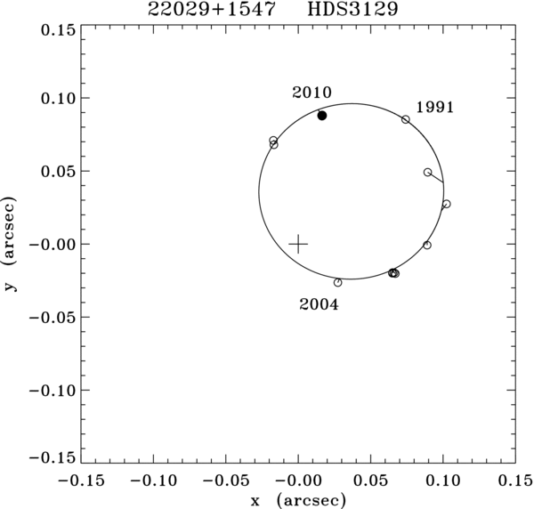
The second system for which we calculated a preliminary orbit is HDS 3129 (= WDS 22029 + 1547 = HIP 108842). In this case, the existing data in the 4th Interferometric Catalogue include one unsuccessful measure from the USNO speckle group (Mason et al. 1999), one successful measure by the same group (Mason et al. 2001a), a measure from the Russian team of Balega et al. (2007), the discovery observation of Hipparcos, and several of our own data points. The Balega et al. observation was taken at the SAO 6 m Telescope and yielded a very small separation measure for speckle—38 mas—a lucky occurrence as this point turns out to be an important measure in the orbit determination presented in Table 6. It is difficult to understand why Mason et al. (1999) did not detect the companion in their 1997 observation; this alone gives some uncertainty in the orbit that we present here. However, one of our own measures is from nearly the same time frame and was well above the diffraction limit at WIYN at that time. A graphical representation of this orbit is shown in Figure 8.
Figure 8. Orbit calculated here for HDS 3129 = HIP 108842 together with data from the literature and our measure from Table 1. The latter is shown with a filled circle. All points are drawn with line segments from the data point to the location of the ephemeris prediction on the orbital path. North is down and east is to the right.
Download figure:
Standard image High-resolution image
While Hipparcos reported the magnitude difference of this system to be 1.21 ± 0.65, both our own and the Balega speckle data indicate a substantially smaller value, less than 0.5 mag. Given the large uncertainty of the Hipparcos point and the relative consistency of the speckle measures, we find it more likely that the smaller value is correct. It is therefore quite possible that the quadrant has been incorrectly determined in some cases. Looking at the progression of the position angle starting with the discovery observation at 139°, there is a trend toward decreasing values through 1999. Then, for one measure in 2001 and three of the four measures in 2003, the quadrant appears reversed. All of these measures are ours and were stated as ambiguous when published. Therefore, we reversed these prior to computing our orbit. Our subsequent observations in 2007 were not ambiguous, nor is the measure in Table 1 here. We have not changed their position angles for the orbit calculation. Finally, the Balega point was reversed from 226° to 46° on the thinking that at small separation the assignment of the correct quadrant for a small magnitude difference is especially difficult.
The orbit yields a mass sum of 1.7 ± 0.8 M☉ when combined with the revised Hipparcos parallax, which is 10.78 ± 0.80 mas. The spectral type of the system is listed as F4V in SIMBAD, so that if the system indeed has a small magnitude difference, the pair should be in the neighborhood of F4V+F6V, implying a mass sum of approximately 2.8 solar masses. This is somewhat higher than the dynamical mass, but well within 2σ of that result.
5. CONCLUSIONS
We have presented nearly 500 speckle observations, 367 of which were resolved into two or more stars and 130 of which were not resolved. This group of observations is the first major data set using the new two-EMCCD arrangement with the DSSI at the WIYN Telescope. The astrometric measurement repeatability is estimated to be approximately 1.1 mas when the positional information from both channels is combined for a single measure, and the typical uncertainty in differential photometry is estimated to be 0.07–0.08 mag. Using the data presented here and existing data in the literature, first orbit determinations are made for two systems. In both cases, the dynamical mass sum, although fairly uncertain, is consistent or nearly consistent with what would be expected given the spectral type and magnitude difference of the system.
We thank the Kepler Science Office located at the NASA Ames Research Center for providing partial financial support for the upgraded DSSI instrument. It is also a pleasure to thank Dave Summers, Karen Bulter, Charles Corson, Jenny Power, Krissy Reetz, and Bill Binkert for their assistance at the telescope during our two runs at Kitt Peak, and the anonymous referee, for a thorough reading of the original manuscript. This work was funded by NSF grant AST-0908125. It made use of the Washington Double Star Catalog maintained at the U.S. Naval Observatory and the SIMBAD database, operated at CDS, Strasbourg, France.