


Abstract
We derive the longest uniform record of rotational intensities solar coronal magnetic field since 1968 and compare it with the heliospheric magnetic field (HMF) observed at the Earth. We scale the Mount Wilson Observatory and Wilcox Solar Observatory observations of the photospheric magnetic field to the level of the Synoptic Optical Long-term Investigations of the Sun/Vector Spectro Magnetograph and apply the potential field source surface model to calculate the coronal magnetic field. We find that the evolution of the coronal magnetic field during the last 50 yr agrees with the HMF observed at the Earth only if the effective coronal size, the distance of the coronal source surface of the HMF, is allowed to change in time. We calculate the optimum source surface distance for each rotation and find that it experienced an abrupt decrease in the late 1990s. The effective volume of the solar corona shrunk to less than one half during a short period of only a few years. We note that this abrupt shrinking coincides with other changes in solar magnetic fields that are likely related to the decrease of the overall solar activity, i.e., the demise of the Grand Modern Maximum.
Export citation and abstract BibTeX RIS
1. Introduction
Magnetic field of the visible solar surface, the photosphere, determines the structure of the solar corona, solar wind, and the heliospheric magnetic field (HMF; Cahill 1965) and, through them, controls the disturbances affecting the near-Earth space, for example, geomagnetic storms and aurorae. The photospheric magnetic field intensifies when new active regions like sunspots appear on the solar surface (Wang et al. 1989; Smith et al. 2003). The number of sunspots varies in cycles of 10–11 yr, but the height of these sunspot cycles also varies from cycle to cycle, indicating longer-term variability in solar activity. The height of sunspot cycles increased systematically during the first half of the twentieth century, leading to a maximum during cycle 19 in the late 1950s, now called the Grand Modern Maximum (GMM). Solar activity has declined since then, first rather slowly during cycles 20–22 but then, during the current cycle 24, the Sun's activity slowed to a lower level that was typical one hundred years ago, before the start of the GMM.
The magnetic field of sunspots (Hale et al. 1919) and the activity of the solar chromosphere (Ellerman 1919) were observed already since the rising phase of the GMM. However, the information on solar corona during those early decades is mainly based on proxy data like geomagnetic activity (Mursula et al. 2015, 2017) and momentary snapshot observations of the corona during solar eclipses (Tlatov 2010). Direct satellite observations of the solar wind started in the early 1960s, allowing for a greatly improved understanding of the structure of the HMFs. Understanding solar magnetic fields was further aided by continuous magnetograph observations of the photospheric magnetic field, which started soon after the start of the satellite era. Accordingly, almost the entire declining phase of GMM is covered by versatile magnetic observations, which now allow us to study the effects of this long-term decline of solar activity on the corona.
We know roughly how the structure of the coronal magnetic field is formed by the photospheric magnetic field (Petrie 2013; Wiegelmann et al. 2017; Mikić et al. 2018; Cheung et al. 2019), but the relation between the photosphere and the corona is complicated and time-variable. Moreover, because we still cannot directly measure the coronal magnetic field, most information on the coronal field is based on models using photospheric observations as their input. The most commonly used model of the coronal magnetic field is the potential field source surface (PFSS) model (Altschuler & Newkirk 1969; Schatten et al. 1969; Hoeksema et al. 1983), which assumes that there are no significant electric currents between the photosphere and the coronal source surface, and that the coronal magnetic field becomes radial at the source surface distance of about 1.5–3.5 solar radii (Rs). With these assumptions the coronal magnetic field between the photosphere and the source surface can be solved using the observed photospheric magnetic field as a boundary condition.
Several studies compare the coronal magnetic field derived from the PFSS model with heliospheric observations. Riley et al. (2006) concluded that magnetohydrodynamic (MHD) models require a lot of calculation power (and are required for modeling time-dependent structures), but yield rather little advance to the PFSS model, despite its simplicity. They noted that choosing the data set for the photospheric field may have a larger effect than choosing between the PFSS or the MHD model. Lee et al. (2011) compared coronal holes and open coronal flux derived from the PFSS model to coronal holes from extreme-ultraviolet (EUV) images and heliospheric observations of the open HMF flux. They derived the value of the source surface radius to be roughly the same, about 1.9 and 1.8 Rs, during the minima after solar cycles 22 and 23, respectively. Arden et al. (2014) concluded that a constant source surface of 2.5 Rs can reproduce the observed HMF flux during cycle 23. However, we have not been able to reproduce these results. Luhmann et al. (2013) used Global Oscillation Netwrok Group (GONG) data and both the PFSS model and the magnetohydrodynamics around a sphere (MAS) model to study the coronal geometry and solar wind sources during solar cycle 23, finding a fairly good agreement between the two models. Recently, (Koskela et al. 2017) showed that the PFSS model reliably produces the HMF sector structure. Moreover, adding horizontal currents (as in the current sheet source surface (CSSS) model; Koskela et al. 2019) or using an MHD model (Li & Feng 2018) does not improve the polarity match between the corona and the heliosphere. All these studies indicate that, despite its simplified assumptions (lack of currents and spherical source surface), the PFSS model can well produce the large-scale coronal magnetic field structure, even at different solar activity conditions.
The absolute value of the radial component of the HMF, also called the (unsigned) HMF flux density ϕHMF is a measure of magnetic energy emitted by the corona with the solar wind into the heliosphere. Because the total magnetic flux is conserved, the HMF flux through a sphere around the Sun is invariant of the sphere radius, and the initial HMF flux density at the site of HMF emission, the coronal source surface, decreases with radial distance inversely proportional to the area of a sphere (1/r2). Moreover, as HMF observations by the Ulysses probe over a large range of heliographic latitudes have shown that the HMF flux density is independent of latitude (Smith & Balogh 1995; Owens et al. 2008), the total HMF flux can be determined by a flux density measurement at any single point in the heliosphere.
A major challenge of studying the long-term evolution of the solar magnetic fields is imposed by the fact that the different magnetograph instruments yield quite different photospheric flux densities depending, e.g., on spectral and spatial resolution, data processing method, and the treatment of the unobserved solar poles (Riley et al. 2014). We have recently developed a new method for scaling the magnetograms from different instruments to each other in terms of harmonic expansion (Virtanen & Mursula 2017, 2019). This method can be used to scale any pair of photospheric field observations with a reasonable overlapping period.
In this Letter we study the long-term evolution of the coronal field using the PFSS model and Wilcox Solar Observatory (WSO) and the Mount Wilson Observatory (MWO) separately to the more recent high-resolution observations by the Synoptic Optical Long-term Investigations of the Sun/Vector Spectro Magnetograph (SOLIS/VSM). We compare the total flux of the coronal field to the HMF measured at Earth's orbit. The Letter is structured as follows. In Section 2 we present the data sets and methods we use. In Section 3 we discuss the long-term evolution of the coronal field, and in Section 4 we summarize our results.
2. Data and Methods
We use hourly HMF and SW data observed around the Earth's orbit by several satellites since the 1960s. These data are scaled to 1 au, and collected to the NASA/NSSDC OMNI-2 database (King & Papitashvili 2005). These data provide the longest single-point measurement in the heliosphere with variable, but mostly sufficient data coverage. In order to study long-term variations, we use here HMF flux density averages over one solar rotation (Carrington period of 27.2753 days). When calculating the rotational averages in this article we require a 20% data coverage of hourly values (minimum of 131 values out of 654) for each rotation. If the coverage is smaller than this, the corresponding rotation is neglected.
We use WSO synoptic maps of the photospheric magnetic field since 1976. WSO magnetograph is a low-resolution device (3' aperture size), and suffers from saturation (Svalgaard et al. 1978). This affects the intensity of the measured field, but the erroneous absolute level has largely been corrected by the new scaling method (Virtanen & Mursula 2017). The same instrumentation has been operating at WSO since the start of observations, which makes the WSO database homogeneous and, therefore, very useful for long-term studies. We neglect rotations 1905–1944 (1996 January–1998 December) and 1973–1978 (2001 February–2001 June) when WSO data is known to be erroneous (Virtanen & Mursula 2016).
As a second data set of the photospheric magnetic field we use the calibrated synoptic maps since 1967 from the MWO. Note that the data of the period of 1967–1974 became publicly available only in 2018, and have not been used for long-term studies so far. There were instrumental updates at MWO in 1974, 1982, 1994, and 1996, and MWO observations were terminated in 2013 January. We use only full synoptic maps (with no data gaps) in their original published format without any modifications. (For more detailed description of magnetograph data, see Virtanen & Mursula 2016, 2017 and references therein.)
We scale the WSO and MWO data sets to the absolute level of the SOLIS/VSM instrument, which measured the photospheric magnetic field in 2003–2017. In the harmonic scaling method (Virtanen & Mursula 2017), a linear regression is derived between the corresponding harmonic coefficients of  and
and  (see Section 2.2) for any two data sets using rotations included in the overlapping time interval. For each pair of data sets, we calculate the scaling matrices, for example, Gmn(MWO → SOLIS) and Hmn(MWO → SOLIS), which are used to multiply the harmonic coefficients of the data set to be scaled (MWO) to the level of the other data set (SOLIS). We note that the Gmn and Hmn are constant in time. We hereafter denote the WSO (MWO) data scaled to SOLIS/VSM as WSOVSM (MWOVSM)
2.1. Heliospheric Flux Density
Ulysses probe observations (Smith & Balogh 1995) have shown that  is independent of latitude. Using this, together with the radial decay of Br ∼ r−2, we end up with the following form for the total unsigned flux:

where the average is taken over one solar (Carrington) rotation of 27.2753 days.
There are different methods to derive the magnetic flux density in the heliosphere. The challenge is that the distribution of Br includes both positive and negative values. A simple average of  overestimates the unsigned flux in case of high-resolution data, mainly because of noise, and underestimates it in case of very low-resolution data, where opposite HMF sectors (polarities) are effectively averaged (Smith 2011).
Erdös & Balogh (2012) suggested that all deviations from the Parker spiral field are fluctuations that should be removed before calculating the rotational averages of the radial field. In order to remove these fluctuations, the rotational averages of  are calculated from the component aligned along the Parker spiral field.
Parker's model for the HMF is

where Bss is the source surface flux density, rss is the source surface radius, vr and vϕ are the radial and azimuthal velocity components of velocity, r is the heliocentric distance, λ is the heliographic latitude, and Ω the solar angular velocity. The HMF component along Parker's spiral is then

and the rotational averages of the unsigned HMF flux  are obtained as follows:

(Note that six-hour averages of  and
and  are used in Equation (3) in order to reduce fluctuations, as suggested by Erdös & Balogh 2012).
Lockwood et al. (2009) developed a sophisticated method of removing kinematic effects, which relates to variable solar wind velocity and the tangential magnetic field component. However, they concluded that a more simple method of first deriving 24 hr averages of signed Br and then averaging over the solar rotation time gives close to the same result as the sophisticated method. We use here this simple method in order to calculate another version of the HMF flux density at 1 au as follows:

Figure 1 shows ϕau according to the methods by Lockwood et al. (2009) and by Erdös & Balogh (2012). The Lockwood method yields a systematically larger  but the difference between the two methods is very small (about 0.12 nT).
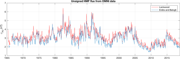
Figure 1. Unsigned open flux at 1 au using the method by Lockwood et al. (2009) and the method by Erdös & Balogh (2012).
Download figure:
Standard image High-resolution image2.2. PFSS Model
The PFSS model assumes that, at a certain distance called the source surface (rss), the radially out-flowing plasma takes over the magnetic field and the field becomes radial. Thereby, the outer boundary condition of the PFSS model requires that the field is radial at rss. The PFSS solution for the radial component of the coronal magnetic field between the photosphere and the source surface is
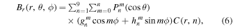
where the radial functions C(r, n) are
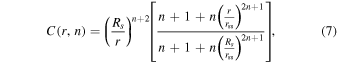
and  are the associated Legendre functions, gnm and hmn are the harmonic coefficients of the spherical harmonic expansion, Rs is the solar radius, r is the radial distance, and θ is the co-latitude (polar angle). (The nonphysical magnetic monopole term n = 0 is neglected.) For a more detailed description of the PFSS model and the method of deriving harmonic coefficients gmn and hmn, see Virtanen & Mursula (2016).
3. Long-term Evolution of the Source Surface Radius
Here we use the long-term photospheric data series WSOVSM and MWOVSM as input to the PFSS model in order to study the long-term evolution of the coronal magnetic field. The larger the source surface radius of the PFSS model is, the more of the coronal field lines close within the corona and the smaller the HMF flux density will remain. This is seen in Figures 2(a) and (b) where we have plotted the mean coronal magnetic flux density ( ) scaled from the coronal source surface to 1 au for three coronal source surface distances (
 ) for WSO since 1976 and for MWO in 1967–2013. (Source surface fluxes were scaled to the distance of 1 au using the
  radial decrease of the flux density). The overall mean values of the flux densities ϕss for the three rss values of 3.7, 1.9, and 1.3 nT for WSOVSM, and 3.8, 2.0, and 1.4 nT for MWOVSM. (The small difference is due to the somewhat different time intervals). Figures 2(a) and (b) also include the
  reproduced from Figure 1. The mean of
  over the whole time interval is 2.7 nT, showing that the overall best-fitting value of rss is between 1.5 and 2.5 Rs.
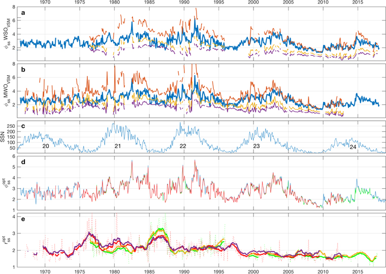
Figure 2. Panel (a): HMF flux observed at 1 au ( thick blue line) together with coronal flux densities
  (scaled to 1 au) for WSOVSM data and for rss values of
  (red),
  (yellow), and
  (purple). Panel (b): the same as Panel (a), but for MWOVSM data. Panel (c): monthly sunspot numbers. Panel (d): HMF flux density
  (blue) and the corresponding optimum coronal flux densities
  for WSOVSM (green) and MWOVSM (red) data. Panel (e): optimum source surface radius rEBss for WSOVSM (green) and MWOVSM (red; dotted lines depict rotational values and thick lines the 13-rotation running means) and (the 13-rotation running means of) the optimum source surface radius rLss for WSOVSM (yellow) and MWOVSM (purple).
Download figure:
Standard image High-resolution imageFigures 1, 2(a) and (b) show that the maxima of ϕau occur in the early declining phase of solar cycles 21–24 (in 1982, 1991, 2003, and 2014/2015) and the minima of ϕau around sunspot minima. (ϕau shows only a weak peak in 1974 during solar cycle 20). The timings of the ϕss maxima agree fairly well with ϕau maxima for all rss values, but the timings of ϕss minima are quite different for different rss values (Virtanen & Mursula 2019). For rss = 1.5 Rs MWOVSM shows minima around sunspot minima in 1986, 1996, and 2009 and WSOVSM in 1987 and 2009, in a good agreement with ϕau. However, for rss = 2.5 Rs and rss = 3.5 Rs neither MWOVSM nor WSOVSM show minima at the same time as ϕau, i.e., at sunspot minima, but only much later, in the ascending phase or even at the maximum of the next cycle.
The maximum-time (minimum-time) level of ϕau has systematically decreased from cycle 22 maximum to cycle 24 maximum (from mid-1980s to mid-2000s, respectively). This long-term decrease of the observed HMF flux density in recent decades is well documented (Smith & Balogh 2008; Lockwood 2013). The same systematic decline is seen in ϕss in Figures 2(a) and (b) for all values of rss from cycle 22 until recently. However, the relative reduction is clearly larger in ϕss than in ϕau during the same time interval. For rss = 1.5 Rs the corresponding flux density ϕ1.5 agrees very well with ϕau during the last 20 yr but greatly exceeds that in the earlier decades. The closest match in the 1980s is found between ϕ2.5 and ϕau but ϕ2.5 remains significantly below ϕau during the last 20 yr. These systematic differences between ϕss and ϕau reflect the fact that the long-term evolution of the modeled coronal field ϕss does not fit with the observed flux density ϕau using any constant value of the source surface radius. The same conclusion was made by Wang et al. (2000) ,who used a constant rss for the early decades, but noted that cycle 23 cannot be reproduced with the same value.
In order to solve this problem we now calculate ϕss so that rss does not have to be constant but can vary in time. For each rotation, starting from rss = 1.05 Rs (for which ϕss exceeds ϕau for all rotations) we increase rss in steps of 0.05 Rs, thus reducing ϕss until it agrees with ϕau for that rotation. Using this method we can find an optimum source surface distance  and an optimum flux density
  , which closely agrees with
  for that Carrington rotation. Figure 2(d) shows the perfect match between
  and the corresponding
  for each rotation. Figure 2(e) shows the rotational values of rssopt for
  , which vary from
  in 2017 to
  in 1987 for WSOVSM and from
  in 2009 to
  in 1980 for MWOVSM. Figure 2(e) also includes the 13-rotation running means of rssopt for both
  and
and  , which both depict maxima around the three sunspot minima in 1976–1977, 1986–1987, 1996–1997 (and a smaller hump in 2006 and 2009 in
  ), but no other systematic changes during the sunspot cycle.
The first two of these maxima are about 30%–50% above the mean level of rssopt in the 1980s and 1990s.
The rssopt values in Figure 2(e) depict an interesting long-term evolution. At the start of the time interval studied, in the late 1960s and early 1970s, the rssopt values were slightly lower, about  , than in the 1980s and 1990s. However, this is only based on MWOVSM data and is therefore less certain than those later results which both MWOVSM and WSOVSM can verify. These two series agree on the considerably lower level of rssopt values during the last 20 yr than in the three earlier decades. In fact, there is a step-like decrease in rssopt after the sunspot minimum in 1996–1997, and a weakly decreasing trend thereafter. (Unfortunately, the WSO data is erroneous in the late 1990s over this time interval and is left out from Figure 2(e); see Section 2). Note that this decreasing trend in rssopt during the last 20 yr is fairly linear, with only weak solar cycle related variations. Even the all-time minimum of
  in 2009 (see Figure 2(d)) is very well reproduced by
  with only a small increase in the corresponding rssopt.
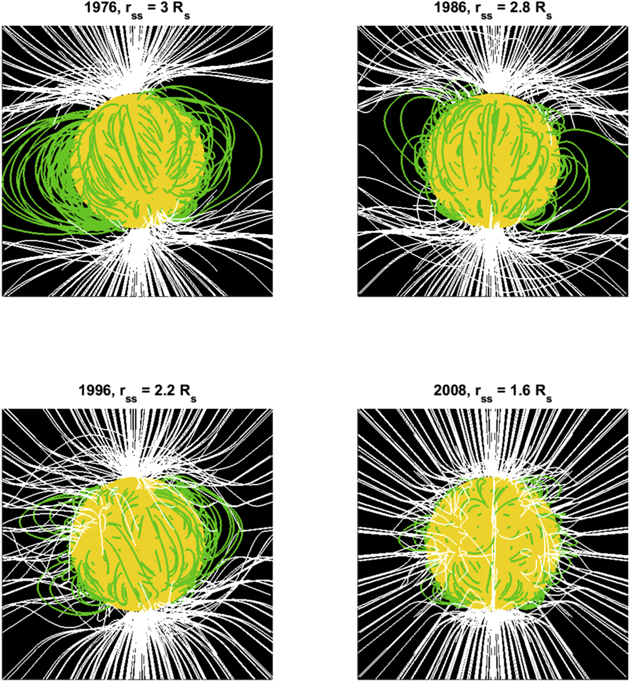
Figure 3 shows one sample of a coronal field configuration during each of the four sunspot minima (in 1976, 1986, 1996, and 2008) using MWOVSM data and the corresponding rssopt values. Figure 3 shows that the structure of the coronal magnetic field has notably changed from the minimum in 1976 to the minimum in 2008. The coronal structure in 1976 depicts a large volume of closed magnetic field lines (magnetic loops), with a large fraction of those field lines connecting high northern latitudes with high southern latitudes. These long field lines extend quite far from the solar surface at the equator, indicating a large source surface distance. On the other hand, during the minimum in 2008 there are hardly any of such long field lines connecting the two hemispheres at high latitudes, and the closed field lines extend much lower in the corona than during the earlier minima.
Figure 3. Coronal magnetic field line configuration using MWOVSM data and annual average of the optimum source surface distance rssopt during solar minima in 1976 (CR1643,  ), 1986 (CR1781,
  ), 1996 (CR1917,
  ), and 2008 (CR2077,
  ).
).
Download figure:
Standard image High-resolution image
4. Summary
In this Letter we have shown that the coronal source surface distance has notably decreased from the mid-1970s until recently. This has also modified the topology of the coronal magnetic field so that the field lines now become radial at a lower altitude (smaller distance) than they did 20–50 yr ago. This shrinking of the coronal source surface from about 2.0 to  from the late 1970s until mid-1990s to about
  in the last decade implies that the volume of the solar corona, where the magnetic field is the dominant form of energy, has reduced to less than one half during the last 20 yr. We find that a large fraction of this shrinking occurred as a step-like decrease in the late 1990s, in the early ascending phase of cycle 23. Similar abrupt changes roughly at the same time have been noted, e.g., in the distribution of sunspots (Lefèvre & Clette 2011; Clette & Lefèvre 2012), in sunspot magnetic field strength (Tapping & Valdés 2011; Watson et al. 2011), and in the relation between sunspot number and several solar EUV proxies (Lukianova & Mursula 2011; Livingston et al. 2012). Moreover, as seen in Figures 2(a), (b) and (d), the strength of the HMF, the open solar magnetic field, has significantly decreased over the same time interval (Wang et al. 2009; Hathaway & Rightmire 2010; Virtanen & Mursula 2019). These changes in the solar magnetic fields are most likely related to the decrease of the overall solar activity that mark the end of the exceptional period of the GMM of the twentieth century.
We acknowledge the financial support by the Academy of Finland to the ReSoLVE Centre of Excellence (project No. 307411). Wilcox Solar Observatory data used in this study were obtained via the website http://wso.stanford.edu courtesy of J.T. Hoeksema. This study includes data from the synoptic program at the 150 Foot Solar Tower of the Mt. Wilson Observatory, which is acknowledged. Data were acquired by SOLIS instruments operated by NISP/NSO/AURA/NSF.
Data used in this study was obtained from the following web sites:
WSO: http://wso.stanford.edu.
MWO: ftp://howard.astro.ucla.edu/pub/obs/synoptic_charts/fits/.
SOLIS/VSM: http://solis.nso.edu/0/vsm/vsm_maps.php.