


ABSTRACT
A condensate cloud on Titan identified by its 220 cm−1 far-infrared signature continues to undergo seasonal changes at both the north and south poles. In the north, the cloud, which extends from 55 N to the pole, has been gradually decreasing in emission intensity since the beginning of the Cassini mission with a half-life of 3.8 years. The cloud in the south did not appear until 2012 but its intensity has increased rapidly, doubling every year. The shape of the cloud at the south pole is very different from that in the north. Mapping in 2013 December showed that the condensate emission was confined to a ring with a maximum at 80 S. The ring was centered 4° from Titan's pole. The pattern of emission from stratospheric trace gases like nitriles and complex hydrocarbons (mapped in 2014 January) was also offset by 4°, but had a central peak at the pole and a secondary maximum in a ring at about 70 S with a minimum at 80 S. The shape of the gas emission distribution can be explained by abundances that are high at the atmospheric pole and diminish toward the equator, combined with correspondingly increasing temperatures. We discuss possible causes for the condensate ring. The present rapid build up of the condensate cloud at the south pole is likely to transition to a gradual decline from 2015 to 2016.
Export citation and abstract BibTeX RIS
1. INTRODUCTION
A primary goal of the Cassini mission is to follow the seasonal evolution of Titan's atmosphere over half a Saturnian year. By the planned end of the mission in 2017, Cassini will have covered almost two seasons on Titan in 13 years, spanning winter and spring in the north and summer and autumn in the south. Already after 10 years at Saturn, large seasonal trends are evident on Titan including latitude variation of temperatures, hazes, clouds, and gases (Teanby et al. 2008, 2010, 2012; Coustenis et al. 2010, 2015; Achterberg et al. 2011; West et al. 2011; Bampasidis et al. 2012; Cottini et al. 2012a; Jennings et al. 2012a; Vinatier et al. 2012, 2015). Seasonal phenomena are most pronounced at the poles where the variation in warming and cooling is greatest. While changes in Titan's north have been gradual, in the south they have been rapid and dramatic. In 2012, after the south pole entered into shadow during winter, both visible and infrared cloud signatures suddenly developed (Jennings et al. 2012b; West et al. 2015). Between mid-2011 and late 2014, the polar temperature at the 1 mbar level (180 km) had decreased from 160 to 120 K (Teanby et al. 2012; Achterberg et al. 2014; de Kok et al. 2014; Coustenis et al. 2015; Vinatier et al. 2015).
Changes have been fast in a polar condensate cloud seen at 220 cm−1 in far-infrared spectra from Cassini's Composite Infrared Spectrometer (CIRS; Flasar et al. 2004). This cloud is most predominant in the winter polar regions and is not seen at mid-latitudes or the equator. Although its composition remains a mystery, the condensate is thought to come from gases originally formed at high altitude that are transported by global circulation to the winter pole where they collect and are protected from dissociation in the winter shadow (see, for example, Teanby et al. 2012). The gases move downward, eventually condensing in the stratosphere. Originally discovered by Voyager (Kunde et al. 1981; Coustenis et al. 1999), the 220 cm−1 feature has been the subject of many studies using CIRS data (Flasar et al. 2004; de Kok et al. 2007, 2008; Samuelson et al. 2007; Anderson et al. 2012; Jennings et al. 2012a, 2012b). We previously reported the decline in radiance of the cloud in Titan's north (Jennings et al. 2012a) and then its sudden appearance, in 2012, at the south pole (Jennings et al. 2012b). The condensate cloud is only known from its spectral signature in the far-infrared; its counterpart in visible and near-infrared images has not yet been identified.
2. OBSERVATIONS
Our data for this study were taken from 76 flybys from 2004 December to 2015 March. Most of the flybys included both the north and south polar regions. We included data from three types of observations. First, using spectra from the whole mission, we measured changes in the average intensity at 220 cm−1 near both poles. Second, on 2013 December 1, we mapped the 220 cm−1 cloud emission in the south. Third, on 2014 January 2, we mapped gas emissions in the south. CIRS is a Fourier transform spectrometer with three focal planes (Flasar et al. 2004). Focal plane FP1 covers 10–600 cm−1, FP3 covers 600–1100 cm−1, and FP4 covers 1100–1500 cm−1. We used spectra from FP1 to study the 220 cm−1 feature, FP3 to study gas emissions, and FP4 to derive temperatures. CIRS' spectral resolution can be selected from 0.5 to 15 cm−1. Because the 220 cm−1 feature is 30 cm−1 wide, we used 15 cm−1 for the FP1 observations. For FP3 and FP4, we needed at least 3 cm−1 resolution to separate spectral lines. The fields of view in FP1 and FP3 are 2.5 and 0.3 milliradians, respectively. The spacecraft range was almost always less than 200,000 km for the FP1 north and south measurements, 70,000 km for the 2013 December 1 mapping, and 300,000 km for the 2014 January 2 mapping. For the long -range FP1 observations, the field of view was allowed to encompass both disk and limb. For both FP1 and FP3 mappings, the field of view was kept entirely on the disk. During mapping the emission angle was generally below 50°. For the 2013 December 1 data set the spectra were from a flyby in which the FP1 field of view followed a linear path from 40 S latitude, 180 W longitude to 40 S latitude, 20 W longitude, and came within 0 5 of the pole. For the 2014 January 2 data set, the FP3 observations were arranged in a two-dimensional grid covering southern latitudes from the pole to 40 S.
3. DATA ANALYSIS
We constructed three data sets, one from the north and south polar intensity observations, and one each from the FP1 and FP3 mapping observations. For the FP1 polar intensity data set, we averaged, for each flyby, spectra between 70° and 90° latitude either in the north or south. The radiances of the condensate cloud were determined by subtracting the continuum from the 220 cm−1 peak emission. Because of the varying field of view, emission angle, and tangent height, the cloud radiances were corrected for observing geometry following the procedure described by Jennings et al. (2012b). In each spectrum, the radiance of the 220 cm−1 cloud was ratioed to the radiance in the C3H4 band at 325 cm−1. For the December 1 and January 2 maps, the 220 cm−1 peak-minus-continuum radiances were used without ratioing to 325 cm−1. For both maps the spectra were averaged in 25 bins. The center longitudes in the January bins were selected to follow the path of the December map to facilitate comparison. We retrieved gas abundances from the January spectra after first deriving the temperature profile from an inversion of the 1306 cm−1 CH4 band in FP4, following a procedure described elsewhere (Achterberg et al. 2011; Cottini et al. 2012b; Coustenis et al. 2015).
4. RESULTS AND DISCUSSION
Evolution over mission. Figure 1 shows our measured emissions at 220 cm−1 as a function of season. In the figure, the northern data are used to represent winter and spring, while the southern data represent summer and autumn. The northern emission has continued its gradual decay. The trend is matched well by an exponential decrease with a half-life of 3.8 Earth years, or 1.5 Titan months. In the south, the behavior of the 220 cm−1 cloud has been completely different. The strength of the emission in the vicinity of the south pole has increased dramatically since 2012 and now exceeds the brightest ever seen in the north. The south pole emission approximately doubles every year, or 0.4 Titan months. It is clear that if the evolution of the cloud in the south is to mirror that in the north, then the steep increase in the south cannot go on indefinitely. Extrapolating the exponential behavior in the north backwards toward mid-autumn implies that the transition in the south from rapid increase to gradual decrease can be expected to occur in 2015–16. Most likely, the process that is filling the stratosphere with condensate cloud during the initial rise will taper off and the cloud will slowly evaporate (as temperatures rise) and rain out during the southern winter.
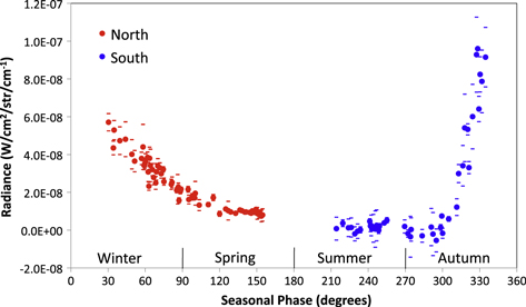
Figure 1. North and south polar radiances at 220 cm−1 shown with respect to Titan season. In this plot, winter and spring are represented by Titan's north while summer and autumn are represented by Titan's south. Zero seasonal phase is at winter solstice. A 30° increment corresponds to one Titan month. Data were recorded during 2004–2015. Error bars are indicated with dashes. The radiances are scaled to 2005 March 31, when the highest radiance was recorded in the north.
Download figure:
Standard image High-resolution imageMorphology in the south. In addition to its rapid emission rise at the south pole, the 220 cm−1 feature exhibits a complex spatial structure. Its shape and extent are distinctly different from the broad hood always seen in the north. By mid 2013, we began to suspect that the condensate cloud was confined poleward of 70 S and was not uniform. During the flyby on 2013 December 1, CIRS was able to map the emission in detail. The field of view was scanned across the south pole on a path almost directly away from the Sun. The result is shown in Figure 2. The 220 cm−1 emission has two latitudinal peaks with a deep minimum at the pole. The two peaks signify a ring morphology that brackets the visible vortex cloud seen by the Cassini Imaging Science Subsystem and Visible and Infrared Mapping Spectrometer (VIMS) in 2012 (de Kok et al. 2014; West et al. 2015). The center between the peaks is shifted 4° from the geographic pole, corresponding to the atmospheric tilt identified earlier by Achterberg et al. (2008) from the temperature field in the north. The radius from the atmospheric axis of the 220 cm−1 emission ring is about 10° of latitude. The atmospheric tilt is toward the Sun. Achterberg et al. (2008) conjectured that the atmospheric axis seeks alignment to the Sun to maximize pumping of the meridional circulation. Such pumping may be especially strong during the twice-annual build up of circulation at the autumnal pole. We see, in fact, that the tilt was almost directly toward the Sun at the time of the strong polar vortex in early 2014, one Titan month before solstice.
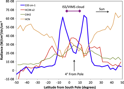
Figure 2. 220 cm−1 cloud emission observed along a track across the south pole on 2013 December 1 compared with emission from HC3N, C4H2, and HCN gases. Latitudes are referred to the geographic pole. The position of the atmospheric pole is indicated, tilted 4° from the geographic south pole (Achterberg et al. 2008). Latitudes are at the surface, i.e., not corrected for the altitude of line formation. The HC3N radiances are shown as twice the measured values for ease of comparison.
Download figure:
Standard image High-resolution imageHaving detected the anomalous structure of the 220 cm−1 emission near the south pole, we looked for similar configurations in gas emissions. Figure 2 shows the profiles of HC3N, C4H2, and HCN on 2014 January 2. This flyby was the closest one in time to 2013 December 1 that included an FP3 map in the south. We found that the emissions from HC3N and C4H2 did indeed have ring-shapes, but that they were more bull's-eye shaped with a peak in the center and a ring at a radius of about 20° from the pole. Two-dimensional maps of HC3N and C4H2 emission, shown in Figure 3, show the distinctive ring and central peak. As can be seen in both Figures 2 and 3, the gas emissions are shifted toward the Sun by the 4° atmospheric tilt. A comparison in Figure 2 of the gas profiles with the 220 cm−1 condensate profile reveals the curious fact that the ring of peak condensate emission coincides with the minimum at 10° radius in the gas profiles. As can be seen in that figure, the HCN emission also dips at this radius. However, HCN has a different overall shape from the other two gases; it instead follows the temperature rise toward lower latitudes. We note that other secondary gases such as C3H4 and C6H6 also show the bull's-eye structure, whereas the primary gases C2H2, C2H6, and CO2 follow the temperature rise (see Coustenis et al. 2015). HCN appears to be intermediate to these two categories.

Figure 3. Maps of emission from gaseous C4H2 (a) and HC3N (b) in the vicinity of Titan's south pole. Dashed latitude circles are separated by 15°. Longitudes are oriented with 180° toward the right in the direction of the Sun. Red is brighter, and blue is dimmer. The asymmetric brightness in the rings is mostly due to emission angle variation.
Download figure:
Standard image High-resolution imageClearly, there were significant changes taking place at the south pole at the beginning of 2014. Figure 4 offers some hints at what might have been going on. In the figure, the 220 cm−1 emission is plotted together with the HC3N and C4H2 abundances. Temperatures at 1 mbar are also shown. The 220 cm−1 ring is at 80 S and this is also where the temperature begins to rise above its polar minimum. The C4H2 and HC3N abundances both have a peak at the pole and a steep fall-off toward lower latitudes, reaching about 0.2 of their peak values at 80 S and disappearing by about 60 S. One explanation for the bull's-eye shape of the gas emission profiles in Figure 2 is that the abundance is highest at the pole where the emission is greatest and falls off quickly with latitude. At 80 S, the decreasing abundance causes low emission. Beyond that, the steep temperature increase overcomes the decreasing abundance and creates the ring at 70 S. This scenario works for the gases, but it does not explain why the 220 cm−1 emission has such a different shape, with a maximum at 80 S and a minimum at both 90 S and at 70 S. One possibility is that the distribution of the condensate is different from that of the gases, in altitude as well as latitude. The condensate will be below the altitude where saturation occurs, and therefore its condensate opacity can be expected to peak at levels below where the gas opacities are greatest. Nitriles and hydrocarbons tend to condense at or below 300 km. de Kok et al. (2014) identified HCN ice in the vortex cloud seen at the south pole at 300 km in 2012. (In the north, the condensate has been below 150 km (de Kok et al. 2007).) On the other hand, in 2012 the southern polar gases were concentrated above 300 km (Vinatier et al. 2015). The gas and condensate emissions might therefore be probing two separate heights with different latitude dependences of density and temperature. For example, the deep polar temperature well is accompanied by strong circumpolar winds (Achterberg et al. 2014) and these may form a barrier to mixing across 80 S. The barrier may be indicated in the C4H2 and HC3N abundances, which appear to have a shoulder or dip at around 80 S. Condensates at lower altitudes may be impeded against migrating across the barrier. It is also possible that the coincidence at 80 S of the maximum of the 220 cm−1 emission with the minimum in the gas emissions (Figure 2) indicates where condensation is taking place. Also, if the condensate particle size increases at the pole where the gases are more abundant, the central minimum there may be caused by faster rain-out and smaller extinction cross-sections per unit of condensate mass.

Figure 4. 220 cm−1 emission on 2013 December 1 compared with abundances of HC3N and C4H2 on 2014 January 2. The temperature profile is for 1 mbar (180 km altitude) on 2014 January 2. All curves are normalized. The peak 220 cm−1 radiance is 6.0 × 10⁻⁸ W/cm2/str/cm−1. The peak gas volume mixing ratios are 1.65 × 10⁻⁷ for HC3N and 7.9 × 10⁻⁸ for C4H2. The atmospheric axis is at −90 latitude (the 4° tilt has been removed) and latitudes are at 1 mbar altitude. Dashed lines are 1σ errors. Because of the increased errors near the pole, the small variations in the abundances at the pole are not significant.
Download figure:
Standard image High-resolution image
Cloud composition. We previously speculated that the condensate is of nitrile origin (Coustenis et al. 1999; de Kok et al. 2008) based on its confinement to polar regions and the correlation of its seasonal behavior with HC3N (Jennings et al. 2012a, 2012b). Recently, de Kok et al. (2014) demonstrated, using VIMS spectra, that the visible vortex cloud at the south pole is composed, at least in part, of HCN ice. Based on its condensation properties and availability, de Kok et al. (2008) posited that HCN is a major source for the 220 cm−1 material. HCN polymers may form in the 300 km cloud and migrate downward and thereby contribute nitriles to the condensate. Polymerization of HCN has been studied extensively (Bonnet et al. 2013, 2015), but we do not know that it will result in a spectral line at 220 cm−1. The condensate is probably a mixture of complex substances. The 220 cm−1 emission band may arise from the motion of a particular group of atoms that is attached to a variety of large molecules, i.e., it may not be due to a single molecular species.
We acknowledge support from NASA's Cassini mission and Cassini Data Analysis Program.