


ABSTRACT
We have carried out a comparative study of the predicted solar wind based on the flux tube expansion factor computed using the current sheet source surface (CSSS) model and the potential field source surface (PFSS) model, with the aim of determining whether the CSSS model represents the solar wind sources better than the PFSS model. For this, we obtained the root mean square errors (RMSEs) and the correlation coefficients between the observed solar wind speed and that predicted by the models, the ratio of RMSEs between the two models, and a skill score. On average, the CSSS predictions are more accurate than the PFSS predictions by a factor of 1.6, taking RMSE as the metric of accuracy. The RMSEs increased as the solar cycle progressed toward maximum, indicating the difficulty in modeling the corona as the global field becomes more complex. We also compared the WSA/ENLIL predictions for a few Carrington rotations; the Wang–Sheeley–Arge (WSA) model makes use of the PFSS extrapolations to model the wind source. We found that the average value of RMSE ratio between the CSSS and the WSA/ENLIL predictions was about 1.9, implying that the CSSS predictions are nearly twice better than the WSA/ENLIL predictions, despite the simplicity of the CSSS model compared to ENLIL. We conclude, based on the present analysis, that the CSSS model is a valid proxy for solar wind measurements and that it improves upon existing commonly used methods of wind prediction or proxy analysis.
Export citation and abstract BibTeX RIS
1. INTRODUCTION
Solar wind, a phrase coined by Parker (1958) who developed a theoretical explanation of the solar corpuscular emission postulated by Biermann (1951), was detected by MARINER observations more than half a century ago (Neugebauer & Snyden 1966). Theoretical studies and numerical modeling, along with numerous spacecraft missions since then, have established the dual nature of solar wind as having a fast component (speed > 500 km s−1) and a slow component (speed < 450 km s−1), although recent works (Elliot et al. 2012; Cranmer et al. 2013) suggest wind composition as a better discriminant for the two types of wind. Studies of the elemental and ionic compositions of slow wind have led to the suggestion of a different nomenclature for the two types of solar wind: steady and unsteady (Zurbuchen et al. 1999, 2002). It was also established that "fast" wind originates from coronal holes—regions of open magnetic field configuration (Zirker 1977). However, the origin of the "slow" component is not very well understood and is a much debated topic in solar physics (Fisk et al. 1998; Zurbuchen et al. 1999; Neugebauer et al. 2002; Ohmi 2003; Cranmer et al. 2013). The general understanding is that "slow" wind originates from regions of closed—both unipolar (pseudostreamers: Hundhausen 1972; Zhao & Webb 2003; Crooker et al. 2012) and bipolar—magnetic field configuration as suggested by their physical properties, which are markedly different from those of fast wind.
It has been suggested (Wang & Sheeley 1990) that all solar winds arise from coronal holes—the fast wind from the center and the slow wind from the boundaries—from correlation studies of solar wind speed (SWS) with the rate of flux tube expansion (FTE) within a region between photosphere and corona. Using this concept Arge & Pizzo (2000) obtained an empirical relationship between SWS and FTE, and used it for solar wind prediction (Wang–Sheeley–Arge (WSA) model: Arge & Pizzo 2000). The WSA model, built on the potential field source surface (PFSS) model, provides the ambient solar wind conditions at the inner boundary of the space weather prediction model ENLIL (Pizzo et al. 2011; Schultz 2011). WSA/ENLIL provides one- to four-day advance warnings of geomagnetic storms from quasi-recurrent solar wind structures and Earth-directed coronal mass ejections (CMEs), with an error of one to two days. The major single source contributing to this error is the uncertainty in the "background" solar wind provided by the WSA model, which is caused mainly by intrinsic flaws of the PFSS model. SWPC's current efforts are aimed at reducing the error in CME arrival time prediction to 6–8 hr and improving the inner boundary conditions for ENLIL (Pizzo et al. 2011; Schultz 2011).
The purpose of this Letter is to assess the accuracy of solar wind predictions of the current sheet source surface (CSSS) model (Zhao & Hoeksema 1995) by comparing it with near-Earth measurements and determine whether the CSSS model represents solar wind sources better than the PFSS model. We describe the two models in Section 2 and the data and methodology in Section 3. The results are summarized in Section 4, followed by a discussion and our conclusion in Section 5.
2. CSSS AND PFSS MODELS
Since direct observation of the coronal magnetic field is challenging and extremely limited, one has to resort to models that extrapolate the observed photospheric magnetic fields to the corona to study solar wind source regions. The most popular model is the PFSS model developed, independently, by Schatten et al. (1969) and Altschuler & Newkirk (1969). In this model, the corona is assumed to be current-free between the photosphere and the source surface (an arbitrary spherical surface called the Alfvén critical point; Parker 1958) beyond which plasma begins to control the magnetic field. The source surface is conventionally placed at a heliocentric distance of 2.5 R☉ (Hoeksema 1984), though Lee et al. (2011) found that distances as low as 1.5 R☉ yielded better comparison with observations during solar minima. All the magnetic field lines are constrained to be open and radial at the source surface and the coronal magnetic field is computed from a scalar potential obeying Laplace's law and according to the Parker spiral (Parker 1958). In addition to building the WSA model (Arge & Pizzo 2000), the PFSS model has been used extensively to address a variety of problems (e.g., Hoeksema 1984; Schrijver & DeRosa 2003; Luhmann et al. 2009).
The corona is not strictly current-free. Particularly, above 1.5 R☉ the existence of large-scale plasma structures (e.g., loop-like condensations) suggest appreciable interactions between the magnetic field and plasma (Zhao & Hoeksema 1993; Suess et al. 1998; Suess 2000). Therefore, the potential field approach in the PFSS model is an oversimplification of the real corona. Poduval & Zhao (2004) have shown that limitations of the PFSS model introduce significant uncertainties into the footpoint locations of source regions of the order of a few tens of degrees in longitude.
Assuming electric currents to be flowing perpendicular to gravity everywhere in the corona, Bogdan & Low (1986) have shown that a solution to the magnetostatic equilibrium can be obtained by solving a partial differential equation in an atmosphere with 1/r2 gravity in spherical geometry. The general solutions to this equation can be expanded as spherical harmonics similar to the PFSS model. The structures produced by the presence of electric currents will be computed in a self-consistent manner by the force-balance equation (Bogdan & Low 1986; Neukirch 1995). Based on this concept, Zhao & Hoeksema (1995) developed a CSSS model that includes effects of horizontal and sheet currents and a source surface.
Figure 1 depicts the geometry of the CSSS model (Zhao & Hoeksema 1995). Two spherical surfaces, the cusp surface and the source surface, divide the corona into three regions. Located at around 2.5 R☉, the cusp surface is the locus of cusp points of helmet streamers, where field lines are open but not constrained to be radial. At the source surface, which can be placed anywhere beyond the cusp surface, but typically at 15 R☉, the field lines become radial. This is because at this height, being near the Alfvén critical point (Parker 1958), the outward expanding plasma controls the magnetic field. The major differences between the CSSS and PFSS models are as follows.

Figure 1. Geometry of the CSSS Model (Zhao & Hoeksema 1995). The spherical surface with radius Rcp is the cusp surface, representing the locus of cusp points of helmet streamers and the location of the inner corona. The source surface (radius Rss) is free to be placed anywhere outside the cusp surface.
Download figure:
Standard image High-resolution imageSource surface location. At the base of the corona, the plasma is confined by the closed magnetic field lines. Higher up, the field lines are open, and near the Alfvén critical point (Parker 1958) the plasma begins to control the magnetic fields and all field lines become radial. Though the exact location of the Alfvén critical point remains unknown, it is considered to be around 10 R☉ (Zhao & Hoeksema 2010). In the PFSS model, the source surface is at around 2.5 R☉, which is far below the Alfvén critical point, whereas in the CSSS model, the source surface is placed well outside (∼15 R☉) the Alfvén critical point.
Radial magnetic field at source surface. In the PFSS model all the field lines are constrained to be radial at the source surface at 2.5 R☉. This is quite unrealistic as the data from the Large Angle and Spectrometric Coronagraph, on board the Solar and Heliospheric Observatory, and other studies reveal that field lines, except near the magnetic neutral line, are nonradial until farther out in the corona (e.g., Wang 1996; Zhao et al. 2002). In the CSSS model, the field lines are open at the cusp surface but they are allowed to be nonradial until the source surface. Therefore, the CSSS model does not constrain the magnetic field to be both open and radial at the source surface, but is a natural consequence of its location and treatment of the model.
Coronal magnetic field. The PFSS model predicts a latitudinally structured coronal magnetic field (Hoeksema 1984), whereas the CSSS model predicts a rather uniform magnetic field regardless of latitude or longitude (Zhao & Hoeksema 1995). Ulysses and STEREO observations and other studies have shown that the heliospheric magnetic field (HMF) is independent of latitude (Smith & Balogh 1995, 2003; Acuña et al. 2008; Suess et al. 1996), a result that greatly validates the CSSS model predictions.
HMF strength. The CSSS model can predict HMF strength and polarity (Zhao & Hoeksema 1995; Schuessler & Baumann 2006). PFSS model can predict HMF polarity, but does not correctly describe the angular distribution of flux outside the source surface. Therefore, prediction of HMF strength can be done only in terms of the total unsigned flux crossing the source surface, under the assumption that the flux becomes isotropically distributed at large distances from the Sun.
3. DATA AND METHOD
Multi-spacecraft compilations of near-Earth solar wind observations from 1963 to the present are available at the OMNI Web site3 and the detailed description of the data can be found at ftp://spdf.gsfc.nasa.gov/pub/data/omni/low_res_omni/omni2.text. For the work presented in this Letter, we used the daily averaged solar wind data from 1996–1998, a period of minimum and early ascending phases of solar cycle 23. Both the CSSS and PFSS models take photospheric synoptic maps as input and we used the National Solar Observatory (NSO)/Kitt Peak and the Wilcox Solar Observatory (WSO), Stanford. The resolution of WSO data is 5° in latitude and longitude, while that of the NSO data is 1°.
The determination of the association of the observed solar wind with photospheric magnetic field properties is a two-step process.
Step 1. Mapping the observed solar wind back to the source surface along the Archimedean spiral (inverse mapping) to infer their source locations. We used the standard technique using the set of equations:
where Φ0 and ΦR are the longitudes and Θ0 and ΘR the latitudes on the source surface and at a distance R from the Sun. Ω is the angular speed of solar rotation and VR is the SWS. This set of equations assumes radial flow of solar wind and neglects the effects of interaction between the slow and fast wind streams during their transit from the Sun. It is customary to use an average transit time of 4, 4.5, or 5 days for VR or use a 27 day running average (Crooker et al. 1997; Wang et al. 1997; Wang & Sheeley 1990). We used the daily averages of SWS (Poduval & Zhao 2004) and obtained the latitude and Carrington longitude of the coronal source locations and the Carrington rotation (CR) number.
Step 2. Mapping the source locations on the source surface back to the photosphere along the open magnetic field lines to obtain their photospheric footpoint locations (heliographic latitude and Carrington longitude), using the CSSS and PFSS models.
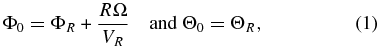
The shape of the individual bundles of magnetic field lines greatly influences solar wind behavior and measuring the FTE profile is a major way to validate magnetic models of the corona. The rate at which magnetic flux tubes expand in a solid angle between the photosphere and source surface (FTE) can be represented mathematically as
where Br(phot) and Br(ss) are the radial components of the magnetic field at the photosphere and the source surface, and R☉ and Rss are the photospheric and source surface radii, respectively. Levine et al. (1977) noted that the magnetic flux tubes with the least expansion corresponded well with the fastest solar wind streams in their study using the PFSS model. Later, Wang & Sheeley (1990) obtained an empirical relationship between SWS and FTE using the PFSS model. This inverse correlation between SWS and FTE implies that both slow and fast solar winds arise from coronal holes and forms the basis of the state-of-the-art solar wind prediction technique—the WSA model (Arge & Pizzo 2000).
We computed FTE at the same heliocentric distance, 2.5 R☉ for both the CSSS and PFSS models, for a meaningful and justifiable comparison. Moreover, it is the FTE in the inner corona that determines the heating rate and the mass flux, and the source surface in the CSSS model is located much farther than that in the PFSS model. The cusp surface is taken as the reference height for the inner corona in this Letter. However, we intend to investigate the optimal height in a future work.
We computed FTEs corresponding to each of the solar wind source locations determined on the source surface, whose photospheric footpoint locations were obtained using the CSSS and PFSS models, and "predicted" the SWS making use of the ranges of SWS and associated FTE (Wang & Sheeley 1990; Wang 1995; Wang et al. 1997). We then obtained a quadratic function (Figure 2) that best fitted the pair of "predicted speed" and the computed FTEs. The coefficients we obtained were a = 110.3, b = −416.0, c = 676.6 and a = 113.9, b = −466.6, c = 763.4, for WSO and NSO data, respectively. This function was later used to predict the SWS using the models. Since the FTEs were computed at the same distance of 2.5 R☉ in both the models we used the same function for the predictions.
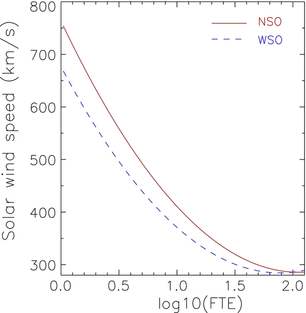
Figure 2. Best-fit function for NSO and WSO data.
Download figure:
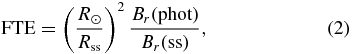
Standard image High-resolution imageWe obtained the root mean square error (RMSE) between the observed and predicted speeds for both models and the ratio (RMSEPFSS/RMSECSSS) between them (RMSE ratio). We also obtained correlation coefficients between the observed and predicted SWSs and a skill score, described by Owens et al. (2005) as

where MSE is the mean square error between the model predicted speed and the observed speed MSEREF is the MSE of the baseline model. Owens et al. (2005) used the MSE averaged over all predictions over a year as the MSEREF, but we, in this Letter, used the PFSS model as reference.
4. RESULTS
Figure 3 depicts the predicted speed using the CSSS (red dashed lines) and PFSS (blue dotted lines) models in comparison with the observed (black solid line) speed mapped back to 2.5 R☉. Panels (a: i—iii) and (b: i–iii) represent the WSO and NSO synoptic maps. In each panel, the CR number, the RMSE ratio between the two models, and the correlation coefficients between the observed and predicted SWS for CSSS (red) and PFSS (blue) are labeled.
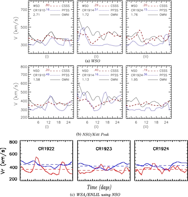
Figure 3. Observed solar wind speed in comparison with speed predicted by the CSSS (red dashed lines) and PFSS (blue dotted lines) models, using WSO (panel (a)) and NSO synoptic maps (panel (b)). The WSA/ENLIL predictions (blue lines) in comparison with observed (OMNI: red lines) solar wind speed is depicted in panel (c); see text for details.
Download figure:
Standard image High-resolution imagePanel (c) in Figure 3 represents the WSA/ENLIL predictions (blue lines) of SWS using NSO synoptic maps, in comparison with in situ data (OMNI: red lines) for Carrington rotations CR 1922–CR 1924 in 1997 (provided by Dr. D. Odstrcil 2013, private communication). The WSA model is built on the PFSS model including a Schatten Current Sheet (Schatten 1971). The predicted SWS is computed using the empirical relationship between the speed and FTE (Owens et al. 2005; McGregor et al. 2008), which includes the angular distance of the footpoint of the field line from the boundary of the nearest coronal hole.
Figure 4 shows the variation of the RMSE with CR for the CSSS (red solid line) and PFSS (blue dashed line) predictions using WSO (panel (a)) and NSO data (panel (b)). The skill scores obtained for the two models using WSO (panel (a)) and NSO (panel (b)) data are shown in Figure 5.

Figure 4. RMSE between solar wind speed observed and predicted: by the CSSS (red solid line) and PFSS (blue broken lines) models, using WSO (panel (a)) and NSO (panel (b)) synoptic maps from 1996–1998.
Download figure:
Standard image High-resolution image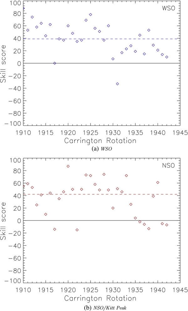
Figure 5. Skill scores (Equation (3)) for WSO (panel (a)) and NSO (panel (b)) data. The horizontal blue and red broken lines represent the average over the entire period of study, 1996–1998.
Download figure:
Standard image High-resolution image
5. DISCUSSION
We compared the SWS predicted by the CSSS and PFSS models, and the near-Earth observations (Figure 3), from 1996 to 1998 (CRs: 1910–1942). The following discussion and our conclusions are mainly based on RMSE in terms of the ratio between the PFSS and CSSS models (RMSE ratio) since we noted that the correlation coefficients between observations and predictions were inadequate to express the performances of the models and the accuracy of the predictions. As generally known, good correlation between two physical quantities need not necessarily imply a causal connection between them, and in the case of forecasting models, it is the accuracy of the prediction that matters. In Figure 3, though correlation coefficients for the PFSS model are larger than that for the CSSS model (panels (a: ii), (b: i and iii)), the RMSE ratio indicates that CSSS predictions are closer to the observed value by a factor ∼2, on average. During the period of study, 24% of CSSS predictions and 15% of PFSS predictions (NSO and WSO data) had a correlation coefficient of 0.5 or more with the observed speed.
The average RMSE ratios were 1.3 and 1.6 using the WSO and NSO synoptic maps. For both WSO and NSO data, 82% had an RMSE ratio ⩾ 1.0, indicating that CSSS predictions are comparable to or better than PFSS predictions. Among these, 55% using NSO data and 32% using WSO data had RMSE ratios > 1.3, which implies that the CSSS model has better predictive capability than the PFSS model. The average RMSE ratio between the WSA/ENLIL and CSSS models was 1.9.
As Figure 4 indicates, on average, the error in the predicted speed increases as the solar cycle progresses toward maximum, suggesting the difficulty in modeling the corona when the global magnetic field becomes complex. This trend is also indicative of the need to better optimize the free parameters of the models for different phases of the solar cycle. For example, we placed the cusp surface and the source surface at 2.5 and 15 R☉. However, it is well known from observations that the height of the cusp point varies over a wide range (e.g., Zhao & Hoeksema 1995; Cranmer et al. 2007). Optimization of these parameters is currently underway.
Referring to Figure 5, the average skill scores over the entire period of study (blue and red broken lines) were comparable, with the CSSS model using NSO data slightly better than that using WSO data. The average correlation coefficient for the CSSS predictions was 0.23, while that for PFSS predictions was 0.12, both using NSO data. The corresponding numbers for WSO data were 0.15 and 0.13. Therefore, overall, the performance, and thus, reliability, of the CSSS model is considerably better using high-resolution NSO data; this is a well-known fact (Arge & Pizzo 2000). For a given synoptic map, our results show that the CSSS model performs nearly 1.5–2 times better than the PFSS and WSA/ENLIL models. Therefore, with the highest resolution synoptic maps from the Helioseismic and Magnetic Imager on board the Solar Dynamics Observatory, the CSSS predictions will be much more accurate.
We infer from Figures 3–5 that for both WSO and NSO data, the error is clearly smaller for the CSSS predictions. That is, taking RMSEs as the metric of accuracy, CSSS predictions are more accurate, by a factor of 1.6, than PFSS and WSA/ENLIL predictions. With the many advantages of the CSSS model (Section 2), which is built on a realistic coronal scenario, our results indicate that the CSSS model is superior to the popular PFSS model.
We, in this Letter, attempted to connect the observed near-Earth solar wind with its source regions on the Sun by mapping them back ballistically and then predicting the speed using the magnetic field properties at the footpoints, represented by FTE. A detailed comparison of the footpoint locations is beyond the scope of this Letter. However, two significant points to be noted here are (1) the observed solar wind was mapped back to a distance of 2.5 R☉ in the PFSS model, as opposed to 15 R☉ in the CSSS model where it avoids the solar wind acceleration region below the Alfvén critical point, a region of great uncertainty. (2) Since magnetic field lines are constrained to be radial at 2.5 R☉ in the PFSS model, the uncertainties in the extrapolated photospheric footpoints can be larger than those obtained using the CSSS model, where magnetic field lines are allowed to be nonradial between 2.5 R☉ and 15 R☉. We interpret the better performance of the CSSS model seen here as a clear indication of the fact that the CSSS model traces solar wind sources at least twice better than the PFSS model or even the WSA/ENLIL model.
We thank Dr. Dusan Odstrcil for providing the WSA/ENLIL results presented here. B.P. wishes to acknowledge Drs. Yi-Ming Wang and J. T. Hoeksema for numerous helpful discussions and Professor P. H. Scherrer for the postdoctoral position at Stanford during which she carried out most of the work. The authors are thankful to the referee for the many helpful suggestions. This work was internally funded by the Southwest Research Institute.