

Abstract
Breath analysis holds the promise of a non-invasive technique for the diagnosis of diverse respiratory conditions including chronic obstructive pulmonary disease (COPD) and lung cancer. Breath contains small metabolites that may be putative biomarkers of these conditions. However, the discovery of reliable biomarkers is a considerable challenge in the presence of both clinical and instrumental confounding factors. Among the latter, instrumental time drifts are highly relevant, as since question the short and long-term validity of predictive models. In this work we present a methodology to counter instrumental drifts using information from interleaved blanks for a case study of GC-MS data from breath samples. The proposed method includes feature filtering, and additive, multiplicative and multivariate drift corrections, the latter being based on component correction. Biomarker discovery was based on genetic algorithms in a filter configuration using Fisher's ratio computed in the partial least squares-discriminant analysis subspace as a figure of merit. Using our protocol, we have been able to find nine peaks that provide a statistically significant area under the ROC curve of 0.75 for COPD discrimination. The method developed has been successfully validated using blind samples in short-term temporal validation. However, the attempt to use this model for patient screening six months later was not successful. This negative result highlights the importance of increasing validation rigor when reporting biomarker discovery results.
Export citation and abstract BibTeX RIS

Original content from this work may be used under the terms of the Creative Commons Attribution 3.0 licence. Any further distribution of this work must maintain attribution to the author(s) and the title of the work, journal citation and DOI.
Introduction
Volatile biomarker discovery is increasingly gaining attention in the improvement of screening, diagnosis, and prognosis in medicine [1]. Volatilome is the volatile fraction of metabolome [2], which contains all those volatile organic compounds (VOCs) generated within an organism. VOCs are organic analytes with a substantial vapor pressure (typically less than 300 Da) and their analysis allows monitoring human chemistry and health related conditions [3]. VOCs reflect metabolic processes that occur in the body and which may change with disease. Thus, finding specific VOC fingerprints that are characteristic of a pathology is an important field of research [4–6]. The analysis of exhaled breath is a specifically attractive and promising means of access to the volatilome, as breath can be obtained non-invasively and contains potentially informative VOCs. VOCs can reach the alveoli, cross the alveolar interface and then be exhaled by the subject [7, 8].
The discovery of new disease markers is based on measuring the global metabolic profile of a sample without bias, which is known as untargeted metabolomics or metabolic fingerprinting [9]. Advanced analytical instrumentation, mainly mass spectrometry (MS) and nuclear magnetic resonance, provides the researchers with possibility of examining hundreds or thousands of metabolites in parallel. Gas chromatography-MS (GC-MS) in particular, is one of the most popular and powerful analytical techniques for breath analysis [8].
The comparison of metabolic fingerprints among different experimental groups; namely condition and control, can lead to the identification of metabolic patterns that have changed due to a disease, and which may be used as a diagnostic tool. Chemometric or pattern recognition methods are required to extract information from exhaled breath data and discover relevant VOCs [10]. However, many data processing techniques are not designed to deal with large amounts of irrelevant or correlated features, which is the case with current analytical technologies that are applied to metabolomics. For instance, in a review on the statistical analysis of metabolomics data, Vinaixa [11] observes a number of metabolomics studies (based on liquid chromatography-MS, LC-MS) where the number of features ranges between 4000 and 10 000, while the number of subjects is always below 30. In other words, from a data-analysis perspective, metabolomics data is characterized by high dimensionality and small sample counts. Consequently, the 'Curse of Dimensionality' [12] has to be taken into account, and data processing methods must be scrutinized in their ability to deal with small sample-to-dimensionality ratios [13, 14]. The inherent difficulty in the analysis of this type of data has long-been recognized and methods to deal with it have been proposed since the 60s [15]. The application of conventional statistical testing is plagued with theoretical difficulties [16], and in many cases machine learning approaches are preferred. However, the scarcity of examples poses problems with respect to the complexity of those predictive models that may be built. Complexity control can be attained through regularization or through dimensionality-reduction techniques [13]. Some authors advocate the use of penalized likelihood estimation [17]. One example is the use of the least absolute shrinkage and selection operator based on L1 penalty in the quest for sparse solutions [18], while others propose projection methods, such as principal component analysis (PCA) [19] or partial least squares-discriminant analysis (PLS-DA) [20]. However, the use of feature selection methods based on iterative searches and optimization procedures, using either wrappers or filters as objective functions is perhaps the most popular approach [21]. The performance of these methods in high-dimensionality, small-sample conditions has been analyzed previously [22]. Among them, genetic algorithms (GA) have been used extensively [23–25]. The combination of GA and PLS-DA in metabolomics has been previously reported [26].
The application of dimensionality-reduction techniques based on feature selection methods is therefore the natural choice [17].
Breath analysis is particularly challenging due to the lack of standards for sampling and storage that are employed [27–29]. As such, researchers prefer to analyze breath samples soon after collection. If patient recruitment takes a long time, then analysis may extend over several months. In these conditions, instrumental changes, such as chromatographic column aging, temperature variations and the effects of contamination can shift intensity value measurements over time [30–33]. As computational methods in metabolomics rely on a quantitative comparison between metabolite abundances in diverse groups, instrumental drift may become an important source of errors. It is therefore extremely important to block this potentially confounding factor at the design stage, if possible [34]. Another inherent difficulty involved in breath analysis is the large inter and intra-individual variability of exhaled breath, even among healthy subjects [35], and the change of VOCs patterns according to food consumption, smoking, gender, age, and so forth [36, 37]. There are definitely several sources of unwanted variance that may act as confounding factors, and which can be divided into two types: instrumental (e.g. different location, operator, instrument or sampling conditions), and clinical (e.g. gender, age, smoking status, comorbidities or treatments) [29, 38]. If some factors cannot be controlled with experimental design [39], they must be taken into consideration during data analysis [40].
Normalization methods adjust data for biases caused by non-biological conditions or unwanted variations [36, 41, 42]. Most adopted normalization methods rely on scaling factors using all the data set (e.g. total sum or norm). However, these methods have been shown to adjust data incorrectly, as an increased abundance in some metabolites leads to a decrease in other metabolites [43].
Alternatively, internal standards (IS) and quality control (QC) samples are often used for the posterior removal of certain systematic errors that maybe platform specific [40]. The IS method is based on the addition of known metabolites (in a determined amount) to the samples in order to improve quantitative analysis and normalize each sample according to their variation. The simplest approach is based on a single IS and assumes that the variation in sensitivity observed for this metabolite is constant across all the analytes. Thus, a multiplicative correction factor may be applied. However, it is not clear that the underlying hypothesis can be sustained, and therefore the use of multiple IS has been proposed, but then the selection of the proper normalization method remains an open problem. Application examples of normalization methods based on IS have been reported on literature [40, 43]. For instance Sysi-Aho et al proposes that the correction factors are a linear function of the variation observed for the IS, and he optimizes the coefficients of the model to maximize the likelihood of the observed data [32]. However, in untargeted studies, the metabolites that are to be detected are not known a priori, and therefore the addition of numerous IS for detection and to normalize for analytical variation is not practical, indeed it would prejudice the integrity of the samples [31]. As such, QC are often preferred in untargeted metabolomics in order to avoid changing the physical sample and using IS that may coelute with metabolites of interest [44]. QC samples may be either commercial or pooled (i.e., a mixture of equal aliquots from a representative set of the study samples). The latter are of special interest, as their measurement contains all those metabolites under investigation. Even though pooled QC samples may be relatively easy to prepare for some biofluids, such as urine or plasma [45, 46], exhaled breath presents inherent complications in terms of sampling and storage, which prevents its use, especially in long-term studies. Different signal correction methods rely on QC samples [44, 47], which can be employed to estimate sample- or feature-based correction factors [31]. According to previous works [42, 48], one of the best normalization methods that employs QC samples is probabilistic quotient normalization (PQN) [49].
Since machine drifts are frequently observed in chromatography and MS, the assessment of reproducibility and repeatability is of utmost importance [50, 51]. Over the last decade, a number of computational algorithms have been applied in order to correct instrumental drifts, or batches in data. For instance, ComBat technique was proposed in the genomics field and was later also applied in metabolomics, for adjusting data for batch effects [30, 52]. Many methods are based on projection filters. Examples of these methods are component correction (CC) and common PCA (CPCA). They consist of the estimation of the drift subspace with a reference class or the entire data set, respectively, and the subtraction of this subspace from the original data [30, 53]. The dimensionality of the drift subspace should be carefully determined using calibration data, in order to avoid valuable information removal. For example, Fernández-Albert et al used Dunn and Silhouette indexes to compare different drift correction methods and the dimensionalities of the drift subspace [30]. Another example in this family is orthogonal signal correction, which removes the data variance that is uncorrelated to the class information [54]. Similarly, orthogonal projections to latent structures, such as orthogonal PLS algorithms, have also been applied for drift compensation [55–57]. The existing literature mostly uses these methods for predictive models, but not specifically in biomarker discovery, where the impact of instrumental drift on computational biomarker discovery is not yet totally understood, and remains an under-studied topic.
Unfortunately, those studies of biomarker discovery in metabolomics that have been undertaken are usually plagued by statistical bias, and involve small sample sizes, which lead to very poor reproducibility. This is aggravated by the use of weak validation methodologies that mostly consist of internal validation. We believe that only external validation (blind samples) can provide further reliability to biomarker discoveries. Moreover, an additional temporal validation, undertaken months after the model development process has been closed, should be a recommended practise. However, in most published literature this long-term validation is missing. If we expect that discovered biomarkers can be adapted and be put into clinical use, then their use has to be reliable enough to maintain predictive power in a variety of instrumental conditions, or even instrument vendors. Reporting long-term validation results would allow the discovery of the limitations of current research and speed up further investigation into the most promising biomarker discovery studies.
In this work, methods for the instrumental drift in GC-MS data from exhaled breath are proposed and investigated through their application in a practical case. The analyzed dataset consists of breath samples obtained from patients with lung cancer (LC), chronic obstructive pulmonary disease (COPD), and control subjects, in order to discover the markers of these diseases. Since this dataset was acquired over a two-year period, the correction of instrumental drift in the entire dataset was one of the data analysis objectives. The influence of time varying effects requires special attention to the application of strict validation procedures, which was an essential part of our workflow. We not only used external validation, but also an additional temporal validation in order to assess the predictive power of the biomarkers, six months after the end of the model development phase, which is a validation level that is not usually reported in similar studies. From a machine-learning standpoint, biomarker discovery may be addressed using feature-selection techniques.
In this quest for putative biomarkers, additional issues, such as potential clinical confounders have also been investigated. Finally, biomarker selection and classification was applied to the binary problem case of COPD versus control.
Experimental methods
Sampling system
Exhaled breath was collected using the tidal breath sampler shown in figure 1, which was and developed by the Department of Biochemistry and Molecular Biology of the University of Barcelona [58]. It consists of a glass tube with a specific shape that allows the collection of tidal exhaled air. The subject breathes into a unidirectional Rudolph valve, which allows medical air (22% O2, 78% N2) contained in a Douglas bag to pass through his mouth and which then transports the exhaled breath to the glass tube. An air pump (FLEX Air Pump 1001) extracts the air from the first section of the glass tube and drives it to a sorbent trap that is filled by a fiber comprising 200 mg Tenax and 200 mg Unicarb. Between the glass tube and the fiber is a filter made of silica gel, to avoid humidity, which distorts mass spectra. In order to avoid breath condensation on the walls of the glass, the tube is heated using a long, warmed filament, which is wrapped along its length. See supplementary material is available online at stacks.iop.org/JBR/12/036007/mmedia for sampling protocol information.
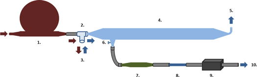
Figure 1. Tidal breath sampler. A diagram of the sampling system used to collect VOCs from exhaled breath is shown above. 1: Douglas bag with medical air. 2: Unidirectional Rudolph valve. 3: Mouthpiece for subject's breath. 4: Glass tube at high temperature. 5: Outlet for the vast majority of air. 6: Outlet for the final part of the subject's exhalation (containing the VOCs from gas exchange). 7: Silica gel filter for humidity control. 8: Sorbent trap. 9: Air pump. 10: Air exiting the pump.
Download figure:
Standard image High-resolution imageGC-MS analysis
Samples were injected into the gas chromatograph system using a Unity thermal desorption unit for sorbent tubes (Markes). This unit applied a flow of hot carrier gas through the fibers contained in the sorbent traps, desorbing the VOCs in its surface and carrying them to the GC system (FocusGC, fThermo Scientific). The chromatographic column used was a 60 m DB-624 capillary column with an internal diameter of 0.32 mm and a stationary phase thickness of 1.8 μm. The temperature ramp used to optimize the separation and sensitivity of the chromatographic process was: 40 °C (5 min)—10 °C (1 min)—180 °C (1 min)—15 °C (1 min)—230 °C (10 min). Once eluded from the column at different retention times (RTs), the separated compounds were injected into the MS (DSQII MS, from ThermoScientific), where they were ionized via electron impact and subsequently fragmented. In order to reuse the sorbent traps, once desorbed, they were then cleaned to eliminate any possible remaining VOCs, with a flow of N2 at 320 °C for 2 h, before being closed and stored in vacuum.
Dataset and data processing algorithms
Dataset description
The dataset contained four classes or medical groups: control, COPD, LC, and both diseases (COPDLC). Standard diagnostic criteria were used for the inclusion of each study group. The main exclusion criteria were: (i) Lack of clinical stability; (ii) Abnormal non-obstructive forced spirometry results; (iii) Previous history of cancer; (iv) Previous history of active inflammatory disease; (v) Treatment with steroids or immunomodulators; and, (vi) Data suggesting infectious disease. The protocol was submitted and approved by the Human Studies Ethical Committee at Hospital Clinic and all patients signed informed consent forms before any procedure was initiated.
The sample collection procedure lasted almost two years (from 20/5/11 to 6/5/13) and was divided in two campaigns. The first campaign lasted from 20/5/11 to 7/3/12 and was divided into calibration (initial 80%) and short-term external validation set (last 20% of each class). The second campaign lasted from 10/7/12 to 6/5/13. It is important to note that the collection and analysis protocol was identical in both campaigns. The purpose of the second campaign was to further validate the results obtained from the study carried out in the first campaign. This second campaign served not only to provide blind samples, but also to test the stability of the predictive model. It is important to note that this stability test is neglected in most studies and validation is internal to the same measurement campaign. All model development and optimization, including drift counteraction strategies, was undertaken within the calibration set. The number of samples included in the study is summarized in table 1.
Table 1. Data set overview. The number of samples of each class is reported by data subsets (calibration, short-term, and long-term validation) and also the total number. COPD: chronic obstructive pulmonary disease, LC: lung cancer, COPDLC: COPD and LC.
| Data subsets | Control | COPD | COPDLC | LC |
|---|---|---|---|---|
| Calibration | 15 | 22 | 15 | 10 |
| Short-term validation | 6 | 7 | 4 | 2 |
| Long-term validation | 6 | 5 | 5 | — |
| Total | 27 | 34 | 24 | 12 |
The metadata of the patients was also available, including sex, age, weight, height, smoking status, functional respiratory results (forced expiratory volume and forced vital capacity) and haematology tests, current treatments or drugs that the patients were taking, comorbidities (e.g. hypertension, asthma, diabetes), and diagnostics of the studied disease.
Apart from the patient samples, two types of spectra blanks were available: (i) 7 fiber blanks (GC-MS analysis of new sorbent traps that were not previously used for any sample), and (ii) 49 sample blanks (GC-MS analysis of sorbent traps in each day of measurement). Fiber blanks are used to assess the existence of specific peaks due to the presence of fiber, whereas sample blanks serve to assess the potential contamination of the system. Even if no sample is injected, a signal can be obtained, due to the VOCs trapped in the column, while sample blanks provide quantification.
Data pre-processing
Data pre-processing was performed with MZmine2 [59] software. Peak detection was based on the Noise Amplitude algorithm. In this algorithm, intensity range is specified by the user and the algorithm automatically locates the where the noisy baseline is concentrated, and establishes the baseline level at this level. A peak is recognized when the chromatographic signal is registered above the noise level during a certain time span. A smoothed second derivative, Savitzky–Golay digital filter is then used to detect the borders of the peaks. After detection, peaks were aligned using the RANSAC aligner. Here the RT tolerance was 1 min, with an m/z tolerance of 0.4. The number of iterations was automatically determined by the software. MZmine also provides tools for isotopic peak grouping and gap filling in the event of missing values [60]. After MZmine pre-processing, 3049 peaks with an associated intensity were obtained. Each peak was identified by its mass to charge ratio (m/z) and RT. The area under the peaks was computed in order to obtain the data matrix. Since there were peaks with the same RT (differences less than the GC resolution, 0.1 min) and large correlation (Pearson correlation r >0.9) between them, they were considered to be part of the same original compounds. By clustering these peaks and removing near zero variance features, the dimensionality of the data was reduced from 3049 to 1749 features. In total, 1297 features were removed by peak clustering, while 3 were removed, as they had near zero variance. Finally, 1793 features (peak areas) were retained.
Rank products
Rank products (RP) is a feature-selection algorithm proposed by Breitling that is used to find the differentially expressed genes [61]. It is an intuitive method that was designed to rank genes according to the up or down-regulation magnitude in all microarray replicates. If one variable is highly ranked in many replicates, greater confidence can be given to the consistence of the results. The RP method has been widely applied in other domains, such as proteomics and metabolomics [62, 63]. RP provides an estimator that may be computed for each feature. It is important to compare the obtained RP value with the sampling distribution under the null hypothesis that the differential expression values are identically distributed. In order to do this, we have used the permutation sampling procedure originally proposed by Breitling, using 100 iterations. In order to calculate the RP estimator, the RankProd library in R was used [64]. For each feature f in k replicates, each containing ni features, the RP is calculated as:

where  is the ranking position of the feature f in the replicate i.
Probabilistic quotient normalization
PQN method estimates a gain for every sample by using a reference spectrum [42, 49]. This reference spectrum is normally a QC sample made up of a pooled mix of equal aliquots from a representative set of the study samples. The median of the ratio between the sample and reference spectrum is computed and serves as a quotient to compensate for variations.
for sample i with features xi,j—with j ranging from 1 to n. xiPQN is the corrected feature vector for sample i and xref is the reference spectrum with features xref,j. Note that the median is calculated across samples for each feature. The challenges associated with normalization techniques in metabolomics are discussed by Filzmoser [42].
Component correction
CC assumes that the variance introduced by the drift is explained with one or more principal components (PCs) of a given reference class [30]. PCs that define the drift subspace are subtracted from the original data [54].

where Xc is the corrected data, X is the original data matrix, and P are the loadings (or PCs) spanning the drift subspace.
Genetic algorithms
GA are a feature-selection technique based on the survival of the fittest individual [65]. An individual is defined as a subset of selected features (binary vector with 1 and 0 s, which are taken to mean selected or not selected, respectively). GA initializes a population of many individuals and evaluates their performance according to a predefined criterion (fitness function). The fittest individuals are selected and used to generate a new population through crossover; either by mating and/or by mutation. The chosen figure of merit has been the generalized Fisher ratio [66], computed in latent variable (LV) space using internal validation samples. This goal function is more sensitive than the classification rate (CR), and it is known that filters are less computationally expensive than wrappers.
The general framework was obtained from GA library [67]. Readers interested in an overview of feature selection techniques for omics readers are referred to Gromski et al [68] and Saeys et al [21] and the examples therein.
Partial least squares-discriminant analysis
PLS-DA can be understood as a PLS regression between a data matrix, X, and a categorical one, Y [69, 70]. X contains the set of predictors, whereas Y consists of labels or responses, in this case a binary vector. PLS regression is based on an iterative process to define a new subspace of LV [71]. In order to define it, PLS considers a compromise between maximum variance modeling X and maximum correlation with Y. Different algorithms are used to compute PLS, in this work, the kernel PLS algorithm implemented in pls R package has been applied [72]. The use of PLS-DA for metabolomics has been covered extensively in the literature [73, 74].
Random forests
Random forests (RF) [75] are machine-learning techniques often used for omics data analysis for the purposes of classification [76]. RF is an ensemble classifier that consists of multiple decision trees, each of which is built using a subset of features and data samples. They also possess an additional advantage in that they deliver an automatic ranking of variable importance that can be used for biomarker discovery [77]. Here the RandomForest R package was used.
Data analysis protocol
Instrumental drift correction
Data was inspected by PCA in order to determine the effect of time. Blanks were then used for in order to filter out noisy features. To this end, two strategies were adopted: (i) Non-parametric Wilcoxon test for fiber blanks, and (ii) RP for sample blanks. The one-sided Wilcoxon test [78] was used to check which features had a median distribution of intensity values that were higher in sample than in fiber blanks. Metabolites that were equally or less abundant in sample than in fiber blanks were considered as contamination, as they were likely to be non-informative, and as a result, they were discarded. The testing of this hypothesis was performed for all classes taken together, versus fiber blanks, due to the availability of only 7 fiber blanks. The RP method, however, was applied in order to compare the metabolic profiles of each class versus the sample blanks, for which a larger sample of 49 blanks was available. Therefore, four contrasts were defined in order to assess which features possessed more intensity in any of the classes than in sample blanks. The consideration of all samples (control, COPD, COPD-LC, and LC) in the same group in order to undertake the contrast versus sample blanks may have resulted in peaks that were highly abundant only in one class being removed. Thus, in order to avoid removing the relevant variables, all those variables that were more present in any patient group than in blanks were retained.
Contamination and memory effects in the conserved ion fragments were assumed to be additive noise that could be corrected. The intensity measured in the previous blank was then subtracted from the intensity of an ion fragment from a sample [79, 80]. The possibility of gain variations in time was explored beyond the additional correction of potential instrument contamination. A normalization strategy inspired in PQN was introduced, which was aimed at removing the so-called size-effect [42]. The major difference between PQN and the applied method is that the gain variations were estimated with sample blanks. The multiplicative factor of a sample is given by the median of the ratio between the reference blank and a blank acquired previous to sampling. The reference blank chosen was one of 13/12/11, as intensity fluctuations within that time period were limited. The expression that encompasses both the removal of sample blanks and multiplicative correction is the following.

where xi is a sample, xiC is the corrected sample, xBlank i is the previous blank to the sample, and xBlank ref is the blank of reference in the middle of the study (13/11/11).
Moreover, CC was applied using sample blanks as the reference class to estimate drift subspace. Two figures of merit were considered at this stage, in order to optimize the number of PCs to be eliminated: the Pearson Correlation Coefficient of data with time [81], and the Hotelling T2 Statistic, which is used to estimate the distance between classes [82].
Potential clinical confounders
Then hypothesis testing was used to check if controlled clinical variables were equally distributed between the defined groups, or if they acted as confounding factors. Tests were carried out to compare classes two-by-two. The Chi-squared test (or Fisher's Test, if at least one expected frequency was lower than 5) was applied to the factorial variables; sex, smoking status, presence of hypertension, and presence of diabetes [83]. For the numerical variables; age and body mass index (BMI), the non-parametric Wilcoxon Test was used.
Biomarker discovery
Pre-processing included outlier detection using the Mahalanobis distance, centering and auto-scaling to unit variance. Biomarker candidates were selected by GA, Fisher's ratio computed in PLS-DA LV space being the figure of merit to maximize [84]. Some measures were adopted following the recommendations of Leardi and Lupiáñez González to ensure a proper choice of selected features that do not lead to model overfitting [85]. One of them was to limit the number of GA iterations according to the fitness saturation of the best individual. Moreover, in order to avoid the exploration of only a reduced part of the search domain, different GA runs with random initialization were performed, and feature selection frequencies were computed. The entropy of this feature selection frequency distribution was introduced as a stopping criterion for GA [13]. The saturation of entropy was related to a stable feature selection that does not change with more runs, i.e., more executions do not lead to an increase in information. The frequency distribution of a random selection (simulation of random selection 1000 times) was computed, and the final subset consisted of those features selected in more runs than would be expected by chance. A PLS-DA model was built with this feature subset, and the number of LV was optimized using a cross-validation in the calibration set. External validation of the model was carried out using short-term and long-term validation data, and permutation tests of 10 000 iterations were employed to check if the results were statistically significant as compared to a random classification.
At this point it is important to note that the data processing workflow implemented that includes feature selection using GA provides only fragment candidates. Mass spectra matching is needed to obtain analytes from fragment candidates. The NIST Mass Spectral Search Program 2.3 was used for this purpose.
For reasons of comparison, the use of feature selection based on PLS-DA and RF models was also explored and compared to the proposed methodology of GA and PLS-DA. On the one hand, the variable importance in projection (VIP) was applied to the global PLS-DA model (without GA) [86]. Moreover, two variable importance measures were used for the RF model. The first was the total decrease in node impurities from splitting on the variable, averaged over all trees (for classification, the Gini index). The second measure of importance was based on the error rate in classification for out-of-bag data, when variable predictors are permuted and averaged over all trees.
Results and discussion
Instrumental drift correction
Data inspection: unsupervised exploration of time effects in uncorrected data
For a better understanding of high dimensional data, it is convenient to visually inspect the projection to subspace that capture maximum variance using PCA. Figure 2 shows PCA score plots for calibration and short-term validation subsets. Figure 2(a) is colored according to date of acquisition and reveals a clear relationship between the maximum variance directions in the data set and time. The two observed clusters are not due to the medical conditions under study, as it can be seen from figure 2(b), but consist of unwanted variance that should be removed, since it seems to be causing a separation between samples collected at various times. Therefore, through unsupervised data exploration, an instrumental signal drift explaining a considerable variance of the dataset was detected. However, it was not possible to specify a particular date in which the instrument changed within the calibration subset.

Figure 2. PCA score plot of calibration data. Score plots of PC1 and PC2 are shown (a) coloring samples (using a two-color gradient) according to the date of acquisition (i.e., number of days since the first data acquisition of the study), and (b) coloring samples according to the class under study.
Download figure:
Standard image High-resolution imageFeature filtering
In this section, we set up procedures to select features that are informative about the breath composition of the subjects, while rejecting sample contamination due to the absorbent fiber used or memory effects in the instrument. In order to do so, we took advantage of the two types of blanks were available in this study, fiber and sample blanks. They provide a measurement of baseline noise due to peaks caused respectively by the fiber or memory in the instrument in each day of acquisition. These data were employed to reduce the dimensionality of the dataset by removing noisy features. We would like to emphasize that this feature filtering (FF) was exclusively done using calibration data.
First, a univariate Wilcoxon test indicated that 1693 of 1752 features had significantly higher intensity profile in patients' samples than in the analysis of fiber blanks (new sorbent traps without samples). For the rest, the null hypothesis was accepted, and 59 features were removed from the data. In this step, features that fulfilled the null hypothesis were filtered out. With the intention of removing only those features that clearly belong to the blanks, no multiple testing correction was implemented. Multiple correction testing is stricter in order to identify samples that do not conform to the null hypothesis but, in this case, the aim was to identify features that clearly do conform to the null hypothesis.
Second, an alternative use of the RP method, which is often utilized as a univariate feature selection for biomarker discovery in genomics, was proposed. Instead of comparing classes under study among them to find putative biomarkers, binary contrasts of each class versus sample blanks were computed. Features can have larger value distributions in one or more classes with respect to sample blanks, and RP results indicated that 79 features had higher intensity in one study class, 66 in two, 84 in three, and 243 in the four classes with respect to blanks. With this RP strategy, dimensionality was further reduced, from 1693 to 472 features. Figure 3 shows that eliminated features mainly correspond to compounds eluting at longer RTs, which might be related to compounds of lower volatility, higher molecular weight, or more affinity with the chromatographic column. Since these RTs were shown to contribute more in the PCA loadings of the initial data, they largely hide the effect of lower intensity features. As a consequence, FF did not only reduce computational cost, but probably improved the power in identifying real biomarkers.
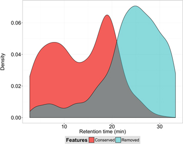
Figure 3. Data filtering based on sample blanks data. Density estimations are shown for the retention times of the conserved (red) and removed (blue) features using sample blanks data.
Download figure:
Standard image High-resolution imageThe score plot in figure 4 indicates that despite this filtering, the data still showed a temporal separation of samples. In this figure, long-term validation samples were also added to show how they differ from the other data points. When the long-term validation subset is considered, the first PC reflects the separation between them and the rest of samples, and the second PC is the one which reveals the two previously observed clusters.

Figure 4. PCA score plot of all the data of the study after filtering. Score plots of PC1 and PC2 for all the samples (calibration, short-term, and long-term blinds) after data filtering using blanks data (i.e., data set with 472 features).
Download figure:
Standard image High-resolution imageFigure 5 represents the first PC scores with respect to the date of acquisition and also shows that long-term data are remarkably different from the samples collected during the first year of the study. Acquisition of the last data subset was over a long period of time, which results in different batches even within long-term validation samples.
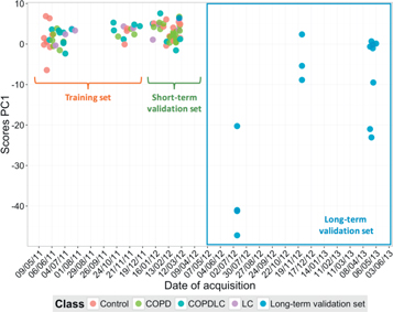
Figure 5. Change of PC1 scores over time. Score plots of PC1 are reported for all the samples with respect to the date of acquisition for filtered data (i.e., 472 features).
Download figure:
Standard image High-resolution imageEven though in this study there were no QC samples, inspection of the changes in sample blanks allowed us to learn about time effects. Our initial observation was that sample blanks shared a lot of common fragments. On this basis, additive and multiplicative corrections were proposed.
Additive and multiplicative corrections
We have already mentioned that ion fragments with the same amplitude in the real samples and in the blanks were discarded. Beyond this additive correction, sample blanks showed contamination and memory effects in the conserved features. Therefore, each sample had the intensity values of the previous blank subtracted from its intensities. Even after additive correction, large variations in the intensity of the chromatograms were still observed and the possibility of gain variations over time was explored. Figure 6 shows boxplots of the intensity ratios between a reference blank in the middle of the study and the rest. While ratios among fragments showed some scatter, there was a clear central value that differed across days. This effect leads us to the hypothesis of instabilities of sensitivity over time. In order to compensate for this, a gain correction was estimated through the median of the ratios across ion fragments. Figure 6 reports a clear pattern for a change in the gain over time. There was a sharp variation in the gain on a particular date (10/07/12), which separates the group of the short-term and long-term validation data.
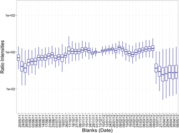
Figure 6. Intensity ratios of sample blanks. The ratios between a reference blank (13/12/11) and the rest of the blanks are shown for each date of acquisition. Note that the time scale in the x-axis is not uniform.
Download figure:
Standard image High-resolution imageIn order to compensate for the observed time effect, the multiplicative correction method described by equation (4) was used—this assumes that there is a uniform gain variation across features for each sample. Additionally, an underlying hypothesis for this correction is that the estimated gain variation with sample blanks is the same for all the samples measured in this particular day. This normalization approach to correct the multiplicative effect is inspired by PQN, but using data from blanks as reference.
The application of the former normalization method minimized the effect of gain variations, and the long-term validation data was especially effective in diminishing their variability with respect to the rest of samples. However, temporal variation might also be correlated among features and, consequently, some privileged drift directions may exit. To account for such multivariate correction of instrumental drift, CC was implemented.
Component correction
For CC, sample blanks were chosen as the reference class. Variance in the reference class was modeled with PCA. The technique assumes that the drift subspace was shared between the blanks and the samples. This drift subspace is spanned by a number of PCs estimated from the PCA of the blanks. Since the removed component(s) might be explaining not merely the drift, but also biological differences under study, it is important to optimize the number of removed components and making an appropriate trade-off is essential. Correlation of data with time decreased with respect to the original data when removing the first PCs of sample blanks, so CC appeared to diminish the temporal dependence. Moreover, the use of the two-sample Hotelling T2 statistic was proposed to estimate distance between classes. Results showed that removing the first PC of the blanks in the original data matrix maximizes the Hotelling T2 statistic. Therefore, one PC was shown to minimize correlation with time and maximize distance between groups in binary contrasts (as measured by the Hotelling statistic).
Figure 7 shows the PCA score plot for data corrected by the methodology we have outlined. The two 'date of acquisition' data clusters vanished after the correction was applied. In addition, long-term validation samples are closer to the other data points. Visually there has been a great improvement, but the correlation of the data with time was also computed to compare the methods, in particular the four cases explained above i.e. FF, FF plus additive and multiplicative correction (AM), feature filtering plus CC, and the combination of all the methods (FF + AM + CC).

Figure 7. PCA score plot of all data after multiplicative and component correction. Score plots of PC1 and PC2 are reported after multiplicative and component correction based on sample blanks data.
Download figure:
Standard image High-resolution imageFigure 8 shows that correlation with time substantially diminished when applying the three strategies: FF, additive and multiplicative correction, and CC. Therefore, blanks were successfully used to diminish the significant instrumental drift present in the GC-MS data.

Figure 8. Comparison of applied corrections. The correlation with time (r coefficient) is shown for original data (O), data after feature filtering (FF), FF plus additive and multiplicative corrections (AM), FF plus component correction (CC), and the combination of the three strategies, FF + AM + CC.
Download figure:
Standard image High-resolution imagePotential clinical confounders
The clinical variables, sex, age, BMI, smoking status, and the two more frequent comorbidities in the dataset, hypertension and diabetes mellitus II, were tested for different distributions between study groups. These factors were equally distributed between the study groups COPD and control (with 95% confidence). However, there were potential confounding factors for the cases of COPDLC (hypertension, age, and smoking status) and LC (hypertension).
Biomarker discovery
LC and COPD are complex diseases; indeed, both are a family of condition subtypes and COPD can be an indirect warning of LC. Hence, identification of VOCs signatures which allow proper classification of all condition subtypes is a real challenge, especially with insufficient data. Additionally, the consideration of clinical confounders in the final model complicates biomarker discovery even further. Due to these difficulties, the present study has corrected instrumental drift for the complete data set, but has focused on the case of COPD for the biomarker discovery stage. COPD intensity profiles were compared with those of the control group. This is the condition-control binary classification problem but with more samples available (15 for control, after eliminating 3 outliers, and 23 for COPD in the calibration set), and clinical confounders were not found.
Biomarker selection
Our biomarker selection strategy aimed at finding a small subset of features that may discriminate the two classes, in contrast to other strategies that identify volatile fingerprints with several tens or even hundreds of compounds. The discrimination of disease by a small subset of variables opens the possibility of further development of specific sensor kits for point of care, or clinical applications after biomarker identification.
The search technique based on GA looked for the features that maximize the distance between the classes in the PLS-DA subspace. The selection reached the entropy saturation criterion after 35 GA runs. Figure 9 reports the frequency of selection of the features after these 35 runs. The hypothesis of this approach is that combinations of features that exhibit random correlations tend to be selected less often than real discriminant features after some trials. Figure 9 shows that nine features were systematically chosen by the algorithm. Hence, they were assumed to contain class discriminant information and constituted the subset of putative biomarkers.
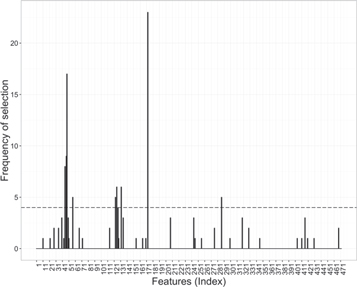
Figure 9. GA selection. Frequency of selection for every feature after 35 runs of the GA. Features above the threshold were ultimately selected, while features below the threshold were selected as often as would be expected at a random.
Download figure:
Standard image High-resolution imageMetabolite identification
As we have already mentioned, the methodology implemented provides only fragments, or groups of fragments, that are characterized by an RT and a, m/z. To identify the metabolites, the correlation threshold for fragment grouping, which initially was set to 0.9, was decreased. By decreasing this threshold to 0.6 for fragments appearing at the same RT (with a window of 12 s), more complete mass spectra were obtained, which allowed the identification of three putative biomarkers. A fourth set of fragments did not match any candidate compound from the NIST library.
- (i)Isoprene. This compound appears both in healthy and COPD subjects. Isoprene is a major metabolite in the breath. It has been mentioned as a product of lipid peroxidation and previous studies have linked it to cholesterol metabolism [87]. This compound has been proposed as biomarker for COPD in previous studies [5] and has been detected in breath associated with other respiratory diseases [88], including lung cancer [89]. The utility of isoprene as biomarker has been reviewed by Salerno-Kennedy and Cashman [90].
- (ii)Succinic Acid (Succinate). Succinate in living organism has many roles as a metabolic intermediate and as a signal of metabolic state at the cellular level [91]. It is generated in the mitochondria through the Krebs cycle. Succinate has been proposed as a metabolic signal for inflammation [92], and has been found at an increased level in inflammatory bowel disease and colitis [92].
- (iii)Pentamethylene sulphide. This compound appears in diverse patents as related to medication of COPD as a chymase inhibitor [93, 94] and also in the formulation of anti-inflammatory agents [95]. Consequently, we suspect that this is not a biogenic compound, and may be related to the patients' medication.
The ranking of fragments provided by VIP in PLS-DA global model, and the feature importance provided by RF, were also compared. We note that the models were much less sparse than the ones obtained after our GA feature selection. Particularly for VIP in PLS-DA, there were many fragments providing similar values. There was not a good matching between the fragments selected by GA, and the ones ranked higher in VIP. On the other hand, RF gave a very high (top five positions) ranking to fragments related to Isoprene, but the rest of fragments selected by GA were medium-ranked by RF.
Predictive modeling: assessment of accuracy in short-term external validation
Calibration data were used to assess model complexity assessment, both feature selection and optimization of the number of LV. Internal cross-validation determined that LV = 2 was the optimum hyperparameter for a PLS-DA classifier with the selected features. A final PLS-DA model was built with all the calibration data, in order to estimate its predictive performance when classifying new samples as control or COPD.
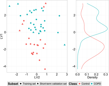
Figure 10 shows the PLS-DA score plot for control and COPD classification, including calibration and short-term validation subsets. Control and COPD groups have distributions that are slightly separated. The first LV gives two density distributions with a certain overlap and the inclusion of the second LV in the model provides a small increment in the distance between classes. For short-term validation data, the model correctly classified 77% of the samples (CR = 77%) and had an area under the ROC curve (AUC) of 0.75. Sensitivity was 100%, i.e., all patients with the disease had a positive result, whereas the specificity was lower, 50%. Obviously, the trade-off between sensitivity and specificity can be adjusted by proper selection of the classifier output threshold. Moreover, permutation tests for CR and AUC distributions gave p-values of 0.015 and 0.029, respectively, which are statistically significant.
Figure 10. PLS-DA scores. LV1 and LV2 scores for calibration and short-term validation data subsets of control and COPD groups are reported.
Download figure:
Standard image High-resolution image
Results were compared to other standard classifiers in metabolomics, namely: (i) PLS-DA on the corrected data without any feature selection using GA and (ii) RF. For PLS-DA, internal validation provided a model with five LVs with a classification in the short-term external validation which resulted in an accuracy of CR = 0.73 ± 0.13 and an AUC = 0.74. Maximum accuracy resulted in a sensitivity of 100%, but a poor specificity of 33%. For RF, the same level of accuracy CR = 0.69 ± 0.13 was reached, but with a poorer AUC of 0.60. These results were achieved with an optimum number of variables (mtry in the RandomForest Package) of 25.
Table 2 shows that all models show a moderate prediction capability, despite the drift in the dataset. However, there is clear evidence that, after feature selection, the PLS-DA model achieves a higher accuracy, and has the added advantage of providing parsimonious models involving a reduced number of biomarkers.
Table 2. Predictive model performance in short-term external validation.
| Model | CR | Sensitivity | Specificity | AUC |
|---|---|---|---|---|
| PLS-DA with GA | 77% ± 12% | 100% | 50% | 0.75 |
| Random forest | 69% ± 13% | 100% | 33% | 0.60 |
| PLS-DA | 73% ± 13% | 100% | 40% | 0.70 |
Predictive modeling: assessment of accuracy in long-term external validation
One of the objectives of the present investigation is to improve the validation of the predictive models, and the biomarkers involved in the prediction of the subject conditions. Unfortunately, most published works disregard this step, and present the results with internal validation or external validation data extracted from the same measurement regime. When these external validation data (blind samples), are time interleaved with calibration samples, the time effects do not play a role since, the model 'knows' about the future changes in the dataset. However, in the quest for the maximum reliability of the chosen biomarkers, the predictive models should, in the future, be able to deliver accurate classification of the calibration. In other words, the model should be resilient to instrumental or operator changes.
Results for the long-term validation of the PLS-DA model with the selected biomarkers were equivalent to a random classification (CR = 55% with a p-value of 0.726). Therefore, the built model had a certain degree of predictive ability in the near future, but this did not hold for samples acquired during the second year of the study. Instrumental signal drift caused considerable changes on intensity profiles, chiefly during long-term validation samples acquisition, making these samples fall outside the applicability domain of the model. This loss of predictive power was also observed for PLS-DA without feature selection (CR = 45%), and for the RF (CR = 36%). These results show that, on many occasions, instrumental drift called the final application of the selected biomarkers into question. More emphasis on long-term validation of results and further research on instrumental drift correction are required.
Conclusions
We do not yet completely understand how instrumental drift affects biomarker discovery studies. The presence of, inter alia, column aging, temperature variations, or maintenance operations causes signal drift and hinders the development of models with long-term predictive power. This raises a dilemma for biomarker discovery studies: analyzing more samples leads to the risk of there being more instrumental drift in the signals, but a small sample size may not be statistically robust. This is particularly relevant for breath analysis, since standardized procedures for the storage of breath samples over a long timescale, or for the use of pooled QC samples, simply do not exist.
In the present study, a GC-MS dataset was obtained from exhaled breath samples and a posterior analysis conducted. We have shown how the instrumental drift problem can be counteracted in one specific biomarker discovery study. For this particular study, we have proposed data processing techniques to minimize instrumental drift using information from blanks. In summary, the methodology consisted of using such data for FF and removal, a multiplicative correction to compensate for the estimated instrumental gain variations in each spectrum, and CC to account for a drift subspace correlated among features. This combination of techniques was successfully applied and considerably diminished the correlation of the data with time. It is important to be aware that a complete removal of instrumental drift might also eliminate discriminant information. Therefore, signal drift compensation is a trade-off between removing an unwanted source of variance, and losing the variability of interest. As far as we know, RP have not been previously applied in this context of FF, since it is generally used for condition versus control instead of condition/control versus blanks. We also proposed two figures of merit for the choice of the number of PCs to be extracted in CC: correlation with time (minimization) and the Hotelling T2 statistic (maximization).
In addition, the combination of a feature selection strategy based on GA, and a PLS-DA model, allowed us to classify short-term validation samples in COPD or control classes with an accuracy of 77% and an AUC of 0.75, both these magnitudes being statistically significant under a permutations test. These results were slightly better than competing algorithms such as PLS-DA without GA, and RF.
While the methodology implemented is sufficient to preserve model accuracy in external short-term validation, the model could not extrapolate and satisfactorily predict long-term test samples which, due to instrumental variations, fall outside its domain of applicability. In other words, the methods implemented were not capable of predicting the instrumental variations over a longer time horizon.
In conclusion, we note that instrumental drift entails substantial difficulties in building models that are non-local in time. The predictive models obtained are unduly sensitive to instrumental conditions and in consequence are not robust enough for use in the field. We encourage other researchers to devise additional validation levels to improve research reproducibility.
Acknowledgments
This work was partially funded by the Spanish MINECO program, under grants TEC2011-26143 (SMART-IMS), TEC2014-59229-R (SIGVOL), and BES-2015-071698 (SEVERO-OCHOA). The Signal and Information Processing for Sensor Systems group is a consolidated Grup de Recerca de la Generalitat de Catalunya and has support from the Departament d'Universitats, Recerca i Societat de la Informació de la Generalitat de Catalunya (expedient 2017 SGR 1721). This work has received support from the Comissionat per a Universitats i Recerca del DIUE de la Generalitat de Catalunya and the European Social Fund (ESF). Additional financial support has been provided by the Institut de Bioenginyeria de Catalunya (IBEC). IBEC is a member of the CERCA Programme / Generalitat de Catalunya.