
Abstract
The saddle-point expansion for integrals with integrand exp(−kf(x)) is a series in powers of 1/k. Usually this series diverges, but there is a family of exponent functions f(x), defining a family of canonical integrals, for which the series terminates and the saddle-point expansion is exact. For this family, the transformation x → X such that f(x) = X2 possesses a Jacobian that is a polynomial in X, whose coefficients parameterise the canonical integrals.
Export citation and abstract BibTeX RIS

Original content from this work may be used under the terms of the Creative Commons Attribution 4.0 licence. Any further distribution of this work must maintain attribution to the author(s) and the title of the work, journal citation and DOI.
1. Introduction
Formulations in mathematical physics have occasionally been reverse-engineered to provide new solutions, or new insights into old ones. Examples are: determining potentials, or refractive-index profiles, that are reflectionless [1]; finding time-dependent Hamiltonians that do not induce transitions between eigenstates of a related system [2–4]; and getting new solutions of the Schrödinger equation by fixing the Madelung–Bohm potential [5].
Here, in a similar spirit, I reverse-engineer the saddle-point approximation [6, 7], leading to a class of canonical integrals for which the technique is exact. In its simplest version, saddle-point integration concerns integrals of the form

in which k is a large parameter and f(x) a smooth function, increasing away quadratically from a minimum conveniently located at x = 0. The saddle-point (=steepest-descent = stationary-phase with 45° rotated contour) approximation is central to theoretical physics: in statistical mechanics, where k is inverse temperature, and in wave mechanics, where k is imaginary and proportional to wavenumber or inverse Planck's constant. The technique generates an expansion of I(k) as a series of inverse powers, whose coefficients involve derivatives of f(x) at the origin. To save writing, we define the minimum value to be zero, and derivatives

In the resulting formal series for I(k),

the coefficients In
can be found by standard expansion methods; the first few are listed in table 1 in the
Table 1. Coefficients in the saddle-point expansion, from p 119 of [8].
| n | In |
|---|---|
| 0 | 1 |
| 1 |
|
| 2 |

|
| 3 |
|
Usually, the series (1.3) is infinite, and factorially divergent in ways now well understood [8, 9]; the divergence depends on saddles and other singularities of f(x) away from the real axis. But for special forms of f(x) the series can terminate after N + 1 terms: In = 0 if n > N; then saddle-point integration is exact for all k. These special forms will be determined in section 3. This phenomenon, in which a series terminates for special values of a parameter, is familiar in the different context of the power series in the wavefunction for the quantum harmonic oscillator and the hydrogen atom): the series is a finite (Hermite, Laguerre) polynomial when the energy is one of the eigenvalues.
The saddle-point expansion for exponent functions f(x) that increase quadratically away from their critical point is considered in section 2 because it is the simplest and most familiar situation. But the same procedure for calculating the canonical integrals applies, mutatis mutandis, when the increase of f(x) from the saddle is any power of x. The generalisation is outlined in section 3, which also includes some concluding remarks.
2. Truncation formalism
To find the exponent functions f(x) for which the series terminates, we start from the standard procedure in which the integration variable x is changed to X:

The series is now determined by expanding the Jacobian dx/dX in powers of X. We require that this series terminates:

This is a polynomial of degree 2N, which must have no real zeros in order for the mapping X(x) to be nonsingular. This restricts the coefficients; in particular G0 > 0 and G2N > 0. The result is a finite series for I, depending on k and the chosen coefficients Gn :
Note that although the odd coefficients will contribute to f(x), only the even coefficients G2n contribute to the value of the integral.
The mapping X(x) is found by integrating the Jacobian and then inverting the 2N + 1 degree polynomial:

Of the 2N + 1 solutions, it is necessary to choose the one for which X(N)(x) ∝ x at the origin, in order for the mapping to achieve its aim of standardising the behaviour at the saddle-point. For small and large x, the mapping is

From (2.1), the exponent function determining the integral whose series truncates after N + 1 terms is

For N = 0, the procedure is trivial:

reproducing the fact that saddle-point integration is exact for Gaussian integrals. N = 1 is non-trivial; solving the cubic equation (2.4) gives
The condition for the mapping X(x) to be nonsingular is |G1| < 2√(G0 G2), i.e. y > 0. Although the integrand exp(−kf(x)) depends on G1, the integral does not:

For N > 1, determining the mapping, and hence the exponent functions f(x), involves finding roots of quintic and higher polynomials. Although this cannot be carried out explicitly, the procedure is well-defined, and specifies the canonical integrals uniquely. The number of parameters can be reduced by 2, by the scalings

and the transformations

resulting in

Therefore the integral depends on 2N–1 essential parameters, in addition to k. For N = 1 this leaves G1 as the only parameter, and mappings illustrated in figure 1.
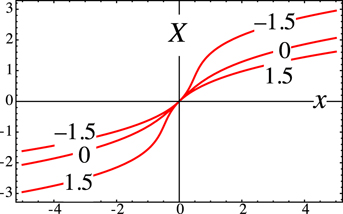
Figure 1. Mappings X(1)(x; 1, G1, 1) (equation (2.8)) for the indicated values of G1.
Download figure:
Standard image High-resolution image
From the forms of f(x), it is not obvious that the original saddle-point expansion is truncated, i.e. In>N = 0. But it is, as will now be demonstrated for N = 1. Expansion of the exponent function f(x) given by (2.8) for G0 = G2 = 1 gives the derivatives
Substitution into table 1 in the
3. Concluding remarks
In the method described here, an asymptotic technique that usually generates a divergent infinite series has been reverse-engineered to find integrals whose expansions terminate. The exponent functions f(x) for which this is achieved are very special. An explicit test that would determine whether a given f(x) is a member of this class would be useful but I have not been able to find one.
The procedure is easily generalised, in two ways. First to consider exponent functions f(x) initially increasing as xM , rather than x2 as in the saddle-point method; second, to consider integrals over the positive real axis rather than the whole real line. This class of integrals, generalising (1.1), is

The natural mapping is now f(x) = XM . The same Jacobian occurs, and when represented by the same polynomial (2.2), with 2N replaced by N, it leads to the same mapping X(x) (equation (2.4)) as before, also with 2N replaced by N, resulting in the exact truncated series, replacing (2.4),

The exponent function for which this truncated series exactly represents (3.1) is (2.6) with the exponent 2 replaced by M.
A technically more difficult generalisation would be to find truncated versions of uniform asymptotic expansions [10, 11], where saddle-points within the integration range coalesce as a parameter (additional to k) varies.
The parameter k in (1.1) need not be real. If it is imaginary, the analysis still applies, and gives truncated series for the method of stationary phase that is fundamental in diffraction theory [12] as the way to connect wave physics with ray optics or classical mechanics.
The exponent functions f(x) in the canonical integrals possess branch points away from the real axis, at the values x mapped by the zeros of G(X). In familiar asymptotics, such singularities contribute to the divergence of the expansion; for example,  in (1.1) generates the Bessel function
  [13], whose large y expansion, generated by
  , diverges. By contrast, the contributions from the branch-points must cancel for the canonical integrals considered here, because their series terminate.
In order to obtain terminated expansions, we have considered cases where the Jacobian G(X) is a polynomial in X. But any function G(X) for which the integral  can be evaluated analytically leads to integrals that can be evaluated exactly. A class of such integrals corresponds to G(X) = 1 + H(X), where H(X) is any odd function. These integrals are not of the form (1.1) because their exponent functions f(x) depend on k.
Acknowledgments
I thank Professor C J Howls and Professor Pragya Shukla for helpful comments. This research started in 1980 while I enjoyed the hospitality of the Gleb Wataghin Institute of Physics at UNICAMP, Brazil.
Appendix.: Saddle-point integration coefficients
With computer algebra, it is not difficult to generate the coefficients In in (1.3), in terms of the derivatives fn . Table 1 shows the first few. The book [8] conveniently lists more: not only the coefficients In for n ⩽ 4, but also their dependence on the derivatives of a k-independent prefactor in the integrand, and the coefficients of half-integer powers of k that occur if the integration in (1.1) is restricted to the positive real axis (as in (3.1) with N = 2).