
Abstract
When two isolated systems are brought into contact, they relax to equilibrium via energy exchange. In another setting, when one of the systems is driven and the other is large, the first system reaches a steady state which is not described by the Gibbs distribution. Here, we derive expressions for the size of energy fluctuations as a function of time in both settings, assuming that the process is composed of many small steps of energy exchange. In both cases, the results depend only on the average energy flows in the system and the density of states, independent of any other microscopic detail. In the steady state, we also derive an expression relating three key properties: the relaxation time of the system, the energy injection rate and the size of the fluctuations. The framework is modular and allows generalizations to other setups, such as a system coupled to two baths at different temperatures.
Export citation and abstract BibTeX RIS
1. Introduction
In this paper, we consider two closely related non-equilibrium problems. In the first problem, two systems which are coupled to each other but isolated otherwise are allowed to exchange energy, see figure 1(a). The systems start with arbitrary initial energies and eventually reach equilibrium. It is natural to ask: how do the initial energies evolve in time as the two systems approach equilibrium? For example, one might imagine measuring the energy of a teacup as it cools, or the equilibration of a mesoscopic system of two atomic gases, initially prepared at two different temperatures. In the second problem we consider, one of the two systems is also driven by an external protocol, see figure 1(b). This is achieved, for example, by applying a time-varying field which repeatedly returns to its initial form. When the second system is much larger than the first, it acts as a dissipative bath, and the first system eventually settles to a non-equilibrium steady state. This scenario serves as a generic model for driven-dissipative systems, which describe a broad range of phenomena [1–3]. Here, one can ask how the first system reaches a steady state, and what are the properties of this non-Gibbsian steady state.

Figure 1. The energy fluctuations in the two set-ups. (a) Exchange of energy between two systems. (b) A system driven by an external force and attached to a bath. (c) A typical evolution of E1(t) (dashed line) fluctuates around the average 〈E1〉(t) (solid line). Equations (3) and (4) relate the size of these fluctuations to the average 〈E1〉(t).
Download figure:
Standard imageAs the dynamics of a system are affected by the detailed microscopic state, repeating the same experiment will lead to different outcomes. Specifically, a measurement of the energy as a function of time will yield different results, see figure 1(c). The variations between experiments might average-out in large, thermodynamic systems, or when the driving protocol applied is quasi-static. However, they can be significant when the drive is not quasi-static and in small or mesoscopic systems, which are of current experimental interest [4–6]. The dependence of these fluctuations on the dynamics makes general statements scarce, and one typically has to resort to the study of specific models.
The setup in figure 1(b) but without interaction with system 2 (so that system 1 is isolated) was recently studied in [7]. It was shown that if the drive induces many small (but still irreversible) changes in the system's energy, then the distribution of energies at a given time depends only on the energy injection rate, and is independent of any other details of the system or drive.
Here, we quantify energy fluctuations in a much broader setting of the two canonical scenarios described above. The scenario of equilibrating systems is modeled by two isolated systems which are allowed to interact. In the scenario of a driven-dissipative system, one of the systems is driven as in [7], and the second is taken to be very large, so as to model a bath. The resulting theory is exact to order 1/N, where N is the number of degrees of freedom of the smaller system, thus being highly relevant to mesoscopic systems, where energy fluctuations may be significant. Conditions on the drive are similar to those in [7]. For the two coupled systems, we require that the energy flow between the two systems is slow, so that each of the two systems separately is close to microcanonical equilibrium at its energy (see below for the exact conditions). In addition, in the driven-dissipative case we assume that the driving and the coupling to the bath are statistically independent processes. The results are insensitive to almost all microscopic details of the systems, depending only on the average energy flows from the drive to the system and between the systems as a function of time, and on the density of states. We stress that the assumptions made do not imply that the combined system (composed of systems 1 and 2) is close to equilibrium, but only that each of the systems separately is close to equilibrium within its energy shell. Our main results are (1) equations (3) and (4), which quantify the variance of the energy fluctuations as the system approaches its steady state (which is equilibrium when no drive is present), (2) equation (5), which relates three main quantities at the steady state: the variance of the energy fluctuations, the average rate of energy flow through the system and the relaxation time of energy fluctuations. In addition, we show that the approach is modular, and may be applied to other settings. As an example, we study a system connected to two external baths. The validity of the results and their use is illustrated in a system of colliding hard spheres and an interacting spin system.
Before turning to a systematic derivation, we first sketch the approach used. To understand the energy exchange behavior, note that the assumptions of weak interaction and slow energy exchange between the systems lead to processes comprised of many small independent energy exchanges. This, much like a particle in water, leads to a diffusive (Langevin) behavior; in our case the diffusion is in the energy plane (see section 3 for a systematic derivation). The state of the combined system is specified by a point in the (E1, E2) plane, and the diffusion takes place in this plane. However, in both scenarios, of equilibrating systems and driven-dissipative systems, one can specify the state by considering E1 alone. For equilibrating systems, this is possible when the initial total energy Etotal = E1 + E2 is fixed, so that E2 can be considered to be a function of E1. In the case of driven-dissipative systems, E2 drops completely from the equations when we take system 2 to be much larger than system 1. This is because system 2 acts as a thermal bath whose properties are insensitive to the changes in E2 (see section 3 for details).
One can therefore consider the probability distribution P(E1) of E1, which will satisfy a Fokker–Planck (FP) (drift-diffusion) equation

where A1(E1), B11(E1) are functions which depend on system details. They do, however, obey the following relation, which is the key to the results which are described below:

where A2 is the average rate of energy exchange between systems 1 and 2, see figure 1(b), AF ≡ A1 + A2 is the rate of energy injected into the system by the drive,  , for i = 1, 2 are the (microcanonical) inverse temperatures of system i at energy Ei and Si(Ei) is the entropy of system i. Note that β1 and β2 are well-defined functions, depending only on the density of states of the system, and unrelated to the driving mechanism and the interaction between the systems. Moreover, β1 can be very different from β2, so the combined system may be arbitrarily far from equilibrium. When system 2 is a bath, A2 is only a function of E1. In the case of equilibrating systems AF = 0, and equation (2) reduces to 2A1 = (β1 − β2)B11. Equation (2) is exact up to corrections of order 1/N, and requires that the energy transfers be slow compared with the relaxation times of each of the systems separately.
We comment that formally slowness enters as a set of conditions on the smallness of higher order cumulant of the work during the relaxation time of the system. For processes which involve an external drive, let ΔEF be the size of the random jump in energy associated with this process. As discussed in the derivation section, we require that β21〈(ΔEF)3〉c ≪ 〈ΔEF〉. Similarly, let ΔEB be the amount of energy exchanged between the systems in a single jump. Then we require (β1 − β2)2〈ΔE3B〉c ≪ 〈ΔEB〉. These conditions can also be used to reason for the validity of the FP equation. By the independence of the steps, the third cumulant of the total energy is expected to grow linearly with the number of steps Nsteps, and therefore its effect on the energy distribution grows as N1/3steps, and is therefore small. For derivations of FP equations along this line of reasoning see, for example, [12]. With equations (1) and (2), we derive all the results described below.
The paper is organized as follows. In section 2, we summarize the main results of this work. In section 3, we derive these results, which follow from equation (2) in the two scenarios of equilibrating and driven-dissipative systems. In section 4, we apply the main results to two example systems.
2. Results
2.1. Approach to the steady state
We start by considering the approach of the combined system (composed of systems 1 and 2) to its steady state. If no driving is present (scenario 1), then this steady state is thermal equilibrium. We derive an expression for the evolution of the variance σ21 = 〈E12〉 − 〈E1〉2 during the entire equilibration process. The result is derived in section 3 by solving for the evolution of the first two moments of equation (1), and using the key relation, equation (2).
We find for the equilibrating systems that the variance is given by

Here, 〈E1〉0 and  are 〈E1〉 and σ21, respectively, at the initial time. Recall that Etotal = E1 + E2 is held constant in this expression. It is easy to extend these results when Etotal varies between experiments. It is interesting to note that when β2 is set to zero, this expression is identical to that obtained for a single-driven isolated system [7]. This means that within this theory, driving a system is formally equivalent to attaching it to a bath with infinite temperature. It is straightforward to show, that when system 2 is a bath, so that β2 can be taken to be a constant, the width σ21 approaches the equilibrium value:
  , where Eeq is the equilibrium value of 〈E1〉 and C is the heat capacity (see e.g., [13]). To see this, note that at equilibrium A1 must vanish, and β1 = β2. Therefore, the entire expression for σ21 is controlled by the final approach of E to Eeq where
  ,
,  and the equilibrium expression follows. Note that away from the final equilibration regime A1(E) need not be linear.
In the case of driven-dissipative systems (when system 2 is large), we obtain for the variance

where Z = [1 − β2AF/(β1A1)]/(β1 − β2). Equations (3) and (4) are our main results for the approach to the steady state. They predict the size of fluctuations in E1 around its average value. They depend only on the rates of energy injection into the system AF (which is zero for equilibrating systems) and the rate of energy transfer to the bath A2. In principle, both these quantities can be measured separately: as a consequence of the independence of the drive and interaction between the systems, AF can be measured by the rate of energy absorption when system 1 is isolated, and A2 in an equilibration experiment without the drive.
2.2. Steady-state fluctuations
The framework described above can also be used to study fluctuations in the steady state of driven-dissipative systems, specifically fluctuations of E1 around 〈E1〉. Typical fluctuations around the steady state are expected to decay exponentially (see section 3),  where e1 ≡ E1 − 〈E1〉. τ is the relaxation time to the steady state. When AF ≠ 0, namely for a driven-dissipative system, we find that

This is our main result for the steady state of driven-dissipative systems. AF is the rate of energy injected into the system from the drive. In the steady state, this energy is then dissipated into the bath. This expression therefore relates three central quantities characterizing the steady state: the size of the energy fluctuations σ21, the rate of energy dissipation AF and τ which is the relaxation time in the steady state.
2.3. Modularity
The above results can be easily generalized to analyzing other settings. For example, consider a setup where a system is attached to two baths, at temperatures β2 and β3, see figure 2. The system approaches a steady state. Here one can show that the size of the variance during the approach is given by equation (4) now with Z(E1) given by

where A2(E1)andA3(E1) are the average energy transfer rates and β1(E1) is the microcanonical temperature of the system at E1. For the steady state, one obtains

where AF is the average rate of energy passing from one bath, through the system, to the other bath. Other more elaborate setups may be constructed similarly.
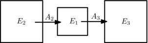
Figure 2. A system attached to two baths.
Download figure:
Standard image3. Derivation
To derive the results presented in section 2, we consider the evolution of the energies in the (E1, E2) plane, where E1andE2 are the energies of systems 1 and 2, respectively. Consider a series of changes in E1andE2, each taking place over a time interval Δt. The changes in E1 and E2 result from the interaction between the systems and from the drive. The drive is implemented by varying a parameter λ in the Hamiltonian which repeatedly returns to some baseline value after a time interval Δt. As in [7] we assume that the energy changes due to the drive in the time interval Δt are small, in a sense specified below. In addition, we assume that τR ≪ Δt, where τR is the relaxation time of each of the isolated systems separately, and without any external drive. Thus, after time Δt many typical relaxation times τR have passed, and the system has forgotten all information about its state except its total energy (which is assumed to be the only conserved quantity), and is hence close to microcanonical equilibrium. The energy changes ΔE1, ΔE2 during non-overlapping time segments of duration Δt are then independent, and depend only on the total energy in that time.
The changes in ΔE1, ΔE2 must obey certain relations. These relations follow, ultimately, from Liouville's equation, or the unitarity of the dynamics in quantum cases. Consider first scenario (b) in figure 1, but with no interaction between systems 1 and 2. The drive consists of many small perturbations to system 1, where the Hamiltonian is varied and repeatedly returns to its original form. In [7] it was shown, that in this case, the change in energy of the system ΔEF when the drive returns to its original state must obey 〈exp ( − β1ΔEF)〉 = 1. Here,  , for i = 1, 2 are the (microcanonical) inverse temperatures of system i at energy Ei, Si(Ei) is the entropy of system i and the angular brackets denote averaging over the initial microscopic states with energy E1. This relation is essentially a Jarzynski relation for isolated systems. Assuming that the changes are small [7] (for a different approach see [10]), we take the logarithm ln 〈exp ( − β1ΔEF)〉 = 0 and expand to second order to find

where N is the number of degrees of freedom. This holds when β21〈(ΔEF)3〉c ≪ 〈ΔEF〉 and  , where
  is the extensive specific heat. The first condition ensures that there are no corrections from the third cumulant in the expansion, the second relation ensures that β1 does not change significantly in one jump and is usually a much weaker condition, and ensures the validity of the Jarzynski relation. These conditions and others cited below are derived in appendix A.
We expand on this result by using a variant of the exchange fluctuation relation [11] which describes the energy flow between two systems. For a weak interaction between the two systems, typically corresponding to slow exchange of energy between them, the entropy of the combined system is additive S(E1, E2) = S1(E1) + S2(E2). In this case 〈exp ( − (β2 − β1)ΔEB)〉 = 1, where β1(E1), β2(E2) are the microcanonical temperatures of the (otherwise isolated) systems, and ΔEB is the amount of energy transferred from system 1 to system 2. Under small work assumptions, we expand ln 〈exp ( − (β2 − β1)ΔEB)〉 = 0 to obtain

This holds when (β1 − β2)2〈ΔE3B〉c ≪ 〈ΔEB〉, and  . This is the key relation which will be used below to describe the evolution of fluctuations in equilibrating systems (scenario (a) in figure 1).
In the scenario of a driven-dissipative system, we combine these two results. We take system 2 to be large, so as to model a bath, and assume further that the driving mechanism and the interaction with the bath produce independent changes in E1, e.g., when the drive and interaction processes act on different modes, on different parts of the systems, etc. Then the two relations (8) and (9) may be combined. The change in E1 is ΔE1 = ΔEF − ΔEB and the change in E2 is given by ΔE2 = ΔEB. We define for i, j = 1, 2,
where Ai is simply the average energy change per unit time in system i. Note that Ai, Bij are functions of (E1, E2).
The assumption of independence of ΔEF, ΔEB gives 〈ΔE21〉 = 〈ΔEF2〉 + 〈ΔE2B〉, which combined with equations (8) and (9) gives equation (2), where AF ≡ A1 + A2 is the rate of energy injected into the system by the drive. As are equations (8) and (9), this result is exact up to corrections of order 1/N, and requires  . In the case of equilibrating systems, AF = 0 and equation (2) reduces to 2A1 = (β1 − β2)B11.
Under conditions of many small independent jumps, and much like when a Brownian particle is displaced by many small kicks, the jumps in the (E1, E2) result in an FP equation. The FP equation is a drift-diffusion for the probability distribution P12(E1, E2), which reads
where Ai, Bij for i, j = 1, 2 are precisely the functions of (E1, E2) described above. Equation (10) is valid under the same above conditions on the third cumulants of ΔE1, ΔE2 [12]. It is then more convenient to work with the marginal probability distribution of E1 alone: P(E1) ≡ ∫dE2P12(E1, E2). As in the different scenarios only E1 is needed, we can integrate equation (10) over E2 to obtain equation (1).
We derive an expression for the evolution of the variance σ21 = 〈E12〉 − 〈E1〉2 during the entire equilibration process. Proceeding similarly to [7], we take the first two moments with respect to E1 of equation (1):

The assumptions on the smallness of ΔEi prescribed above imply that ΔEi can scale at most as O(N); therefore, Ai = 〈ΔEi〉/Δt grows as O(N) at most, and using equation (2), we see that σ21 grows as O(N) at most; hence the distributions are narrow, their widths' scaling subextensively, at most as N1/2. When A scales as N the width scales as in equilibrium. Therefore, up to corrections of order 1/N, 〈A1〉 can be taken to depend on 〈E1〉 alone, and the change of 〈E1〉 in time will be monotonic (since when A changes sign, ∂t〈E1〉 = 0 and the change in 〈E1〉 stops). Combining the two equalities in equation (11) and linearizing A1 within the width of the probability distribution, we find

where Z(〈E1〉) ≡ B11/(2A1). Solving the ordinary differential equation (12) and using equation (2), we find for the equilibrating systems that the variance is given by equation (3).
3.1. Steady-state fluctuations
At the steady state the probability distribution Ps(E1) is independent of time. As ∂t〈E1〉 = 〈A〉 = A(〈E1〉), at the steady state A(〈E1〉) must vanish. Using the narrowness of the distribution (recall that the width scales at most as N1/2), we expand A1 and B11 to lowest order in e1 ≡ E1 − E01:

where Bs and τ are constants. Equivalently, in this regime the FP equation describes the Brownian motion of the energy in a harmonic potential  , where the white noise η(t) satisfies 〈η(t)η(t')〉 = δ(t − t'). τ is then interpreted as the relaxation time, as can be seen from the two time correlation functions
  . The variance of the energy fluctuations is given by σ21 = 〈e1(t1)2〉 = Bsτ/2.
When AF = 0, equations (2) and (13) imply that . Then expanding β1 around β2 as done above, we find that
  which again reproduces the canonical distribution width. The present derivation gives a dynamic interpretation to this formula.
When AF ≠ 0 namely for a driven-dissipative system we find, using A1(E01) = 0 in equation (2), and σ21 = Bsτ/2, we obtain equation (5).
4. Applications
We now present two examples of systems where the above framework applies. The first is a gas of hard spheres, with two different particle types which form the two systems, or the system and the bath, see figure 3(a). The second system is a chain of interacting planar spins (the XY-model), attached to two baths at different temperatures, see figure 3(b).
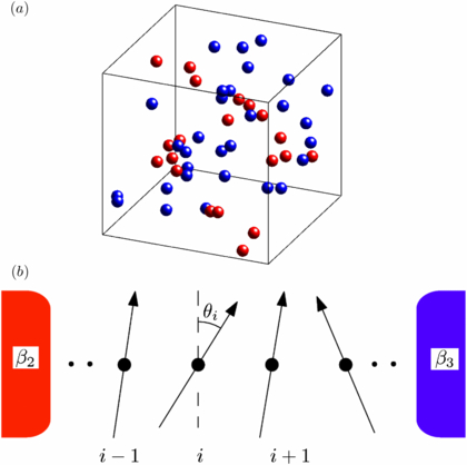
Figure 3. Example systems. (a) A gas of hard sphere, with two particles of two different masses. (b) A spin chain coupled to two baths at different temperatures.
Download figure:
Standard image4.1. Hard sphere system—molecular dynamics simulations
We now illustrate our main results on a gas of hard-sphere particles in a box, simulated by an event-driven molecular dynamics simulation [8]. The simulations demonstrate the validity of the theory for fully deterministic dynamics (apart from bath particles, where a bath is present). In addition, the simulations involve relatively small systems, with just few tens of particles, thus demonstrating the applicability of the predictions to small systems. The systems are completely mixed, making this setup more challenging.
The hard-sphere gas is composed of N1 particles of mass m1 and N2 particles of mass m2, all of equal size, corresponding to systems 1 and 2 respectively, see figure 3(a). Although the entropy of the two systems between collisions indeed factorizes, the collision process involves a strong interaction, which changes the velocities of the particles by a significant amount. A collision calculation shows that if the two masses are very different, then the energy transfer in each collision is small. In this case, energy transfer occurs over many collisions, fulfilling the assumption of timescale separation (see above). In what follows, we take m1 = 10−4, m2 = 1. (Throughout we use arbitrary units.) The large ratio of masses allows us to demonstrate the validity of the results on a single set of system parameters, for a wide range of driving strengths. The results still hold for a smaller mass ratios, albeit in a narrower range of validity. The box is a unit cube with reflecting boundary conditions, and the particles are taken to occupy a volume fraction of 0.05.
We first consider the approach to equilibrium of two systems in contact, figure 1(a), to be compared with the predictions of equation (3). We take N1 = 30 for the first system and N2 = 20 for the second system. N1andN2 are chosen to be relatively small in order to test the theory on a mesoscopic system. The initial velocities are sampled from a Maxwell–Boltzmann distribution with β1 = 60 and β2 = 3, corresponding to average energies per particle of 〈E1〉/N1 = 0.025 and 〈E2〉/N2 = 0.5. We start all runs from a fixed total energy Etotal = 〈E1〉 + 〈E2〉, by performing a (small) rescaling of the m2-particles' velocities. Gathering statistics over many runs, we calculate at each time the average energy 〈E1〉(t) and the variance σ21(t). The function A1(〈E1〉) is obtained by plotting A1(t) = d〈E1〉/dt as a function of 〈E1〉(t). Given A1(〈E1〉)1, we use equation (3) to predict σ21(〈E1〉), and find a good fit with the simulation results, see figures 4(a) and (b).

Figure 4. (a+b) Equilibration of a system of 50 particles with two different masses. In (a), E1(t) in a single run (solid line), and the average energy 〈E1〉(t) (dashed line), used to calculate A1 are shown. In (b) simulation results for 〈E1〉 versus σ21 (dots) are compared to theoretical predictions (solid line), equation (3). (c) Test of equation (5) for a driven-dissipative system.
Download figure:
Standard imageWe now turn to the driven-dissipative scenario and test equation (5) for the steady state. We run simulations on a system with N1 = 10 and N2 = 50 particles. System 1 is driven by applying short impulses to the m1-particles, changing their velocity by Δv = Fδt/m1, where F is a constant force and δt is the impulse duration. This impulse is applied at a constant rate. In order to mimic the behavior of a very large system 2, the velocity of the m2 particles is changed upon reflection from the wall [9], so as to maintain a constant 〈E2〉. The quantities τ, AF, β1 and σ21 are computed from the numerics. The energy of system 2 is maintained at 〈E2〉/N2 = 1/2, or βM = 3. Figure 4(c) shows the results obtained for the two sides of equation (5) as a function of β1/β2 for different strengths of the drive. Good agreement is found over a wide range of drive strengths and temperature differences. In this range, AF increases by a factor of 1000, σ21 by a factor of 17 and the relaxation time τ decreases by a factor of 3.
4.2. XY spin chain
In the second example, we consider a one-dimensional XY model. In this model, a two-dimensional vector is associated with each site. The interaction between neighboring sites i and j is given by Hij = 1 − cos (θi − θj), where θi is the angle of the vector at site i. The total Hamiltonian is H = ∑〈i, j〉Hij, running over all neighboring pairs; in the case of a linear spin chain with N spins, this becomes H = ∑N − 1i = 1cos zi, where zi = θi + 1 − θi.
We attach the system to baths at both ends of the system, with inverse temperatures β2 and β3, and demonstrate the derivation of equation (7) in this case. A bath is modeled by adding an interaction to the leftmost (and similarly for the rightmost) spin θ1, which applies random changes to the angle of that spin. The changes in the angle θ1 are taken in the range −α ⩽ δθ1 ⩽ α, with α ≪ 1, and at rates

where δe(δθ) = −[cos (z1 + δθ) − cos z1] is the change in energy due to the change in θ1 and w0 is a constant setting the overall timescale. This interaction functions as a bath with temperature β2. The last spin, θN, is attached to a bath at temperature β3, by applying a similar protocol with β2 replaced by β3.
We now calculate the first two moments of the energy transfer from the bath to the system. Note that the steady-state energy and fluctuations will be given by the combined effect of the two baths. We now use the assumptions described above, namely that the energy exchanges with the bath are slow compared with the relaxation time of the system. Here this enters by assuming that α ≪ 1 at a fixed w0. As a consequence, the system at a given time is approximately in a microcanonical equilibrium. This means that up to 1/N corrections z1 is distributed with a Boltzmann weight: P(z1)∝exp (β1cos z1), where  is the microcanonical temperature of system 1. The average change in the energy is given by
where In(β) is the modified Bessel of the first kind. The dependence on energy enters through the microcanonical energy–temperature relation:  . A12, B12 satisfy 2A12 = (β1 − β2)B12, which is precisely equation (2) for this system (as AF = 0 for two coupled systems without any drive). Similarly, if the spin θN is attached to a bath at temperature β3, then 2A13 = (β1 − β3)B13. The last two relations are valid more generally, as discussed in previous sections, and encode all the information on the system that is required to derive equations (6) and (7). For example, to obtain equation (7), we attach the system to two baths at temperatures β2, β3 acting independently at both sides of the chain. Then (using the conventions of figure 2), A1 = A12 − A13 and B1 = B12 + B13. At the steady state one has (see section 3) σ21 = B1τ/2, which together with the relations 2A12 = (β1 − β2)B12, and 2A13 = (β1 − β3)B13 gives equation (7).
5. Conclusions
In this paper, we considered several canonical non-equilibrium scenarios, in which energy is transferred between two or more systems, or as work from a drive. We find a specific regime where universal statements on the energy fluctuations during relaxation to the steady state and at the steady state can be made. The results are applicable to systems in various fields. The framework can be extended to other more elaborate settings, such as ones involving a larger number of systems.
Acknowledgments
We are grateful to Luca D'Alessio, Dov Levine, Daniel Podolsky, Anatoli Polkovnikov and Yair Shokef for many useful discussions and comments. The work was supported by a BSF grant. YK thanks G M Schutz.
Appendix
A.1. Derivation of equation (3)
In what follows, we first derive equation (3) of the main text, and then proceed to carefully analyze the conditions for its validity. To derive equation (3) we look at two times t, t + Δt at which the driving protocol has returned to its original state, i.e. where H(t) = H(t + Δt), where H is the Hamiltonian of the combined system. As discussed in section 1 'framework and assumptions', we assume that both subsystems are relaxed in their respective energy shells, with energies E1 and E2, at times t and t + Δt. We denote the changes in E1, E2 during the time interval Δt by ΔE1, ΔE2 respectively, and define ΔEB and ΔEF via

ΔEB is the energy transferred from system 1 to system 2, and ΔEF is the work done on system 1 by the external drive.
Under these conditions, Liouville's theorem or the unitarity of the dynamics, together with micro-reversibility of the dynamics, imply a Crooks relation for the combined isolated system [14–16, 7]2

where  is the probability of a transition (E1, E2) → (E1 + ΔE1, E2 + ΔE2), and
  is defined similarly, only with respect to the reversed protocol, defined by the dynamics generated by the time-reversed Hamiltonian
  . Here, we have used the assumption of the additivity on the entropy, valid for weak interactions, S(E1, E2) = S1(E1) + S2(E2), see the main text.
We approximate  ; this introduces errors which are of order 1/N, as shown below. By the assumption of independence of the driving and interaction mechanisms, ΔEB and ΔEF are statistically independent, and we can write
  . The Crooks relation then reads

Integrating over ΔEF, ΔEB gives a Jarzynski relation

Rearranging the equation, noting that  and integrating gives

Together the two relations yield

Taking the logarithm of these relations and expanding to second order gives relations (1) and (2) of the main text.
A.2. Conditions for validity of equation (3)
We now discuss the conditions for the validity of the above derivation. In it we have made the following approximations. First, we have assumed that  . To find the next correction, we take
  . Following the above derivation, one obtains equation (1) together with the first correction

where 〈ΔE2F〉c = 〈ΔE2F〉 − 〈ΔEF〉2 is the second cumulant of ΔEF. As β1 is an intensive and E1 extensive, the term  introduces corrections of order 1/N which we neglect. Similarly, equation (2) becomes

and the corrections to equation (2) are of order 1/N for the same reason.
The second approximation involves taking Si(Ei + ΔEi) − Si(Ei) ≃ βiΔEi. Again, we incorporate the next correction,  . To this order equations (A.1) and (A.2) read

respectively, which reduce to the above relations if S''1〈ΔEF〉〈ΔEB〉 ≪ 1. Since  (here the Boltzmann constant kB = 1, making
  unitless) this condition reads
Now we can expand  to next order and find

As 〈ΔE2F〉 = 〈ΔEF〉2 + 〈ΔE2F〉c this becomes

The term β21 + S1'' = β21[1 + O(1/N)], since  . Comparing the first and last terms gives the condition
  or
or
In addition, the third cumulant must be small, β31〈ΔEF3〉c ≪ β1〈ΔEF〉 or
A similar argument for  yields the requirement
For β2 − β1 of order β1 and β2, this is satisfied if  for i, j = 1, 2. Close to β1 = β2, both 〈ΔEB〉 and |β2 − β1| go to zero, and this condition may be hard to test. However, 〈ΔE2B〉c remains regular (see discussion in section 2.2 in the main text), and using 2〈ΔEB〉 = (β2 − β1)〈ΔE2B〉c, we obtain an equivalent relation
as  , we obtain the condition
cited in the main text.
Footnotes
- 1
Incidentally, 〈E1〉(t) is found to fit very well to a function of the form E = Efintanh 2(a + bt), or A1∝〈E〉1/2(〈E〉 − Efin), allowing us to write a closed analytical expression for σ21(〈E〉). This can be understood by calculating the rate of energy transfer, taking the collision rate to depend only on the velocity of the lighter, and hence faster, m1 particles.
- 2
In the quantum mechanical setting, we assume that the initial and final density matrices are diagonal, as in [7], and that there is no significant entanglement between the two systems.