
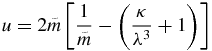
Abstract
The restricted rhomboidal five-body problem (RRFBP) is a problem in which four positive masses, called the primaries, move two by two in circular motions such that their configuration is always a rhombus, the fifth mass being small and not influencing the motion of the four primaries. In our model, we assume that the fifth mass is in the same plane of the primaries and that the masses of the primaries are m1 = m2 = m and  and the radius associated with the circular motion of m1 and m2 is
 ![$\lambda \in [1,\sqrt{3}]$](https://content.cld.iop.org/journals/1751-8121/44/48/485204/revision1/jpa396475ieqn2.gif) and the one for the masses of m3 and m4 is 1. Similar to the circular restricted three-body problem, we obtain the first integral of motion. The Hamiltonian function which governs the motion of the fifth mass is obtained and has two degrees of freedom depending periodically on time. We use a synodical system of coordinates to eliminate the time dependence. With the help of the Hamiltonian structure, we characterize the regions of possible motion. We show the existence of equilibrium solutions along the coordinate axis as well as off them. We verify that the number of equilibria depends on λ and there can be 11, 13 or 15 equilibrium solutions all unstable. We prove the existence of periodic solutions with short as well as long period. Also we prove the existence of transversal ejection–collision orbits (binary collisions) for certain large values of the Jacobi constant, for an uncountable number of invariant punctured tori in the corresponding energy surface.
and the one for the masses of m3 and m4 is 1. Similar to the circular restricted three-body problem, we obtain the first integral of motion. The Hamiltonian function which governs the motion of the fifth mass is obtained and has two degrees of freedom depending periodically on time. We use a synodical system of coordinates to eliminate the time dependence. With the help of the Hamiltonian structure, we characterize the regions of possible motion. We show the existence of equilibrium solutions along the coordinate axis as well as off them. We verify that the number of equilibria depends on λ and there can be 11, 13 or 15 equilibrium solutions all unstable. We prove the existence of periodic solutions with short as well as long period. Also we prove the existence of transversal ejection–collision orbits (binary collisions) for certain large values of the Jacobi constant, for an uncountable number of invariant punctured tori in the corresponding energy surface.
Export citation and abstract BibTeX RIS
1. Introduction
Dynamical systems with few bodies (three) have been extensively studied in the past and various models have been proposed for research aiming to approximate the behavior of real celestial systems. There are many reasons for studying the five-body problem besides the historical ones, since it is known that approximately two-thirds of the stars in our Galaxy exist as part of multi-stellar systems.
We understand that in order to make this problem astronomically more interesting, it would be necessary to discuss the stability of the four-body rhomboidal configuration. In fact, such a study is in progress in a slighter broader sense. In a paper to appear soon, we investigate not only the stability of the four-body rhomboidal configuration under the Newtonian potential, but also under a Manev kind potential. We observe that the instability of such a configuration would not make the problem less interesting in its mathematical approach; only it would mean the improbability of finding a planetary system with four suns in a rhomboidal configuration.
In this work, we study the motion of a body of negligible mass under the Newtonian gravitational attraction of four bodies of masses m1, m2, m3 and m4 (called primaries) moving two by two in circular periodic orbits around their center of mass fixed at the origin of the coordinate system. At any instant of time, the primaries form a rhomboidal configuration of the four-body problem which is a particular solution of the four-body problem. In our model, we will assume that m1 = m2 = m and  and the radius associated with the circular motion of m1 and m2 is a, and the one for the masses m3 and m4 is b. In particular, m1 and m2 are in one of the diagonals of the rhombus and m3 and m4 are in the other diagonal (see figure 1).

Figure 1. The restricted rhomboidal five-body problem.
Download figure:
Standard imageTo study the position of the infinitesimal mass, m5, in the plane of motion of the primaries, we use either the sideral system of coordinates or the synodic system of coordinates (see [3] or [8] for details). In the synodic coordinates, the four point masses m1, m2, m3 and m4 are fixed at (a, 0), ( − a, 0), (0, b) and (0, −b), respectively. In this paper, the restricted rhomboidal five-body problem (RRFBP) consists of describing the motion of the infinitesimal body, m5, under the gravitational attraction of the four primaries m1, m2, m3 and m4.
In the RRFBP, the equations of motion of m5 in synodical coordinates (ξ, η) with angular velocity ω are
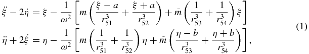
where  ,
,  ,
,  and
and  .
.
Our paper is organized as follows: section 2 is devoted to characterizing the rhomboidal central configuration according to the parameters m,  , a, b and ω. In fact, appropriate relations among them must be satisfied in order to obtain a rhomboidal central configuration and the five parameters will be reduced to only one: λ = a/b. In section 3, we deduce the equations of motion that describe our restricted five-body problem. Section 4 is devoted to proving the existence of the first integral of motion, to present the Hamiltonian formulation and the Hill regions. In section 5, we study the existence of equilibrium solutions as a function of the parameter λ. In section 6, we study the stability of such equilibrium solutions. In section 7, we prove the existence of periodic solutions. In section 8, we prove the existence of transversal ejection–collision orbits (binary collisions) for certain large values of the Jacobi constant, for an uncountable number of invariant punctured tori in the corresponding energy surface and the existence of periodic orbits of long periods.
2. Characterization of the rhomboidal configuration
We consider four bodies with masses m1 = m2 = m and  in a rhomboidal configuration with diagonals 2a and 2b. We will suppose that the four bodies are, two by two, in circular orbits with angular velocity ω and radii a for m1, m2 and b for m3, m4. As is a classical approach in such cases, the system will be treated in a synodical system of coordinates in order to eliminate the time dependence. In such a case, the whole system rotates with constant angular velocity ω, the centripetal forces compensate for the Newtonian attraction and the four bodies are in equilibrium in such a rotating system. For obvious reasons, such a case is called a relative equilibrium. The angular velocity can be picked at will, but, due to Keppler's third law, this would imply restrictions on the other parameters. In the next section, we explain the reason for our choice of ω and why this does not mean any loss of generality to the problem.
If we denote by rj the position of the body with mass mj, then

We consider G = 1 and then the equations of motions of the 4-body problem are given by

in particular, for i = 1, we have

but  , so the above equation reads

and equating the components features

the equation of motion for m2 features the same equation as above and from the equation of motion for m3 (or m4), it results in a similar way that

We note that the problem initially has five parameters related by equations (3) and (4). They both must be satisfied in order to provide us with a central configuration for the rhombus (see [2] for some characterizations of rhomboidal central configuration). They will help us to lower the number of parameters. Physically, the role of ω, the angular velocity, is to compensate for the centripetal force to establish the relative equilibrium, so we will choose a specific value for ω in order to simplify our computations. Most authors choose ω = 1 but we would rather make another choice. Also choosing our mass (or geometric) parameters at will would impose restrictions upon the geometric (or mass) parameters. The choice we make is to simplify the approach to the problem without losing generality.
From equations (3) and (4), we have

and setting λ as the ratio of the semi-diagonals and κ the ratio of the masses, i.e.

relation (5) can be rewritten as

Now we prove the following preliminary result.
Lemma 1. κ = κ(λ) given implicitly by (7) is a continuous, positive, strictly decreasing function in the interval ![$(1/\sqrt{3},\sqrt{3}]$](https://content.cld.iop.org/journals/1751-8121/44/48/485204/revision1/jpa396475ieqn11.gif) ,
,  and
and  .
.
Proof. From relation (7), we easily find that for each λ, there exists only one κ given by

It is easy to check the continuity and the values for  and
and  directly from expression (8), so we only need to prove that such a function is decreasing and then, as a consequence, it will always be positive.
From (8), we obtain

The only term that could make this derivative negative is [(1 + λ2)5/2 − 8(1 + λ5)], so now we look at the function

and we show that its maximum value is below 8, which suffices to tell us that the previous expression is negative and so it is the derivative of κ. Let us see
which is negative for λ ⩽ 1 and positive for λ ⩾ 1, so φ is a convex continuous function; therefore, it reaches its maximum at one of the extremes,  and
and  . Therefore, the lemma is proved (see the graph of κ(λ) in figure 2). Now we can prove the following.

Figure 2. The function κ(λ).
Download figure:
Standard imageProposition 1. The five parameters, ω, m,  , a and b, of the rhomboidal central configuration defined by (3) and (4) can be reduced to only one:
  . More precisely, we can assume, without any loss of generality, that b = ω = 1.
Proof. Rewriting equations (3) and (4) as


we observe that there is no restriction on considering ω = b = 1 for if it were not so, due to the freedom we have for picking the angular velocity ω, for any given b we could just choose  , and considering
  , equations (9) and (10) are clearly equivalent to


which are exactly the equations for the problem with ω = 1 and b = 1. So it is clear that we can treat this as the general case without any loss of generality, since both systems of algebraic equations are equivalent as well as the system formed by the equations of motions. On the other hand, from (11) and (12), it is possible to obtain the useful relations


See the graphs of m(λ) and  in figure 3.
We have somehow inverted the process of finding the central configuration. By the above construction, we have allowed ourselves the freedom to, supposing that b = 1, choose any value for the horizontal semi-diagonal a = λ in the interval ![$(1/\sqrt{3},\sqrt{3}]$](https://content.cld.iop.org/journals/1751-8121/44/48/485204/revision1/jpa396475ieqn25.gif) ; then m and
; then m and  can be determined by relations (13) and (14) and this choice will always feature a central configuration for the problem.
So the only parameter that really matters is the mass ratio λ which can be considered as the horizontal semi-diagonal itself by taking b as the unit of length.

Figure 3. Left: the graph of m(λ). Right: the graph of  , for
, for ![$\lambda \in [1,\sqrt{3}]$](https://content.cld.iop.org/journals/1751-8121/44/48/485204/revision1/jpa396475ieqn24.gif) .
.
Download figure:
Standard imageAs we have observed, the true range of values for λ is the half-closed interval ![$(1/\sqrt{3},\sqrt{3}]$](https://content.cld.iop.org/journals/1751-8121/44/48/485204/revision1/jpa396475ieqn27.gif) , but if we apply the symmetry
, but if we apply the symmetry  then we obtain
  ,
,  , where
  and
and  ; such an observation can also be easily confirmed from (8) from which we easily see that κ(λ−1) = (κ(λ))−1. Thus, we see that treating only the case
  gives us the same information as in
 ![$(1/\sqrt{3},1]$](https://content.cld.iop.org/journals/1751-8121/44/48/485204/revision1/jpa396475ieqn34.gif) . Such behavior is pretty well expected since the change caused by S just corresponds to a rotation of an angle of
. Such behavior is pretty well expected since the change caused by S just corresponds to a rotation of an angle of  in our configuration, and c.c.'s are invariant by rotation. So from now on, unless strictly mentioned, we shall restrict our study to the case
 ![$\lambda \in [1,\sqrt{3}]$](https://content.cld.iop.org/journals/1751-8121/44/48/485204/revision1/jpa396475ieqn36.gif) . The case λ = 1 corresponds to the square configuration. Furthermore, we can include the case
. The case λ = 1 corresponds to the square configuration. Furthermore, we can include the case  , i.e. the limit case when
  . In this case, we clearly have κ → 0 and
  which is the corresponding angular velocity for the relative equilibrium solution for the three-body problem. Also, in this case m → 0, and so such a result makes complete sense. As we expect, in this case our two primaries with positive masses and either one of the other massless primary bodies take the equilateral triangular Lagrangian relative equilibrium positions. Thus, the limit case ends up to be the relative equilateral triangular configuration.
We also remark that our decision to reduce the number of parameters does have a little geometrical cost: taking ω2 = b3 implies that the rhombus cannot have an arbitrary shape because the range of values for λ implies restrictions to its shape; we show this in figure 4. This does not destroy the generality of the problem; it only imposes some restrictions on the geometric shapes of the rhombus we consider here. It is a small price we have decided to pay for the simplicity of the approach. If different rhombus shapes were needed to be studied, the preceding arguments could be rearranged to suit them. We also point out that a change in the ratio of the diagonals cannot take place unless it is compensated by a change in the mass relation, since κ is a function of λ.
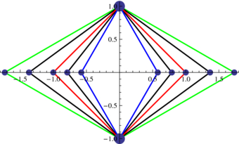
Figure 4. Some possible shapes for the rhombus depending on ![$\lambda \in (1/\sqrt{3}, \sqrt{3}]$](https://content.cld.iop.org/journals/1751-8121/44/48/485204/revision1/jpa396475ieqn40.gif) .
.
Download figure:
Standard imageNow, we present some particular cases as simple examples.
- The square. If λ = 1, we have κ = 1 and by equations (13) and (14),
 .
. - A true rhombus. If κ = 1/2, then by equation (8), λ = 1.378 961 532, and by equations (13) and (14), and m = 1.105 39.
- Rhombus with zero masses. If , then κ = m = 0, and the rhombus has zero masses on the horizontal axis. As we have already observed, this case can be clearly identified with a restricted three-body problem in its Lagrangian relative equilibrium solution, though in this case it should be called something like the 'bi-restricted four-body problem' since it carries both Lagrangian equilibrium solutions at once. An analog case would occur if we allow , for then κ → ∞ meaning that and then we have the same configuration as before rotated by π/2 degrees. In this case, we have m ≈ 0.7698. Again we have a 'bi-restricted four-body problem' but now with the positive masses on the ξ-axis, at the positions and , respectively.


3. Statement of the problem
We consider the problem of studying the dynamics of an infinitesimal body on the plane, moving according to the gravitation field created by the attraction of four bodies moving in a planar rhomboidal configuration according to the previous section. We call this problem the rhomboidal restricted five-body problem (RRFBP). The equation of motion of the body m5 is

where  . Let the orthogonal reference system be

in which we take ω = 1 according to the observation we have made in the previous section. Let r5 = ξe1 + ηe2; then the equations of motion are
where the mutual distances are defined by

4. Preliminary results
Considering the following function, called the effective potential:

we define analogously to the circular restricted three-body problem (see [7]) the function

Proposition 2. C is the first integral of motion of the system (16).
Proof. The derivative of C in relation to time t is

due to (16). Therefore, C is constant along the solutions of the RRFBP.
4.1. Hamiltonian formulation
As is classical in celestial mechanics problems, the Hamiltonian approach is very useful and, therefore, preferable over other approaches.
For synodical systems of coordinates, we follow the well-known procedure described in [8] in order to put problem (16) into its Hamiltonian formulation. We define new variables

with this notation, the RRFBP described by the system (16) assumes a Hamiltonian form, whose Hamiltonian function is

where

In particular, the equations of the RRFBP have the Hamiltonian form

It is clear that the RRFBP has two degrees of freedom, and it is well defined on

which corresponds to  minus four points. These four points are exactly the binary collisions between the infinitesimal body and each of the primaries.
According to the equations of motion, the RRFBP presents an interesting symmetric case. It corresponds to the case where  , i.e. the rhombus is a square.
Finally, we observe that the equations of motion (22) are invariant by the symmetry

that is, if ψ(τ) = (ξ(τ), η(τ), pξ(τ), pη(τ)) is a solution of the system (22), then also φ(t) = (ξ( − τ), −η( − τ), −pξ( − τ), pη( − τ)) is a solution. We note that this symmetry corresponds to a symmetry with respect to the ξ-axis.
4.2. The Hill region
From the definition of the first integral of the RRFBP, we observe that

Thus, the region

is the region of permitted motion, i.e. it corresponds to the so-called Hill region. The curve that is the boundary between the allowed and the prohibited regions of motion is called the zero-velocity curve, and it will be denoted by  . A good comprehension of such sets will provide us with a rich understanding of the nature of the possible motions for the problem.
The Hill region depends on the parameter λ; we represent the function Ω emphasizing such a dependence,

in which we have r251(λ) = (ξ − λ)2 + η2 and r252(λ) = (ξ + λ)2 + η2. Ω(ξ, η, λ) is positive, so the permitted values of C are such that C < 0. Next, we give a list of all possible situations that may appear when this condition is fulfilled.
- (1)ξ → ∞ or − ∞ (respectively, η → ∞ or − ∞) on the, when C → −∞.
- (2)For |C| very large, this implies that (ξ, η) can be sufficiently close to one of the primaries.
- (3)Since ξ2 + η2 is a term in Ω on, small values for −C are not allowed.


In figures 5 and 6, we show the function Ω for three values of λ and in figures 7 and 8, the zero-velocity curves for the same values of λ.

Figure 5. The effective potential Ω. Left: λ = 1; right: λ = 1.3789.
Download figure:
Standard image
Figure 6. The effective potential Ω. Left: λ = 1.65; right: 
Download figure:
Standard image
Figure 7. The zero-velocity curves. Left: λ = 1; right: λ = 1.3789.
Download figure:
Standard image
Figure 8. The zero-velocity curves. Left: λ = 1.65; right:  .
.
Download figure:
Standard image5. Equilibrium solutions
5.1. Equilibria on the coordinate axis
In this section, we study the existence and number of equilibrium solutions in the RRFBP. The equilibrium solutions of the system (16) correspond to the constant solutions of such a system; that is to say the points (ξ*, η*) such that Ωξ(ξ*, η*) = 0 and Ωη(ξ*, η*) = 0 because the right-hand side of (16) is exactly Ωξ and Ωη, i.e.

A simple computation shows that (0, 0) is an equilibrium solution for any values of m and  . In the symmetric case, i.e. λ = 1 (
 ), in [1] it has been proved that any equilibrium solution must be along the diagonal or the mediatrix of the square defined by the primaries.
Since the potential Ω is invariant under the symmetry, (ξ, −η),( − ξ, η) and ( − ξ, −η), we will restrict our computation to the first quadrant: ξ ⩾ 0 and η ⩾ 0. Initially, we look for equilibria along the diagonals of the rhombus. First, we treat the case of the ξ-axis, i.e. η = 0. Then, the equilibria are the solutions of the equation F = 0, where

Let us now simplify the above function by considering  , that is,

In order to study the existence and number of equilibrium solutions along the ξ-axis, we must study separately the cases 0 < ξ < λ and ξ > λ.
Theorem 1. Along the ξ-axis in the RRFBP, there is a unique equilibrium solution satisfying ξ > λ, i.e. out of the rhomboidal configuration.
Proof. For ξ > λ, the function f in (28) assumes the form

Thus, the derivative of the function f is given by
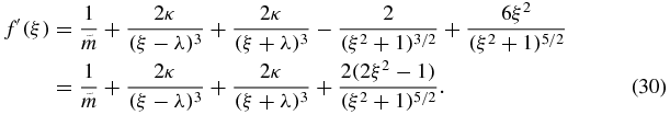
As ξ > λ ⩾ 1, it follows that 2ξ2 − 1 > 0; therefore, f'(ξ) > 0 in this interval. Thus, if ξ > λ, we have that f is an increasing function. On the other hand, since f(ξ) → −∞ if ξ → λ+ and f(ξ) → +∞ if ξ → +∞, we conclude the proof.
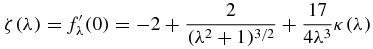
Now we look to what happens when  . Rewriting f, we obtain

From (11), we have  and substituting it into (28), we also obtain that the function f can be represented by

Here we have denoted f by fλ in order to emphasize its dependence on the parameter λ. Then it follows straight from expression (8) that

both of the above expressions will be very useful, so we should use the more convenient one at each time.
The zeros of the above function show us the equilibria of our system on the ξ-axis. The values of the mass ratio parameter λ vary in ![$[1,\sqrt{3}]$](https://content.cld.iop.org/journals/1751-8121/44/48/485204/revision1/jpa396475ieqn62.gif) and the number of equilibria depends on such values as we show below. The function is odd; then ξ = 0 is always a zero of it and another single zero of it has just been shown to exist in the interval ξ > λ. We now restrict our study to ξ ∈ (0, λ) with
and the number of equilibria depends on such values as we show below. The function is odd; then ξ = 0 is always a zero of it and another single zero of it has just been shown to exist in the interval ξ > λ. We now restrict our study to ξ ∈ (0, λ) with  .
.
Lemma 2. There exists  > 0 and a unique
  such that for all λ ∈ (1, λb), fλ(ξ) > 0 for |ξ| < . For all
  , fλ(ξ) < 0 for |ξ| < . That is to say that fλ(ξ) is positive or negative near the origin, depending on whether the value of λ is smaller or greater than λb.
Proof. The expression for f'λ(ξ) is obtained from equation (32) and it is given by

so we have
from which we obtain

From the expression for ζ(λ), it is easy to verify its continuity in ![$[1,\sqrt{3}]$](https://content.cld.iop.org/journals/1751-8121/44/48/485204/revision1/jpa396475ieqn66.gif) and then from (35) and the mean value theorem, it follows that there exists λb such that
and then from (35) and the mean value theorem, it follows that there exists λb such that  . Now we note that

which by virtue of lemma 1 is obviously negative since all its terms are. The uniqueness of λb follows from the fact that ζ(λ) is strictly decreasing. So fλ(0) is increasing for λ ∈ (1, λb) and decreasing for ![$\lambda \in (\lambda _b,\sqrt{3}]$](https://content.cld.iop.org/journals/1751-8121/44/48/485204/revision1/jpa396475ieqn68.gif) near the origin. We also have that fλ(0) = 0 for
near the origin. We also have that fλ(0) = 0 for ![$\lambda \in [1,\sqrt{3}]$](https://content.cld.iop.org/journals/1751-8121/44/48/485204/revision1/jpa396475ieqn69.gif) , and then the result follows.
, and then the result follows.
Remark 1. With the help of the Mathematica, we found λb ≈ 1.239 32 and the graphic of ζ(λ) is given in figure 9 (left). For several values of λ, figure 9 (right) shows the graphs of fλ(ξ), near the origin.

Figure 9. Left: the function ζ(λ). Right: fλ(ξ) for several values of λ and ξ ≈ 0.
Download figure:
Standard imageLemma 3. For all values of ![$\lambda \in [1,\sqrt{\frac{3}{2}}]$](https://content.cld.iop.org/journals/1751-8121/44/48/485204/revision1/jpa396475ieqn70.gif) , we have that fλ(ξ) > 0 for all values of ξ ∈ [0, λ).
, we have that fλ(ξ) > 0 for all values of ξ ∈ [0, λ).
Proof. From equation (34), we obtain

which is clearly positive if  . If
. If  , then f''λ(ξ) > 0 for all ξ so fλ(ξ) is a convex function. Note that
  and this assures us that
  , so that f'λ(0) > 0. Therefore, fλ is an increasing function near the origin but it is also a convex function in the whole interval, so it follows that it is always positive.
Lemma 4. For all values of λ in the interval ![$[1,\sqrt{3}]$](https://content.cld.iop.org/journals/1751-8121/44/48/485204/revision1/jpa396475ieqn75.gif) , we have that fλ(ξ) is an increasing function for
, we have that fλ(ξ) is an increasing function for  .
.
Proof. It follows from expression (34) that for all  , we have that f'λ(ξ) > 0 for all possible values of λ. Thus, the result follows.
Lemma 5. There exists a value λc in the interval ![$(\lambda _b,\sqrt{3}]$](https://content.cld.iop.org/journals/1751-8121/44/48/485204/revision1/jpa396475ieqn78.gif) such that for all values of λ in the interval [1, λc], we have that fλ(ξ) > 0 for all values of ξ such that
such that for all values of λ in the interval [1, λc], we have that fλ(ξ) > 0 for all values of ξ such that  .
.
Proof. The result follows directly from the previous lemma if we show that there exists a value λc for which  if λ ∈ [1, λc]. The existence of such λc is clear from the graphic analysis of the function
  given below. Such λc cannot be smaller than λb for
  for all values of
  and that cannot happen for
  near the origin, at least.
With the help of Mathematica, we have found λc = 1.49; see the graphic of  in figure 10.

Figure 10.  as a function of λ.
Download figure:
Standard imageTheorem 2. For all λ ∈ [1, λb], fλ(ξ) has no zeros for ξ ∈ (0, λ). For all ![$\lambda \in (\lambda _b,\sqrt{3}]$](https://content.cld.iop.org/journals/1751-8121/44/48/485204/revision1/jpa396475ieqn87.gif) , fλ(ξ) has exactly one zero for ξ ∈ (0, λ). In particular, there is, at most, a unique non-zero equilibrium solution of the RRFBP on the ξ-axis, in the interior of the rhombus.
, fλ(ξ) has exactly one zero for ξ ∈ (0, λ). In particular, there is, at most, a unique non-zero equilibrium solution of the RRFBP on the ξ-axis, in the interior of the rhombus.
Proof. The demonstration follows observing the following steps.
- (1)
- (2)If λ ∈ [λb, λc], we know that such functions have only one zero in the interval ξ ∈ (0, λ) and since they are non-negative at ξ = λc, the result follows again from lemma 5.
- (3)If, then we know that their values are negative at ξ = λc, but fλ(ξ) is strictly increasing for and positive when ξ approaches λ, so it must cross the ξ-axis only once.
![$\xi \in [0,\sqrt{3/2}]$](https://content.cld.iop.org/journals/1751-8121/44/48/485204/revision1/jpa396475ieqn88.gif)


![$\lambda \in [\lambda _c,\sqrt{3}]$](https://content.cld.iop.org/journals/1751-8121/44/48/485204/revision1/jpa396475ieqn91.gif)

5.2. Prohibited region for equilibria
In this section, we understand how the equilibria tend to move away from the more massive primaries and closer to the less massive ones. The line that passes through the center of mass between m1 and m3 is given by  . We consider the two mediatrix lines between m1 and m3, and between m2 and m4, respectively, given by R13:
  and R24:
 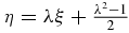 . Let us consider the function f(ξ, η, λ) = Δ1(ξ, η, λ) − Δ2(ξ, η). Clearly f is positive for all values of λ and for the values of (ξ, η) to the right-hand side of R13, and f is negative for values of (ξ, η) to the left-hand side of R24, so, by the continuity of the functions involved, the zeros of f shall be in the region between R13 and R24. We shall denote by Δ0(ξ, λ) the curve of such zeros. The graph of Δ0(ξ, λ) is given in figure 11, for λ = 1.7.

Figure 11. The graph of Δ0(ξ, 1.7).
Download figure:
Standard imageWe consider A and B the regions above and below the line  . Note that when λ = 1, the curves Δ0(ξ, λ) and
  coincide. When λ grows, they separate, and four of such curves and the region between them are shown in figure 12. So, as before, if (ξ, η) is an equilibrium, then Ωξ = 0 and
  .
First suppose that (ξ, η) is to the left-hand side of Δ0(ξ, λ). Then Δ1 > Δ2 and we have
.
First suppose that (ξ, η) is to the left-hand side of Δ0(ξ, λ). Then Δ1 > Δ2 and we have

therefore, we cannot have  , so that region A,
  , is prohibited for equilibria. So there cannot be equilibria in the region above the line which passes through the center of mass and below the Δ0 curve whenever the last one is above the first. On the other hand, the same reasoning prohibited the region above the curve Δ0 and below the line which passes through the center-of-mass curve whenever the last one is above the first (see figure 12).

Figure 12. The region of exclusion: left λ = 1.194 43; right λ = 1.3575.
Download figure:
Standard imageFor the following analysis, let us rewrite the expression for Ωξ and Ωη as follows:

where


According to the previous observation, we can restrict our search to the first quadrant so that in this case, clearly we have Δ1 > 0 and Δ2 > 0, so by (37) in order to have an equilibrium, we must have Δ < 0.
For future use, we need to show that the equilibria cannot be arbitrarily far from the primaries.
Lemma 6. Considering ![$\lambda \in [1,\sqrt{3}]$](https://content.cld.iop.org/journals/1751-8121/44/48/485204/revision1/jpa396475ieqn101.gif) , there are no equilibria in the region ξ ⩾ 0 and η ⩾ 0 whose distance from
, there are no equilibria in the region ξ ⩾ 0 and η ⩾ 0 whose distance from  is greater than or equal to
 ![$\tilde{\rho }(\lambda )=\sqrt[3]{{4\tilde{m}(\lambda )}}$](https://content.cld.iop.org/journals/1751-8121/44/48/485204/revision1/jpa396475ieqn103.gif) and whose distance from m1 = m is greater than or equal to
and whose distance from m1 = m is greater than or equal to ![$\rho (\lambda )=\sqrt[3]{{4m(\lambda )}}$](https://content.cld.iop.org/journals/1751-8121/44/48/485204/revision1/jpa396475ieqn104.gif) .
.
Proof. If  , then
  and therefore
  . But r53 < r54, and so we also obtain
  . Now,
 ![$r_{51}\ge \rho (\lambda )=\sqrt[3]{4m(\lambda )}$](https://content.cld.iop.org/journals/1751-8121/44/48/485204/revision1/jpa396475ieqn109.gif) and in a similar way we obtain
and in a similar way we obtain  , leading to Δ ⩾ 0, which just cannot happen.
Note that the region of exclusion consists of the outside of two circles whose radii depend on the value of λ alone. As the values of λ increase, the circle Cη, centered on the η-axis, grows in size while remaining at a fixed center; meanwhile, the other circle Cξ shrinks and has its center shifted to the right-hand side. Also it is easy to observe that ρ(λ) is never big enough so that Cξ contains Cη. On the other hand, it is not difficult to prove that (λ, 0) is always inside Cη. Also  . As an illustration, we show in figure 13 such regions for three particular cases.

Figure 13. Regions of possible equilibria. Left: the square: λ = 1; center: λ = 1.378 96; right: near the limit case  .
.
Download figure:
Standard imageProposition 3. Let (ξi(λ), 0) and (ξe(λ), 0) be the equilibria located on the ξ axis in the internal or external rhombus configuration, respectively; then ξi(λ) (which exists only for λ > λb) is an increasing function converging to  when
when  and ξe(λ) is a concave function converging to
  when
when  . Thus, all the equilibria on the ξ-axis converge to
  .
.
Proof. It is not difficult to show the monotonicity of ξi(λ) and of ξe(λ) (see figure 14, the zeros of such a function are exactly ξj(λ))), and the monotonicity of ξe(λ) for λ big enough. Since both are limited by  , they both converge to their
  or
or  respectively. Suppose that such limits are
  , where j ∈ {i, e}; then from the definition of an equilibrium and for all allowed values of λ, we must have

where j ∈ {i, e}; since  , Δ1 is limited and the second term goes to 0 because m(λ) → 0 when
  . When we take the limit
  we obtain

but 0 ≠ ξ*j, because of the monotonicity, and we obtain

but r53(ξ*j, 0) = r54(ξ*j, 0) so that we must have r53(ξ*j, 0) = r54(ξ*j, 0) = 2, which can only happen if  which is a contradiction.

Figure 14. fλ(ξ) for various λ and ξ ∈ (0, λ).
Download figure:
Standard imageIn figure 15, we present the graph of the internal horizontal equilibria as a function of ![$\lambda \in [1,\sqrt{3}]$](https://content.cld.iop.org/journals/1751-8121/44/48/485204/revision1/jpa396475ieqn126.gif) , obtained numerically.
, obtained numerically.

Figure 15. The internal horizontal equilibria as a function of  .
.
Download figure:
Standard imageNow we search for equilibria on the η axis, that is, when ξ = 0. The equilibria are then the solutions of the equation G = 0, where

Let us now simplify the above function by considering  , that is,

If 0 < η < 1, then we have that 0 < y < 1/λ, and if η > 1, we must have that y > 1/λ. In order to study the existence of equilibrium points along the η-axis, we will study separately the cases 0 < y < 1/λ and y > 1/λ.
Theorem 3. Along the η-axis in RRFBP, there exists a unique equilibrium satisfying η > 1, (i.e. out of the rhomboidal configuration) and there is no equilibrium inside the rhombus at the η-axis, except for the origin.
Proof. For y > 1/λ, the function g in (39) assumes the form

and its derivative is given by

We use (11) and obtain

and κ = κ(λ) ⩽ 1 so that

Thus, if y > 1/λ, it follows that g'(y) > 0 in this interval; therefore, g is an increasing function. On the other hand, since g(y) → −∞ if y → (1/λ)+ and g(y) → +∞ if y → +∞, we conclude the proof of the first part.
In order to prove the second statement, we note that for 0 < y < 1/λ, the function g in (39) assumes the form

Thus, the derivative of the function  is given by

In the interval under study, it is verified that

because of relations (8) and (14), and  . Thus,
  is increasing and since
  the proof of the second statement follows.
Similar to what happens in the ξ-axis, we have
Proposition 4. Let (0, η(λ)) be the equilibria located on the η-axis, with η > 1; then η(λ) is an increasing function converging to  when
when  .
.
Proof. It suffices to see that the function g is a decreasing function of λ so that its zeros in η grow together with λ; then we have that they must converge, since they are inside a compact set, and they converge to their sup which is the zero obtained when  , that is, 2.39681. The graph of
  is given in figure 16 and the graphic of the vertical equilibria (0, η) as a function of λ is given in figure 17.

Figure 16. The graph of 
Download figure:
Standard image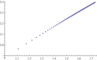
Figure 17. The graph of the vertical equilibria (0, η*) as a function of ![$\lambda \in [1,\sqrt{3}]$](https://content.cld.iop.org/journals/1751-8121/44/48/485204/revision1/jpa396475ieqn138.gif) .
.
Download figure:
Standard image5.3. Equilibria out of the coordinate axis
In this section, we present a few analytical results and some numerical ones in order to provide a general view of the behavior of the bifurcation phenomena which occur as λ increases toward  . For instance, we do not prove the existence of equilibria off the axis and far from the square configuration but we provide numerical evidences to support their existence and find how many they are according to the value of λ. See the graphics in figure 18. They show the level curves Ωξ = 0 and Ωη = 0, for three values of λ the intersections of which are the searched equilibria. We conclude this section with a summary of the number of equilibria as well as a description of how they evolve.

Figure 18. Ωξ = 0 and Ωη = 0. Left: the square: λ = 1; center: a true rhombus: λ = 1.378 96; right: the limit case  .
.
Download figure:
Standard imageWe first analyze what happens near the square case, i.e. when λ = 1. We observe that this configuration presents two equilibria along the mediatrix: one inside the square at (0.493 122, 0.493 122) and a second one at (1.133 07, 1.133 07). Let us consider the following function:

We look at the Jacobian matrix of the above function,

in which we have

We call ϒ(ξ, η, a) the determinant of the above matrix and with the help of Mathematica, we find ϒ(0.493, 0.493, 1) = −52.382 and ϒ(1.133, 1.133, 1) = 2.707 and making use of the implicit function theorem, we obtain that there must exist a neighborhood of λ = 1 such that ξ = ξ(λ), η = η(λ) and F(ξ, η, λ) = F(ξ(λ), η(λ), λ) = 0, for each λ in (1 − , 1 + ) so that (ξ(λ), η(λ)) are equilibria for each value of λ close enough to 1. So we have proved the following result.
Proposition 5. For every λ near 1, there exists a non-zero equilibrium in the form (ξ(λ), η(λ)), in the RRFBP.
Using implicit differentiation and Mathematica, we obtain


which is in accordance with the behavior of the curves of equilibria close to the square configuration (see figure 19).

Figure 19. Behavior of the curves of equilibria near λ = 1. Left: interior equilibria; right: external equilibria.
Download figure:
Standard imageSimilar to what we obtain for the equilibria on the axis, we have the following result.
Proposition 6. Let (ξi(λ), ηi(λ)) and (ξe(λ), ηe(λ)) be the equilibria located in the first quadrant, off the axis in the internal or external rhombus configuration, respectively; then there exist sub-sequences of ξj and ηj still denoted in the same way (ξj(λ), ηj(λ)), for j ∈ {i, e}, that converge to  when
when  .
.
Proof. Clearly from lemma 6, we have that ξj(λ) and ηj(λ) are limited and therefore both must have convergent sub-sequences. We keep the same notation as the original sequences. Let us denote by ξ*j and η*j their respective limits. Suppose first that the limit for the first coordinate is  ; then from the definition of an equilibrium, we must have, for all values of λ,

where j ∈ {i, e}, since  we have that the first term goes to 0 when
  because
  and
and  whatever the value of η*j is; therefore, we must have

and then we obtain

So we must have r53(ξ*j, η*j) = r54(ξ*j, ηj*); therefore, η*j = 0. Again from the definition of an equilibrium, we must have, for all allowed values of λ,

since  ; as before, we take the limit
  and we obtain

but 0 ≠ ξ*j and so  , but as r53(ξ*j, 0) = r54(ξ*j, 0), we have

which is a contradiction, proving the statement for the first coordinates. So  . Now, suppose that η*j > 0; then
  and we obtain

which cannot happen with η*j ≠ 0. This completes the proof.
Figure 20 shows the behavior of both equilibria which are not on the axis, as λ goes to  .
.

Figure 20. The equilibrium curve as a function of ![$\lambda \in [1,\sqrt{3}]$](https://content.cld.iop.org/journals/1751-8121/44/48/485204/revision1/jpa396475ieqn154.gif) . Left: internal equilibria; right: external equilibria.
. Left: internal equilibria; right: external equilibria.
Download figure:
Standard imageWe summarize our results. For all values of λ, there are always four equilibria that never disappear: the origin, of course, and three others external to the rhomboidal configuration, two of which are on the ξ and η axes, respectively. For the internal equilibria, we have that from the square configuration and up to λ = λb = 1.23932, there exist only the internal ones off the axis equilibrium; for λ ∈ (λb, λ* = 1.61027), there exist two internal equilibria one on and one off the ξ-axis. For λ > λ*, these two equilibria become only one which runs on the ξ-axis converging to  (observe figure 20, left). Furthermore, this is also the behavior of the external equilibria on the ξ-axis, so that when
  , they all become a single one, exactly the one corresponding to the Lagrange equilibrium solution.
Proposition 7. There are 11, 13 or 15 equilibrium solutions in the RRFBP depending on the values of the parameter λ. See table 1.
Table 1. Number of equilibrium solutions in the first quadrant according to the parameter ![$\lambda \in [1,\sqrt{3}]$](https://content.cld.iop.org/journals/1751-8121/44/48/485204/revision1/jpa396475ieqn157.gif) .
.
| λ = 1 | 1 < λ < λb | λ = λb | λb < λ < λ* | λ = λ* |  |
 |
|
|---|---|---|---|---|---|---|---|
| η = 0; interior | 0 | 0 | 0 | 1 | 1 | 1 | 1 |
| η = 0; exterior | 1 | 1 | 1 | 1 | 1 | 1 | 0 |
| ξ = 0; interior | 0 | 0 | 0 | 0 | 0 | 0 | 0 |
| ξ = 0; exterior | 1 | 1 | 1 | 1 | 1 | 1 | 1 |
| Oct1; interior | 1 | 1 | 1 | 1 | 0 | 0 | 0 |
| Oct1; exterior | 1 | 1 | 1 | 1 | 1 | 1 | 0 |
| Oct2; interior | 0 | 0 | 0 | 0 | 0 | 0 | 0 |
| Oct2; exterior | 0 | 0 | 0 | 0 | 0 | 0 | 0 |
| Total | 4 | 4 | 4 | 5 | 4 | 3 | 2 |
Such a result follows immediately from the above observation and an argument of symmetry.
We summarize the results concerning the first quadrant in table 1 in which Oct1 and Oct2 refer to the first and second octants of the first quadrant, respectively.
6. Linear stability
Now, we will proceed to study the stability of the equilibrium solutions. Note that the linearized system in any equilibrium χ* = (ξ*, η*) is given by

where
and its characteristic polynomial is

where

The roots of (53) are

where ρ± is given by

A very simple result is the following.
Lemma 7. The roots of p(ρ) = ρ2 + uρ + v are real and negative if and only if u > 0, v > 0 and Δ = u2 − 4v ⩾ 0.
In the particular case ξ0 = 0 and η0 = 0, we arrive at
In particular, the discriminant is given by

We call γ = A + C − 2 so that  .
.
In the notation of lemma 7, we have
In order to apply lemma 7, we study the sign of u.
Lemma 8. u is negative for all ![$\lambda \in [1,\sqrt{3}]$](https://content.cld.iop.org/journals/1751-8121/44/48/485204/revision1/jpa396475ieqn161.gif) .
.
Proof. It is easy to see that we can rewrite u as
but from (11) we have that 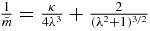 , and we obtain the following expression for u:

Using Mathematica, we plot in figure 21 the graph of 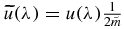 (which is what really defines the sign of u as a function of
 ![$\lambda \in [1, \sqrt{3}]$](https://content.cld.iop.org/journals/1751-8121/44/48/485204/revision1/jpa396475ieqn164.gif) since
since  ), and we clearly see that u is negative. Now, we can prove the following.

Figure 21. The function  for
for ![$\lambda \in [1,\sqrt{3}]$](https://content.cld.iop.org/journals/1751-8121/44/48/485204/revision1/jpa396475ieqn167.gif) .
.
Download figure:
Standard imageTheorem 4. In the planar RRFBP, the equilibrium solution (0, 0) is unstable in the Liapunov sense.
Proof. It is enough to observe that in this case, the eigenvalues of the linear part are given by the roots of the characteristic polynomial

with ρ = λ2 and u, v as in equation (57). The roots of p(ρ) are given by

By lemma 8, we know that u < 0 and then according to lemma 7, it follows that there exists at least one complex root of the characteristic polynomial in (53) with non-zero real part. Therefore, the conclusion follows.
Due to their specific location, we divide the equilibrium solutions into six groups: E0—the origin; Eξ(interior)—the non-zero equilibria located on the ξ-axis inside the rhombus configuration; Eξ(exterior)—the equilibria located on the ξ-axis outside the rhombus configuration; Eη—the non-zero equilibria located on the η-axis outside the rhombus configuration; Eint—the non-zero equilibria located off both axes and internal to the rhombus configuration; Eext—the non-zero equilibria located off both axes and external to the rhombus configuration. Although the previous result is general, we present individual numerical arguments to support the evidence in each case.
Figures 22–24 refer to the equilibria belonging to Eξ(interior), i.e. on the ξ-axis and inside the rhombus configuration. Remember that  . Δ > 0 if λ ∈ (λb, 1.254) and if
  . The pictures of ρ+ and of ρ− are obviously plotted in the two regions where Δ > 0.

Figure 22. The graphs of γ, Δ computed on the equilibria on the ξ-axis, inside the rhombus.
Download figure:
Standard image
Figure 23. The graphs of ρ+ where Δ > 0, computed on the equilibria on the ξ-axis, inside the rhombus.
Download figure:
Standard image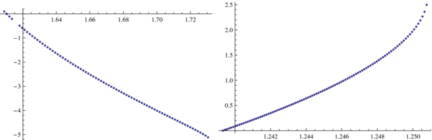
Figure 24. The graphs of ρ− where Δ > 0, computed on the equilibria on the ξ-axis, inside the rhombus.
Download figure:
Standard imageFigures 25 and 26 refer to the equilibria belonging to Eξ(exterior), i.e. on the ξ-axis and outside the rhombus configuration. We observe that γ < 0 if λ ∈ [1, 1.3147) and γ > 0 if  . Δ is an increasing positive function and Δ > 11.5435 for all values of λ. ρ+ is an increasing positive function and ρ+ > 3.188 49 for all values of λ.

Figure 25. The graphs of γ, Δ, computed on the equilibria on the ξ-axis, outside the rhombus.
Download figure:
Standard image
Figure 26. The graphs of ρ+ and ρ−, computed on the equilibria on the ξ-axis, outside the rhombus.
Download figure:
Standard imageFigures 27 and 28 refer to the equilibria belonging to Eη, that is, the vertical axis. Remember that they only exist outside the rhombus. We observe that γ < −0.2 for all values of ![$\lambda \in [1,\sqrt{3}]$](https://content.cld.iop.org/journals/1751-8121/44/48/485204/revision1/jpa396475ieqn171.gif) . Δ is a positive convex function and Δ > 8.5 for all values of λ. ρ+ is a positive convex function and ρ+ > 2.5 for all values of λ.
. Δ is a positive convex function and Δ > 8.5 for all values of λ. ρ+ is a positive convex function and ρ+ > 2.5 for all values of λ.

Figure 27. The graphs of γ, Δ, computed on the equilibria on the η-axis, outside the rhombus.
Download figure:
Standard image
Figure 28. The graphs of ρ+ and ρ−, computed on the equilibria on the η-axis, outside the rhombus.
Download figure:
Standard imageFigures 29 and 30 refer to the equilibria belonging to Eint. We observe that γ > 2 for all values of ![$\lambda \in [1,\sqrt{3}]$](https://content.cld.iop.org/journals/1751-8121/44/48/485204/revision1/jpa396475ieqn172.gif) . Δ is a positive decreasing function and Δ > 12 for all values of λ. ρ+ is a positive decreasing function and ρ+ > 6 for all values of λ.
. Δ is a positive decreasing function and Δ > 12 for all values of λ. ρ+ is a positive decreasing function and ρ+ > 6 for all values of λ.

Figure 29. The graphs of γ, Δ, computed on the equilibria off the axis, inside the rhombus.
Download figure:
Standard image
Figure 30. The graphs of ρ+ and ρ−, computed on the equilibria off the axis, inside the rhombus.
Download figure:
Standard imageFigure 31 refers to the equilibria belonging to Eext, i.e. off the axis and in the region external to the rhombus. We observe that γ is a negative increasing function and that γ < −0.24 for all values of ![$\lambda \in [1,\sqrt{3}]$](https://content.cld.iop.org/journals/1751-8121/44/48/485204/revision1/jpa396475ieqn173.gif) . Δ is a negative decreasing function and Δ < −10 for all values of λ. ρ+ and ρ− are not real-valued functions.
. Δ is a negative decreasing function and Δ < −10 for all values of λ. ρ+ and ρ− are not real-valued functions.
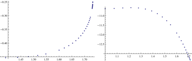
Figure 31. The graphs of γ, Δ, computed on the equilibria off the axis, outside the rhombus.
Download figure:
Standard imageIn table 2, we summarize all the results on the stability of the equilibrium solutions. We call λ1 = α1 + i β1,  and λ2 = α2 + i β2,
  , with
  , j ∈ {1, 2}, the four eigenvalues of the linearized problem at each equilibrium solution.
Table 2. Type of eigenvalues of each equilibrium point of the RRFBP, where  and
and  with j = 1, 2.
| λ1 | λ2 | |
|---|---|---|
The origin; ![$\lambda \in [1,\sqrt{3}]$](https://content.cld.iop.org/journals/1751-8121/44/48/485204/revision1/jpa396475ieqn179.gif) |
α1 + i β1 |  |
Eξ(interior);  |
α1 | i β2 |
| Eξ(interior); λ = 1.254 or λ = 1.584 | α1 |  |
| Eξ(interior); λ ∈ (1.254, 1.584) | α1 ± i β1 |  |
Eξ(exterior); ![$\lambda \in [1,\sqrt{3}]$](https://content.cld.iop.org/journals/1751-8121/44/48/485204/revision1/jpa396475ieqn184.gif) |
α1 | i β2 |
Eη ; ![$\lambda \in [1,\sqrt{3}]$](https://content.cld.iop.org/journals/1751-8121/44/48/485204/revision1/jpa396475ieqn185.gif) |
α1 | i β2 |
Einterior ; ![$\lambda \in [1,\sqrt{3}]$](https://content.cld.iop.org/journals/1751-8121/44/48/485204/revision1/jpa396475ieqn186.gif) |
α1 | i β2 |
Eexterior; ![$\lambda \in [1,\sqrt{3}]$](https://content.cld.iop.org/journals/1751-8121/44/48/485204/revision1/jpa396475ieqn187.gif) |
α1 + i β1 |  |
From numerical evidence and information contained in table 2, we have the following result.
Theorem 5. For any value of λ in the planar RRFBP, all the equilibrium solutions (ξ*, η*) are unstable in the Liapunov sense.
6.1. The symmetric case: the rhombus is a square
We consider the case κ = λ = 1 in which  . We know that λb > 1 and therefore there is no equilibria inside the square with η = 0, except for the origin. We find ξ*0 = 1.880 46. Also we observe that due to the symmetry of the square at the point (0, 1.880 46), we also have equilibrium.
We also know from [1] that in the square case, the other equilibria are at the line η = ξ. We find them to be ξ*i = 0.493 122 and ξ*e = 1.133 07. That is, one of them is inside and the other outside of the square, both on the mediatrix.
Table 3 summarizes our results.
Table 3. The eigenvalues in the square.
| ρ+ | ρ− | |
|---|---|---|
| (0, 1.8804) | 3.188 49 |  3.606 88 3.606 88 |
| (1.8804, 0) | 3.188 49 |  3.606 88 3.606 88 |
| (0.4931, 0.4931) | 19.5887 |  10.6964 10.6964 |
| (1.8804, 1.8804) |  0.444 437 + 3.260 48 i 0.444 437 + 3.260 48 i |
 0.444 437 −3.260 48 i 0.444 437 −3.260 48 i |
7. Periodic solutions via the Liapunov center theorem
In this section, we prove the existence of periodic solutions close to some equilibria. For ![$\lambda \in [1, \sqrt{3}]$](https://content.cld.iop.org/journals/1751-8121/44/48/485204/revision1/jpa396475ieqn195.gif) according to the previous sections, there are different equilibrium points and the eigenvalues of the linear part are given in table 2. In particular, we have one equilibrium point P1 = (ξ*, 0) (in the interior of the rhombus) on the ξ-axis at which for
according to the previous sections, there are different equilibrium points and the eigenvalues of the linear part are given in table 2. In particular, we have one equilibrium point P1 = (ξ*, 0) (in the interior of the rhombus) on the ξ-axis at which for  the associated eigenvalues satisfy
  and
and  . At the point P2 = (ξ*, 0) in the ξ-axis and outside of the rhombus for every value of
 ![$\lambda \in [1, \sqrt{3}]$](https://content.cld.iop.org/journals/1751-8121/44/48/485204/revision1/jpa396475ieqn199.gif) , the associated eigenvalues are
, the associated eigenvalues are 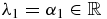 and
and  . The same behavior is obtained for the equilibrium point P3 = (0, η*) on the η-axis outside the rhombus and for the equilibrium point P4 = (ξ*, η*) inside the rhombus and not on the coordinates axis, for any value
 ![$\lambda \in [1, \sqrt{3}]$](https://content.cld.iop.org/journals/1751-8121/44/48/485204/revision1/jpa396475ieqn202.gif) .
.
Therefore, under the previous notation by the Liapunov center theorem (see theorem 9.2.1 of [3])), we obtain the following theorem.
Theorem 6. There are four one-parameter families of periodic orbits of the RRFBP emanating from each of the equilibrium points P1, P2, P3 and P4. Moreover, when approaching the equilibrium point along each family, the period tends to  .
.
8. Existence of transversal ejection-collision orbits and periodic solutions of long period
If m5 moves close to one of the positive masses, the gravitational field acting on it is due mostly to that mass, and orbits should look something like orbits of the two-body problem. Indeed, as the energy approaches minus infinity, the particles approach each other, and this corresponds to a singularity in the equations and the limit case corresponds to a double collision. It has long been known how to regularize this singularity, and we shall make use of the transformation due to Lévi-Cività for this purpose. First, we begin by considering the change of canonical coordinates given by

Thus, the Hamiltonian function (22) can be written as
where

Now, the binary collision between the bodies m1 and m5 in the new coordinates corresponds to the points x1 = 0 and x2 = 0. In our approach, we consider the regularization due to Lévi-Cività [6]. Position and momentum coordinates of m5 will be denoted, respectively, by the complex numbers

where i2 = −1. Hamiltonian (58) describing the motion is then written as

where

and

with w2 = −2λ, w3 = −λ + i and w4 = −λ − i.
Let us define  , where
  and we obtain the following Hamiltonian system:

with

where

From now on, we assume that m5 moves in the Hill region around m1 (around X0 = (x1, x2) = (0, 0)) and the energy is negatively large enough so that |X0| < 1/2 in this region. We suppose that the infinitesimal mass m5 rotates around the primary m1. With all these assumptions, now we expand this function in Taylor series and it yields

with  and
and  . Substituting this expansion into
  , the Hamiltonian can be written as

It is seen that the system has a singularity at z = 0, which corresponds to a collision of m1 and m5. This singularity is regularized by a transformation due to Lévi-Cività as follows: we define a small parameter ε as C = −1/ε2, restrict our attention to the energy surface H + 1/ε2 = 0 and introduce new variables (x, w) by a canonical transformation with a scaling of time

which we note is a double covering  identifying the pairs (x, w) and ( − x, −w), where
  . The resulting Hamiltonian is
We observe that the system

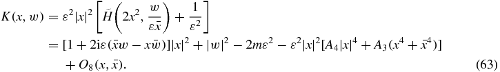
has an equilibrium point at x = w = 0. The restriction of the flow to K = 0 corresponds to the solutions of our problem. It is clear from (63) that if one disregards the last term of order 6 in  , we obtain the Kepler problem in rotating coordinates.
Theorem 7. For every λ and constant level C < 0 sufficiently negatively large, there exist an uncountable number of invariant punctured tori in the corresponding (non-compact) energy surface in the RRFBP. Moreover, the finitely many removed points of a punctured torus correspond to binary collisions with the primary m1.
Proof. The proof of this theorem follows the same spirit used for the planar circular restricted three-body problem in Conley's thesis [5] or in [4] for any values of the masses m,  and the shape of the rhombus. In fact, we point out that the terms of the Taylor expansion in the Hamiltonian K which are used during the proof are

where in the planar circular restricted three-body problem, A3 = 3 and A4 = 2, and μ and ν are changed to m and  , respectively. On the other hand, our problem also has the symmetry of reflection, see (23).
The proof is based on a comparison between Lévi-Cività and McGehee regularizing variables. The structure of K is good enough. If one keeps only the leading (quadratic) terms, the linear flow that one obtains (Hopf flow) is, up to the twofold covering, the usual regularization of the two-body problem by the geodesic flow on the round 2-sphere. If one ignores the last term ![$\varepsilon ^2 |x|^2[A_4 |x|^4+ A_3 (x^4+ \bar{x}^4)]$](https://content.cld.iop.org/journals/1751-8121/44/48/485204/revision1/jpa396475ieqn214.gif) (which is of order 6 in x), one obtains the still integrable two-body problem in a rotating frame: the complement in the energy surface of two linked periodic orbits (corresponding to the direct and retrograde circular motions having the given value of the Jacobi integral) is foliated by invariant tori parameterized by the angular momentum. The 'middle' torus, corresponding to zero angular momentum, contains the 'circle' x = 0 and each integral curve lying on this torus is made up of ejection–collision orbits. When the perturbation
(which is of order 6 in x), one obtains the still integrable two-body problem in a rotating frame: the complement in the energy surface of two linked periodic orbits (corresponding to the direct and retrograde circular motions having the given value of the Jacobi integral) is foliated by invariant tori parameterized by the angular momentum. The 'middle' torus, corresponding to zero angular momentum, contains the 'circle' x = 0 and each integral curve lying on this torus is made up of ejection–collision orbits. When the perturbation ![$\varepsilon ^2 |x|^2[A_4 |x|^4+ A_3 (x^4+ \bar{x}^4)]$](https://content.cld.iop.org/journals/1751-8121/44/48/485204/revision1/jpa396475ieqn215.gif) is added, the two periodic orbits associated with circular movements continue to exist: they now correspond to quasi-circular direct and retrograde motions of the zero-mass body in the rotating frame. As in [5] or [4], one can take these orbits as the boundary of an annulus of section; moreover, one can choose this annulus in such a way to contain the 'circle' x = 0. The results are stated in terms of the Poincaré first return map Pε on such an annulus
is added, the two periodic orbits associated with circular movements continue to exist: they now correspond to quasi-circular direct and retrograde motions of the zero-mass body in the rotating frame. As in [5] or [4], one can take these orbits as the boundary of an annulus of section; moreover, one can choose this annulus in such a way to contain the 'circle' x = 0. The results are stated in terms of the Poincaré first return map Pε on such an annulus  . The existence of transversal ejection–collision orbits in the RRFBP is shown to imply, via KAM theorem, the existence, for C < 0 large enough, of an uncountable number of invariant punctured tori in the corresponding energy surface.
Another important consequence follows from the fact that the collection of fixed points of iterates Pε is infinite; these fixed points correspond to the long periodic solutions of the RRFBP. Since the same arguments are valid in any neighborhood of each binary collision, we have proved the following.
Corollary 1. For every λ and level constant C < 0 sufficiently large, there exist periodic solutions of long period for the RRFBP which are close of each binary collision.
9. Summary of results
We have obtained the first integral of motion. The Hamiltonian function which governs the motion of the fifth mass is obtained and has two degrees of freedom depending periodically on time. We use a synodical system of coordinates to eliminate the time dependence. With the help of the Hamiltonian structure, we characterize the regions of possible motion. We show the existence of equilibrium solutions along the coordinate axis as well as off of them. We verify that the number of equilibrium depends on λ and there can be 11, 13 or 15 equilibrium solutions, all unstable. We prove the existence of periodic solutions with short as well as long periods. Also we prove the existence of transversal ejection–collision orbits (binary collisions) for certain large values of the Jacobi constant, for an uncountable number of invariant punctured tori in the corresponding energy surface.
Acknowledgment
The authors were partially supported by Regional Program MATH-AmSud 2009.