Abstract
The Python libraries NumPy and SciPy are extremely powerful tools for numerical processing and analysis well suited to a large variety of applications. We developed ObsPy (http://obspy.org), a Python library for seismology intended to facilitate the development of seismological software packages and workflows, to utilize these abilities and provide a bridge for seismology into the larger scientific Python ecosystem. Scientists in many domains who wish to convert their existing tools and applications to take advantage of a platform like the one Python provides are confronted with several hurdles such as special file formats, unknown terminology, and no suitable replacement for a non-trivial piece of software. We present an approach to implement a domain-specific time series library on top of the scientific NumPy stack. In so doing, we show a realization of an abstract internal representation of time series data permitting I/O support for a diverse collection of file formats. Then we detail the integration and repurposing of well established legacy codes, enabling them to be used in modern workflows composed in Python. Finally we present a case study on how to integrate research code into ObsPy, opening it to the broader community. While the implementations presented in this work are specific to seismology, many of the described concepts and abstractions are directly applicable to other sciences, especially to those with an emphasis on time series analysis.
Export citation and abstract BibTeX RIS
1. Introduction
The scientific Python ecosystem built around NumPy [23] and SciPy offers a wealth of possibilities for all fields of science, mathematics, and engineering. This enables the creation of versatile and powerful workflows and applications. Over the years many fields of science have developed their own set of file formats, tools and analysis software adapted to suit their particular tasks and attempting to extend these to more flexible uses often ends up being hard or impossible. Therefore a more general approach like the one offered by the SciPy stack (http://scipy.org/stackspec.html) is desirable.
ObsPy [2] provides read and write support for essentially all file formats commonly distributed within the seismological community superseding an abundance of file format converters. On top of this broad I/O support it offers signal processing routines utilizing a jargon prevailing among seismologists. A third milestone is the integrated access to data distributed by a wide range of seismic data centers worldwide and finally, it integrates a number of special purpose libraries in use in seismology while unifying all functionality with an easy to use interface.
2. Domain-specific time series analysis
The ObsPy library contains a domain-specific time series analysis toolkit which enables seismologists to construct processing workflows in a notation familiar to them. It thus provides an interface to the vast functionality offered by NumPy and SciPy to domain experts which might otherwise hesitate to invest into learning Python and its scientific ecosystem. The first section contains a technical description of how a number of different time series file formats can be handled in a unified manner and how to use a plug-in system to map general signal processing routines provided by NumPy and SciPy to the aforementioned convenient interface. This approach has proven itself to work very well and we believe it can easily be applied to other fields.
2.1. Seismic waveforms
Seismology is the study of the propagation of elastic waves through mostly solid media. The seismic waves result from natural (tectonic earthquakes, volcanoes, ocean waves) or man-made (nuclear explosions, quarry blasts, induced earthquakes) sources and are measured and recorded at seismographs. These perform point measurements of the elastic wavefield in up to three orthogonal directions. Each direction or component measures either the displacement, velocity or acceleration of the ground motion in the form of a one-dimensional, time-dependent signal. The resulting equally sampled time series are called seismograms or seismic waveforms.
With the emergence of digital seismology in the last couple of decades, numerous seismic waveform file formats have surfaced. Some, like the MiniSEED format [18] for data archiving and streaming, were designed with a specific purpose in mind, while the majority of formats are by-products of seismic signal processing or analysis packages that used custom formats for their I/O. The adoption of some of these software packages caused their I/O formats to become widely used data exchange formats—a purpose for which they were not designed. A recurring problem, for example, is the byte ordering: most formats do not specify whether they are written in big or little endian and for many formats, examples of both can be found. This myriad of file formats and software suites only accepting one particular file format caused many format converters to be written and distributed.
Each available waveform format in essence stores one or more time series and some meta-information about it. The essential ingredients of these formats can be distilled to a common subset of information enabling the use of a unified internal representation. ObsPy provides an implementation of that idea, which is described in the following section.
2.2. Characteristics of waveform data formats
Assuming that a seismic data recording starts at time A, ends at time B and is equidistantly sampled without gaps and overlaps, it can be uniquely described by the time of the first sample, the sampling rate, the instrument it was recorded with and an array containing the signal. This is the common core information and all waveform file formats have to contain it in some fashion. In seismology receivers are uniquely identified by the so-called SEED identifiers [18] consisting of four short strings. A globally coordinated effort attempts to ensure that this system stays intact and as a direct result, most waveform formats adhere to it, offering a solution to the receiver location issue.
Seismic data also often have gaps and overlaps meaning that the data is not evenly sampled and the previous assumption does not hold true anymore. Gaps can result from short losses of power at the recording station or problems with the data transfer. Clock drifts and corrections can be one of the reason for the overlap of data points. Some data formats and ObsPy deal with this by allowing the storage of multiple chunks of waveform data, each being equally sampled and generally well behaved in itself.
Any additional information a waveform file format might support within ObsPy is stored separately as detailed in the next section.
2.3. Internal data representation
Within ObsPy, waveform data are represented by a Stream object that acts as a container for any number of Trace objects. ObsPy defines a Trace to contain a single, contiguous, equally sampled time window of waveform data alongside the necessary meta-information. Each Trace object has a data attribute, which is a one-dimensional NumPy array. All further information is located in the dictionary-like stats attribute.
The stats object stores the four SEED identifiers network, station, location and channel, denoting the recording's physical location and instrument. It furthermore contains the times of the first and last sample, the data's sampling rate and interval and the number of samples. This information is partially redundant and ObsPy takes care that it stays consistent. For example, the endtime attribute is read-only and will be adjusted automatically if the start time, the sampling rate or the number of samples in the array has changed. Any additional information a specific file format might contain not covered by this abstraction will be stored in a container inside the stats object. See figure 1 for an illustration of the described internal representation.
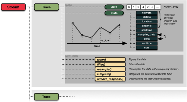
Figure 1. Illustration of ObsPy's internal waveform data representation in the form of the Trace objects gathered in a Stream object. Each Trace object represents a contiguous, equally sampled time series with the samples stored in a NumPy array; additional metadata are placed under the stats attribute. The Stats object will keep the meta-information self-consistent by making use of custom item setters. A collection of domain-specific signal processing methods enables scientists to construct workflows in a terminology with which they are familiar.
Download figure:
Standard image High-resolution image2.4. Broad data format support by means of a plug-in system
In order to support as many waveform file formats as feasible, a modular plug-in approach has been chosen with each supported data format being its own submodule and registering with ObsPy with the help of pkg-util's plug-in system. Listing 1 shows the registration of an example waveform plug-in. A file format submodule has to implement two functions with specified interfaces, and a third one is optional:
- is_format(filename): format identification function. Returns True if the passed file is of the submodule's format; False otherwise.
- read_format(filename, ∗∗kwargs): reads the file and returns a Stream object containing a representation of the file's data.
- write_format(stream, filename, ∗∗kwargs): writes a Stream object to the given filename; this function is optional, and if not given, no write support for the format will be available.
Listing 1:. excerpt from ObsPy's setup.py script demonstrating how the waveform plug-in entry points are defined on the example of the MiniSEED plugin. distutils will then take care of registering the plug-in upon installation. Other Python modules can register their own waveform format plug-ins for rarely used formats.
| ENTRY_POINTS={ |
| ... |
| "obspy.plugin.waveform": [ |
| ... |
| "MSEED = obspy.mseed.core", |
| ... |
| ] |
| ... |
| "obspy.plugin.waveform.MSEED": [ |
| "isFormat = obspy.mseed.core:isMSEED", |
| "readFormat = obspy.mseed.core:readMSEED", |
| "writeFormat = obspy.mseed.core:writeMSEED", |
| ], |
| ... |
| } |
The forced modularity of this strategy fosters a clean separation of concerns with each submodule being implemented and tested independently. In addition, it allows users to extend ObsPy with I/O support for formats that are not used widely enough to justify integration into the main ObsPy library. A common example for this is output formats of numerical waveform solvers. pkg-utils' plug-in system will register these additional formats for a seamless integration with the rest of ObsPy.
2.5. Format autodetection and usage
ObsPy comes with a top-level read() function, a single entry point when reading waveform data. See the listing 2 for a usage example.
Listing 2:. snapshot of an interactive Python session demonstrating the usage of ObsPy's read() function. It will detect the file's format and call the appropriate reading routine. In case the read() routine detects a valid HTTP URL it will download the resource before proceeding. In case it detects an archive format it will be decompressed first.
| >>> import obspy |
| >>> st=obspy.read("filename") |
| >>> st |
 obspy.core.stream.Stream at 0x2f284d0
|
| >>> print st |
| 3 Trace(s) in Stream: |
BW.RJOB..EHZ  2009--08-24T00:20:03.000000 Z -... 2009--08-24T00:20:03.000000 Z -...  100.0 Hz, 3000 samples 100.0 Hz, 3000 samples
|
BW.RJOB..EHN  2009--08-24T00:20:03.000000 Z -... 2009--08-24T00:20:03.000000 Z -...  100.0 Hz, 3000 samples 100.0 Hz, 3000 samples
|
BW.RJOB..EHE  2009--08-24T00:20:03.000000 Z -... 2009--08-24T00:20:03.000000 Z -...  100.0 Hz, 3000 samples 100.0 Hz, 3000 samples
|
The read(filename, ∗∗kwargs) routine calls all registered formats' is_fileformat() functions until one returns True. Depending on the format in question the is_fileformat() routine parses the first couple of bytes or performs more complicated heuristics. For performance reasons the format detection routines have to be fast. On top of that, ObsPy performs the format detection according to a manually curated list so that the most commonly used ones are tested first, improving average performance. After the format has been determined the appropriate format's read_fileformat() function will be called, which parses the file and returns a Stream object. The format detection can also be skipped by providing the format to the read() routine.
This structure permits the sharing of capabilities among all formats by implementing them as part of the read() routine. Examples of this are automatic file downloading if a valid HTTP URL is detected and the decompression of a number of different archive formats.
Web services provided by data centers around the globe are an important source for waveform data. ObsPy implements clients able to interact with a comprehensive selection of such data centers [20]. A waveform data request will end up being stored in a Stream object so the workflow following the data acquisition is identical no matter the origin of the data.
2.6. Domain-specific convenience methods
A unified internal data representation opens the possibility of defining methods transforming it. With respect to this, ObsPy offers a comprehensive collection of signal processing routines frequently used in seismology by relying heavily on functionality coming with NumPy and SciPy. These are implemented to match the needs seismologists have for a certain processing operation while keeping the data self-consistent. An example of this is the Trace.decimate() method which will apply a filter, decimate the data and adjust the sampling rate metadata of the times series. Caused by the potentially large number of samples, most operations are implemented as in-place modifications of the Stream and Trace objects.
Most processing methods are defined on a single Trace; the same methods on the Stream objects will call the corresponding method on each of their Trace children. This allows for a natural handling of three and more component data. A number of methods are specific to Stream methods. Consult table 1 for a selection of available signal processing routines.
Table 1. Selection of processing methods for the Stream and Trace objects. Most Trace methods are also available on the Stream objects which will apply the chosen method to all their children.
| Stream methods | ||
|---|---|---|
| merge() | Attempts to merge Trace objects with the same ID | |
| rotate() | Rotates two- or three-component Stream objects | |
| select() | Returns a new Stream with Traces matching the selection | |
| Trace methods | ||
| decimate() | Decimates the data by an integer factor | |
| detrend() | Removes a linear trend from the data | |
| differentiate() | Differentiates the data with respect to time | |
| filter() | Filters the data | |
| integrate() | Integrates the data with respect to time | |
| normalize() | Normalizes the data to its absolute maximum | |
| remove_response() | Deconvolves the instrument response | |
| resample() | Resamples the data in the frequency domain | |
| taper() | Tapers the data | |
| trigger() | Runs a triggering algorithm on the data | |
| trim() | Cuts the data to given start and end time |
In order to offer a large variety of functionality, ObsPy once again employs a plug-in system. Listings 3–5 demonstrate this by example with the Trace.taper() method. The employed plug-in system empowers the usage of functionality defined by different modules into a simple domain-specific API usable by scientists. It furthermore encourages code deduplication and reuse and thus enables ObsPy to offer a large variety of different functions without having to implement and test the details in many cases.
Listing 3:. excerpt from ObsPy's setup.py file. Upon installation these entry points will be registered and made available to pkg-utils. The code snippet illustrates this by registering different taper windows. At the time of writing ObsPy exposes 18 different taper windows mainly from the scipy.signal module. Usage is demonstrated in the listing 5.
| ... |
| "obspy.plugin.taper": [ |
| "cosine = obspy.signal.invsim:cosTaper", |
| "barthann = scipy.signal:barthann", |
| ... |
| ] |
| ... |
Listing 4:. code fragments from within the Trace object's taper() method. It shows how the functions registered as illustrated in the listing 3 are called to obtain different taper windows and how optional keyword arguments are passed to it. Usage is demonstrated in the listing 5.
| ... |
| # retrieve function call from entry points |
| func = _getFunctionFromEntryPoint( |
| "taper", type) |
| ... |
| taper_sides = func(2 ∗wlen, ∗∗kwargs) |
| ... |
Listing 5:. usage of the functions registered and called in listings 3 and 4. Note how the actual taper windows can be and in this case are defined in different Python modules. On top of that, this listing demonstrates method chaining which is possible because the methods return their objects. The calls to copy() are necessary as most methods work in place and therefore would modify the object. This memory-saving behavior is wanted in most cases and is a conscious design choice to match the average use case.
| import obspy |
| st = obspy.read("filename") |
| # Taper with a cosine window. |
| st2 = st.copy().taper("cosine") |
| # Taper a with modified Bartlett-Hann window. |
| st3 = st.copy().taper("barthann") |
| # The methods can be chained for a compact notation. |
| st4 = st.copy().detrend("linear").taper("cosine") |
3. Integration of legacy codes
For certain tasks the seismological community frequently relies on codes that have been in use for a decade or more. This heavy exposure and application to a large variety of problems assures that they work as expected in almost all cases as most issues have already been discovered and fixed. While these codes are often cumbersome to use, it is desirable to keep them vivid and to profit from the investment made in their development in the past. ObsPy integrates a number of legacy codes, enabling the use of modern workflows and recent advances in data processing while simultaneously relying on stable and well tested code for a specific functionality. This section illustrates this on two examples.
3.1. Travel time calculations with iaspei-tau
The calculation of seismic travel times is a problem frequently encountered in seismology. If an earthquake occurs at point X the question is what seismic phases arrive at what time at point Y. The cost for full 3D simulations of the whole Earth [29] are excessive for many applications and less accurate but faster approximations are often sufficient. In case a 1D spherically symmetric Earth model is applicable, the frequently used method of Buland and Chapman [3] enables very fast travel time calculations. It has been implemented in a Fortran package commonly called iaspei-tau [14, 26]. A more feature-rich Java version of this algorithm is also available [4]. The obspy.taup submodule uses ctypes from the Python standard library to provide a pythonic interface to iaspei-tau; see the listing 6. Figure 2 plots the travel times of an earthquake through the Earth versus the geographic distance in degrees.
Listing 6:. usage of obspy.taup to attain travel times for seismic phases originating from a source with a distance of 25° and a depth of 10 km. The distance delta is given in degrees assuming a spherical Earth, the depth is in kilometers and the Earth model is ak135. It returns a list instead of a dictionary as the phase names are non-unique for certain distance and phase combinations.
| >>> from obspy.taup import getTravelTimes |
| >>> getTravelTimes(delta=25.0, depth=10.0, model="ak135") |
| [{"phase_name": "P", |
| "take-off angle": 28.375334, |
| "time": 323.91006, ...}, |
| {"phase_name": "pP", |
| "take-off angle": 151.61096, |
| "time": 326.94455, ...}, |
| ... |

Figure 2. Travel times of seismic waves through the 1D Earth model ak135. The top graph shows travel times for some seismic phases calculated by the obspy.taup module. The bottom plot shows the difference for the P phase travel times calculated with the TauP Toolkit [4] and obspy.taup. The deviations are mainly due to differing internal coordinate systems and are well understood by the community [15]. The amplitude of the differences strongly depends on the used seismic phase and the source-receiver geometry.
Download figure:
Standard image High-resolution image3.2. Instrument responses: Stationxml harnesses evalresp
Seismic receivers distributed around the globe aim to measure and record ground motion as accurately as possible. Many factors influence the characteristics of the final waveform, among them the frequency response of the physical instrument, the effects of any amplifiers, of analog and digital filters and of the digitalization. For many applications studying the Earth, it is crucial to eliminate these effects to get the best possible estimate of the true ground motion. The first step when correcting data for the influence of the seismic receiver and processing chain is to calculate the frequency response of the recording system. The seismograms are then deconvolved with this response to obtain a seismogram with physical units unbiased by instrumental effects in the frequency band of consideration. This process is known as instrument correction in seismology.
Listing 7:. C struct representing the physical response of an instrument in form of poles and zeros. Recreating this with ctypes requires the definition of a Python class which is shown in the listing 8.
| struct complex { |
| double real; |
| double imag; |
| }; |
| struct pole_zeroType { |
| int nzeros; |
| int npoles; |
| double a0; |
| double a0_freq; |
| struct complex *zeros; |
| struct complex *poles; |
| }; |
Listing 8:. Python class representing the pole_zeroType C structure shown in listing 7 using the ctypes library. complex_number is already defined in this example.
| import ctypes as C |
| ... |
| class pole_zeroType (C.Structure): |
| _fields_ = [ |
| ("nzeros", C.c_int), |
| ("npoles", C.c_int), |
| ("a0", C.c_double), |
| ("a0_freq", C.c_double), |
| ("zeros", C.POINTER(complex_number)), |
| ("poles", C.POINTER(complex_number)), |
| ] |
Seismic recording systems are described by a linear chain of different stages or elements. The SEED data format [18] accurately represents these, is widely accepted by the community and has been in use since the early 1990s. Recently, StationXML [19], the designated successor of SEED, was developed, and the community is starting to adopt it. Being an XML format, it has many benefits in comparison to the binary SEED format regarding tool support, ease of data distribution and human readability. Except for some minor differences, both formats store the same information.
The standard workflow for calculating the frequency response of a seismic receiver system from SEED files involves rdseed [12] to generate RESP files, a textual strict subset of SEED. These files are then fed into evalresp [11] resulting in the frequency response. The detour via the RESP files is necessary as it is the only input file format evalresp accepts. Performing an instrument correction with metadata stored in StationXML files involves one additional step—the conversion of the StationXML files to SEED files using yet another tool.
Conducting this in Python involves a number of system calls and unnecessary I/O operations making it ill-suited to modern large data workflows. Replacing evalresp would be a major effort as many pitfalls exist when calculating instrument responses, which can greatly influence the final result. Instead ObsPy offers a direct bridge from StationXML (parsed through lxml) to evalresp utilizing ctypes to call internal evalresp functions. This approach is not feasible for code that is still actively developed as no guarantees on the stability of the internal API are usually granted. However, evalresp is not in active development anymore and only receives an occasional maintenance commit.
ObsPy's internal representation of StationXML data is used to derive the nested C structures evalresp's internal functions expect. These are defined and initialized using ctypes as demonstrated in listings 7 and 8. Ctypes also requires a definition of the function headers as shown in listings 9 and 10. Figure 3 displays the amplitude and phase response calculated from a StationXML file also illustrating the effect of different stages in the recording system.

Figure 3. Amplitude and phase response of channel XM.05..HHZ to convert a seismogram from m s−1 to digital counts. The recording instrument is a Guralp CMG-6TD seismometer. The green line shows the response if only the physical instrument and the gain from the analog to digital converter are taken into account. The black line also incorporates the three successive digital decimation stages, and the red line is the Nyquist frequency for this particular channel. The green and black lines have been calculated using ObsPy's integration of evalresp. For comparison, the orange line shows the results for the same calculation performed by JEvalResp [13], a Java port of evalresp and one of the very few software packages able to perform this calculation. The agreement is very good; the differences after the Nyquist frequency are due to the spacing of the discrete frequency values needed for plotting.
Download figure:
Standard image High-resolution imageA seismic receiver's recording system usually has several stages resulting in a fairly complex representation within evalresp. Evalresp's file parsing stage takes care of translating the SEED constructs to the appropriate internal structure and sometimes makes non-obvious decisions. To ensure the correctness of the evalresp integration we performed an extensive test [16]. We define our integration of evalresp acting on StationXML files to be correct if the final response is equivalent to a response calculated by converting StationXML to SEED and SEED to RESP files on which evalresp is acting. We downloaded almost the complete set of StationXML inventory data available from IRIS, the largest data distributor in seismology. Data from over 27 000 stations, most with multiple recording channels defined for different periods in time result in well over 100 000 instrument responses. We reiterated our implementation until the tests passed, giving confidence that our solution can be safely applied to any data encountered in the world wide community.
Listing 9:. function declaration in the C code of evalresp. This is the main function used to calculate the response. Note how the input takes a number of different parameters from simple integers to arrays of custom structs. The complex struct does not need to be defined on the Python side as the numpy.complex128 dtype does have the same internal memory layout.
| ... |
| struct complex { |
| double real; |
| double imag; |
| }; |
| ... |
| void calc_resp(struct channel ∗chan, |
| double ∗freq, |
| int nfreqs, |
| struct complex ∗output, |
| char ∗out_units, |
| int start_stage, |
| int stop_stage, |
| int useTotalSensitivityFlag); |
Listing 10:. the corresponding declaration to listing 9 in ctypes. The numpy.ctypeslib module provides array types that will result in automatic type, dimension and flag checks upon function invocation. This results in a convenient calling syntax and error handling on the Python side before calling the shared library.
| from obspy.signal.headers import clibevresp import ctypes as C |
| ... |
| clibevresp.calc_resp.argtypes = [ |
| C.POINTER(channel), |
| np.ctypeslib.ndpointer( |
| dtype='float64', ndim=1, |
| flags='C_CONTIGUOUS'), |
| C.c_int, |
| np.ctypeslib.ndpointer( |
| dtype='complex128', ndim=1, |
| flags='C_CONTIGUOUS'), |
| C.c_char_p, C.c_int, C.c_int, |
| C.c_int] |
| clibevresp.calc_resp.restype = C.c_void_p |
4. Integrating research code into ObsPy
4.1. Purpose
Contrary to the well-established, virtually bug-free legacy codes described above, many scientists using Python in their analytic workflow tend to develop bits and pieces of codes that are applied to their input data, and thus at first sight not useful for others. This general ascertainment is also true in seismology where input data can have different formats, outputs need to be compatible with different downstream processing software and so forth. In this section, we first present a case study of the translation of a C code that can read an exotic format called Win and then present a research code developed during a PhD thesis that is now integrated in ObsPy as a new module. Thanks to the pluggability of ObsPy, only the necessary processing steps need to be written.
4.2. Reading an excotic format—obspy.win
WIN is the format imagined by a Japanese company named Hakusan as default storage for their Datamark datalogger series. The data within a one-minute WIN file is highly compressed, every second being compressed with a different level from the previous. Up to now, there were three ways to convert WIN to a more standard format, namely SAC: Win2Sac and japan2sac in Linux and Win2Sac GUI on Windows. Win2Sac codes come from Japan, while the japan2sac was written as part of a research project in Chambery (France) and is not completely finished. In order to process these data using state of the art routines and software, e.g. using ObsPy-based scripts, one has to convert the whole archive to SAC, which is readable by ObsPy. Each step of this process doubles the volume of the archives stored on disk, and potentially adds errors to the final product.
Thankfully, sources of Win2Sac are available online [22] and together with the datasheet [30] describing the WIN format, we have been able to write an ObsPy plug-in to read it. The final goal was to be able to read directly from the archive without duplication and process those data the same way as data originating from other file formats. Even if one's goal is to convert WIN to MiniSEED, the best solution today will be to write a Python script using ObsPy and no longer rely on a succession of steps.
4.3. Rewriting research code to an ObsPy extension
The state of a volcano and its unrests can be evidenced by the amount of amplitude (or energy) recorded by seismic sensors on its flanks. Real-time seismic amplitude measurement (RSAM (1)) was initially introduced by Endo and Murray [8] to forecast eruptions and assess the state of volcanic activity. One can also compute the standard deviation of the squared amplitudes, or real-time seismic energy measurement (RSEM (2)) [5], of the signals over a certain time interval divided by the number of measurements.

where Ai is the seismic signal's amplitude, Aavg is the average over N samples.
As multiple sources are overlapping, volcano-seismologists typically calculate the RSEM or RSAM values for separate, previously defined frequency bands (spectral seismic energy measurement (SSEM) [28], similar to SSAM introduced by Stephens [27]. The data are first demeaned and bandpass filtered with a Butterworth filter of order two. Each value is then calculated on a 30 s window (100 × 30 samples). Finally, the daily 10th and 25th percentiles and the median are typically computed to partially remove undesired transients and earthquakes which are considered a disturbance of the tremor data [7].
The RSAM, RSEM, SSAM and SSEM algorithms have been implemented in the obspy.signal.ssxm submodule. The final code takes advantage of the resampling abilities of Pandas (Python Data Analysis Library), resulting in a total of less then 50 lines of code for the ssxm() method.
4.3.1. Example results
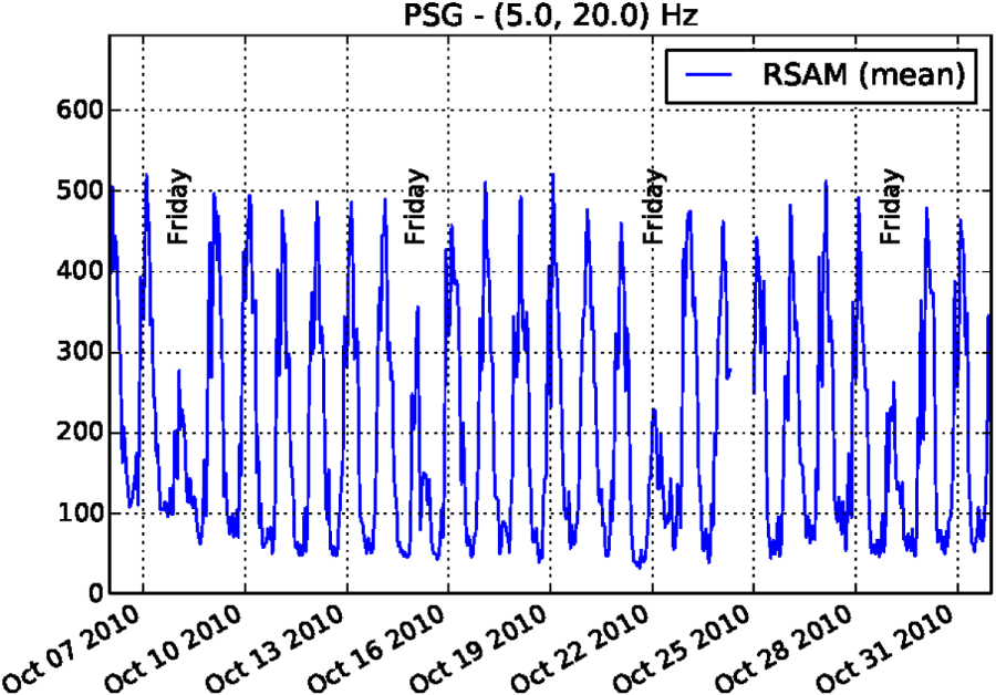
The interest of filtering the signal in different frequency bands can be illustrated with the Kawah Ijen volcano (East Java, Indonesia) seismic data. The seismic time series are generally polluted by anthropic activities during the day, especially in high frequency bands ( 10 Hz) and particularly for the stations located closer to the source of 'cultural' noise, in this case the parking and base camp for climbing the volcano. One may even observe weakened working activity during the prayer day (i.e. Friday, see figure 4). To minimize the effects of transients, one can use the 10th percentile (p10) of the amplitude in a specific frequency band (figure 5). Except during volcanic unrest (figure 5), the p10 data from station PSG are still highly affected by this anthropic noise, compared to POS and PUN, which are located around the crater, thus further away from the human activity.

Figure 4. Daily and weekly fluctuations of the seismic amplitude (RSAM) in the 5–20 Hz frequency band for station PSG during a quiet period of volcanic activity. Fridays (prayer day) are clearly visible. The amplitude is in counts.
Download figure:
Standard image High-resolution image
Figure 5. Transition between a period of unrest to a more quiet period of volcanic activity for stations around the crater (POS and PUN) and close to the parking/base camp for climbing the volcano (PSG). The anthropic influence is still visible on PSG even when computing the 10th percentile of the amplitude of the records.
Download figure:
Standard image High-resolution image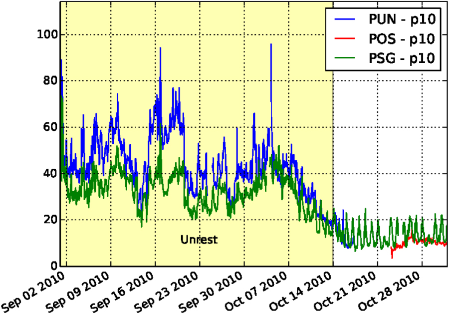
Other studies investigated some particular processes by filtering the seismic signal. For example, SSEM computations might provide a measure of the rate of strain released, if persistent fracturing at any scale produces a sustained seismic signal [6]. One can also assess the stationarity of the microseism noise sources (0.1–1 Hz) to evaluate the results from the velocity variations using ambient seismic noise cross correlation techniques [17].
5. Conclusion
Legacy codes and data formats are widely used in a number of sciences and will continue to play an important role in the foreseeable future. The approaches we laid out in this article help in integrating them in modern computing environments. Most of the illustrated design and implementation choices are transferable to other fields in computational science. The extraction of common features from a heterogeneous set of file formats enables the construction of data source independent workflows, which especially benefits data heavy domains. This, together with a library of functionality in a domain-specific vocabulary and the inclusion of some critical legacy codes, yields an attractive package even for users not familiar with Python.
ObsPy enjoys a large rate of adaption within the seismological community. We believe this is in large part due to it solving an actual problem: the various different file formats that previously required a plethora of file format converters or different signal processing tools. Once people start to use it they quickly discover the flexibility and power of Python. In contrast to, for example, MATLAB, using ObsPy also grants the advantages of a full-blown programming language. A further competitive edge is the many 3rd party modules in Python which are not directly associated with signal processing, enabling the use of, for example, databases, web services, machine learning libraries and of course, the recent developments in handling big data sets, which will become more and more important in seismology and other fields. On top of all that, the complete stack is free, open-source and runs on virtually every platform of relevance.
Studies that successfully utilized ObsPy include event relocations [21], rotational [10] and time-dependent [24] seismology, big data processing [1], and synthetic studies about full-waveform inversions [25] and attenuation kernels [9] to name a few examples. The ObsPy website, accessible under http://www.obspy.org contains detailed documentation, an extensive tutorial, and access to a mailing list in order to ease the transition to ObsPy and build a community around it. The modularity described in this manuscript and the test-driven development facilitate the addition of new functionality and as a result, ObsPy steadily increases the number of external contributions with the goal of becoming a code maintained by people throughout the community.
Acknowledgments
We want to thank the steadily growing ObsPy community for the continuous support and constant encouragement and exchange. By now, too many people contributed code and ideas to ObsPy to list them all, but we are grateful for each and every one of them. We also thank the developers of Python, NumPy and consorts, and the authors of a number of libraries integrated into ObsPy. Two anonymous reviewers helped to improve the final manuscript with thoughtful reviews.