
Abstract
Summer (June–July–August; JJA) UK precipitation extremes projections from two UK Met Office high-resolution (12 km and 1.5 km) regional climate models (RCMs) are shown to be resolution dependent. The 1.5 km RCM projects a uniform ( ) increase in 1 h JJA precipitation intensities across a range of return periods. The 12 km RCM, in contrast, projects decreases in short return period (≦̸5 years) events but strong increases in long return period (⩾20 years) events. We have low physical and statistical confidence in the 12 km RCM projections for longer return periods. Both models show evidence for longer dry periods between events. In winter (December–January–February; DJF), the models show larger return level increases (⩾40%). Both DJF projections are consistent with results from previous work based on coarser resolution models.
Export citation and abstract BibTeX RIS

Content from this work may be used under the terms of the Creative Commons Attribution 3.0 licence. Any further distribution of this work must maintain attribution to the author(s) and the title of the work, journal citation and DOI.
1. Introduction
Regional climate models (RCMs) have long been used to project future changes in precipitation [1]. The United Kingdom Met Office (UKMO) has recently completed a series of high-resolution (12 km and 1.5 km) RCM simulations [2, 3]. These resolutions are higher than previous studies [1] with the important feature that the latter uses no convective parameterisation ('explicit convection'). The simulations are run continuously over multiple years in order to produce consistent land surface feedbacks to the model-simulated climate. The 1.5 km grid boxes can resolve 'larger' moist convection (say storms that are 10 km wide) over the UK, but are still too coarse to resolve smaller showers; therefore, our explicit-convection 1.5 km model is often referred to as 'convective permitting' [2]. Convective permitting simulations have been shown to add value over parameterised convection simulations [2, 4]. We examined the extreme events in the reanalysis downscaling simulations [5]. Here we seek to expand on that work by examining the climate change signals for 1 h and 1 day precipitation extremes projected by the same two RCMs.
Simulations where the 1.5 km and 12 km RCMs have been driven by the ERA-interim reanalysis [6] have been extensively analysed [2, 5, 7]. The 12 km RCM has lower mean precipitation biases than the 1.5 km RCM, but performs poorly for hourly rainfall characteristics (such as precipitation duration and diurnal variability) and extreme measures (producing physically implausible large extremes for high return periods). Overall, we have lower confidence in the physical basis for the 12 km RCMʼs highest summer precipitation intensities [7], and we believe that the 12 km 'gray-zone'5 resolution is partially responsible for our concerns [5, 8].
Previous RCM extreme projections have mainly used lower-resolution models with convective parameterisations. These show relatively consistent projections for changes in winter extremes but large uncertainty in summer changes. For example, the 50 km UKMO RCM simulations projected a 10% increase in UK daily precipitation extremes [9]. No clear changes for future London daily precipitation extremes are found in the UKCP09 RCM ensembles [10]. 25 km ENSEMBLES multi-model projections [11] gave a  intensification of annual maximum hourly and daily precipitation for the Netherlands [12]. The Dutch RACMO 25 km RCM [13] projected an intensification of summer and winter daily extremes for the Rhine basin [14]. Regional signals for extreme summer daily precipitation change, as given by the 25 km ENSEMBLES multi-model projections, were found to be unlikely to emerge in this century across parts of Northern and Central Europe (including the southern UK), but winter signals are expected to emerge sooner [15]. In general, winter projections are more robust and consistent across models than summer projections [1].
The objective here is to examine projections for even higher resolution RCMs. Based on the above discussion, we expect the climate change projections for extreme precipitation to be substantially different between the two RCMs. In addition, we will highlight the importance of dry periods in extreme precipitation projections.
2. Model and observations
The 12 km and 1.5 km RCMs are fully described in previous papers [2, 3]. The 12 km RCM domain covers Europe and North Africa, and is driven by either the ERA-Interim reanalysis [6] or 60 km HadGEM3 present-day/future-climate general circulation model (GCM) simulations [16]. The 1.5 km RCM simulation spans the southern UK, and is a one-way nest down from the 12 km simulation. The 1.5 km RCM is based on the UKMO operational United Kingdom Variable forecast model. The 12 km GCM-driven simulations use the UKMO 'GA3' physics package [17]. The 12 km reanalysis downscaling simulation has a slightly different physics package—it has no prognostic rainfall physics, and uses an older land surface scheme [18, 19].
The ERA-Interim-driven simulation (denoted as 'R') is between 1990 and 2008. Both the present-day ('G-P') and future-climate ('G-F') RCP8.5 end-of-21st-century simulations last for 13 years. Observed atmospheric model intercomparison project sea surface temperatures (SSTs) are used for the present-day simulation [20]. The future-climate simulation uses observed SSTs with projections from another coupled GCM simulation superimposed [16, 21].
Our simulations are limited in length. Convective-permitting simulations are computationally expensive, and this limits us from conducting longer or multi-ensemble simulations. Longer and/or multi-ensemble simulations are necessary to give good estimates of projection uncertainty especially uncertainties introduced by internal climate variability.
UKMO radar precipitation [22] between 2003 and 2010 are used to evaluate the RCM simulations. This radar dataset has been shown to be able to produce reasonable return level estimates [5]. Radar data offer good spatial and continuous coverage, but underestimate higher precipitation intensities. The advantages and disadvantages of radar data for extreme value analysis have been examined in previous work [23].
3. Methodologies
Adaptation to climate change requires engineering design standards to account for future extremes. Engineers and hydrologists have long used return levels and periods to set such design standards; for example, Can current drainage cope with a precipitation event that occurs, on average, once every 100 years (i.e. the 100 years return level)? Return levels are estimated by extreme value theory (EVT) [24]. EVT has been extensively studied by statisticians, and has been widely applied by the hydrological community. Same as in previous work [5], we have used the peaks-over-threshold (POT) approach [24, 25]: precipitation intensities above a reasonable threshold (t, the 95% percentile of wet values only ( ) [5, 26, 27]) are defined to be 'extreme'. Those 'extreme' values should follow the generalised Pareto (GP) distribution [24]:
in which z is the return level for the n-year return period, σ is the scale parameter (akin to the standard deviation), ξ is the shape parameter (akin to skewness), and λ is event frequency.
To account for the autoregressive character of precipitation data, we have used an automatic declustering scheme [28] with a minimum declustering time of 1 day. The GP parameters are estimated with L-moments [29]. The fact that t depends on the number of wet hours means that λ will also depends on the frequency of precipitation. Without that condition, λ would only depend on the threshold percentile and the clustering of the exceedances ([30]). As POT parameters are correlated, comparisons between individual parameters are hard to interpret. Here we focus only on return levels z, event frequency λ, and threshold t.
Given the limited length of our simulations, we examine the uncertainty introduced due to inter-annual variability. We also demonstrate the difficulty of making 'local' (grid-box-level) statements in the change signal for summer. Smaller scale projections are less robust as they are more subject to uncertainties introduced by internal variability [15].
The majority of the analysis here focuses on the spatial median (the median of all land gridded values) return levels and change signal, but we also present the spatial distribution of the changes for one return period (figure 1). Confidence intervals (CIs) indicate the minimum and maximum possible return level and change that are estimated by jackknifing (figures 2, 3). Given Y years of data, we create  jackknives: Y samples each with one individual year removed, and one more sample that retains the full original data. POT parameters and return levels are then estimated for each
  samples. This allows us to estimate the uncertainty introduced by a single high POT year. We have also presented summer spatially-pooled annual maxima (figure 4); CIs there are estimated by year bootstrap resampling 1000 times [7].

Figure 1. The median  change of local 10 years return levels (
 ) for JJA 1 h accumulations (upper panels), and DJF 1 day accumulations (lower panels) between the jackknife estimates of the future- and present-climate simulations. 12 km and 1.5 km RCM estimates are on the left and right column respectively. Blank points are changes rejected at the 5% level; significance is tested by comparing the year-jackknifed present and future
  estimates with the non-parametric Mann–Whitney U test. The spatial median value for non-rejected
  changes is shown above each panel.
Download figure:
Standard image High-resolution image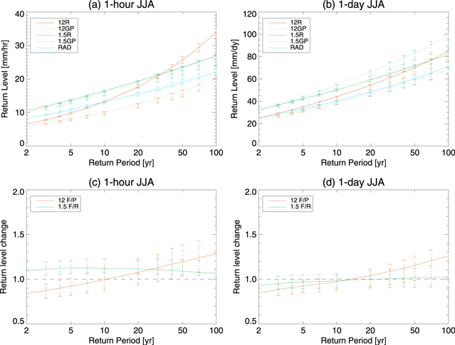
Figure 2. Upper panels: the southern UK spatial median return levels for 1 h ( ; left) and 1 day (
 ; right) precipitation; red for the 12 km RCM, green for the 1.5 km RCM, and blue for radar observations; solid line (—) for R simulations, and dots (⋯) for G-P simulations (see legend). The bottom panels show the change signal for the spatial median (
 ) between the G-P and G-F simulation. The year-jackknife-estimated confidence intervals are indicated by the error bars.
Download figure:
Standard image High-resolution image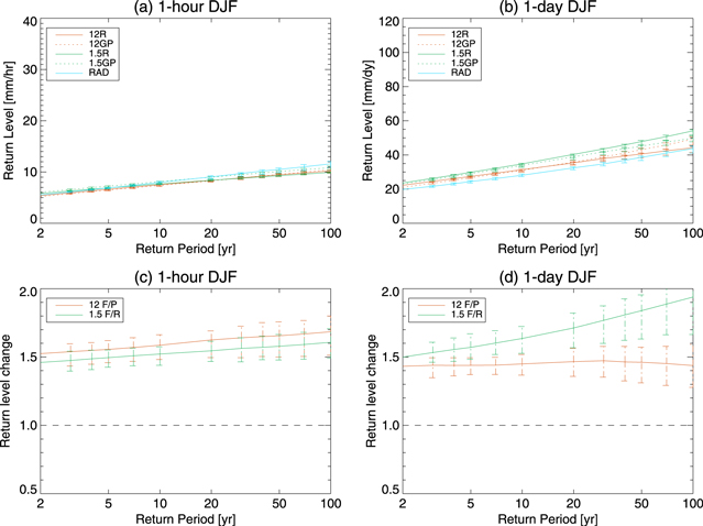
Figure 3. Same as in figure 2 except this is for DJF.
Download figure:
Standard image High-resolution image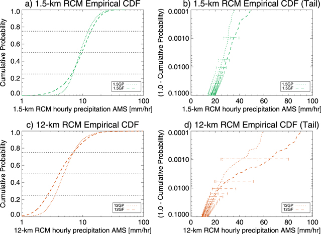
Figure 4. The cumulative distributions (full range in the left and tail in the right) of the spatially-pooled 1 h JJA maxima. The upper and lower panels are for 1.5 and 12 km RCMs respectively. The present-climate and future-climate simulations are indicated by dots (⋯) and dashes (—-) respectively. Year bootstrapping (1000 times) is used to estimate the 95% confidence intervals for the tail quantiles.
Download figure:
Standard image High-resolution imageAs in previous studies, we focus only on the summer (June–July–August; JJA) and winter (December–January–February; DJF) seasons. This gives us a better separation between localized convective precipitation and larger-scale precipitation that is associated with mid-latitude cyclones.
A related study ([3]) examines the changes in hourly precipitation characteristics (such as intensity-duration characteristics). The discussion here focuses specifically on the extreme events and EVT measures. It is important to highlight that changes in  wet-period precipitation intensities do not necessary give the same change as n-year return levels as the latter reflect changes in both the intensity and frequency of precipitation. If there are large changes in the frequency of precipitation, return level changes will be different from intensity changes. This explains the differences between results presented here and in K14.
4. Results
Figures 2 and 3 show the return levels and the projected climate change signal for JJA and DJF respectively. For JJA, the 1.5 km (12 km) RCM G-P return levels below 10 years are higher (lower) than the radar estimates. This is caused by excessive vertical velocities in the 1.5 km RCM and overly-frequent light precipitation in the 12 km RCM [2]. The 1.5 km G-F simulations show a  increase in the
  threshold (not shown) as consistent with the intensity increases in K14. However, there is a large (
 ; not shown) decrease in event frequency in both 12 km and 1.5 km RCM. These changes in event frequency are tied to changes in the length of dry periods, and they are important there as they moderate the return level changes.
The 1.5 km RCM projects JJA hourly-precipitation return levels to increase by about 10% across a wide range of return periods (figure 2(c)). The 12 km RCM projects increases in the longer ( ) return periods and decreases for shorter return periods. However, the 12 km RCM JJA projections at longer return periods have much wider CIs than the 1.5 km RCM, and overlap with the 1.5 km RCM projections; this indicates interannual variability of extremes is playing a large role in 12 km RCM projections, which are less robust than the 1.5 km RCM projections. For
  return periods, the 12 km reanalysis simulationʼs 1 h precipitation return levels exceed the 1.5 km return levels. For one day precipitation extremes, the 1 km RCM projects minimal changes for JJA, but the 12 km RCM gives the same decreases in shorter return periods and increases in longer return periods as for one hour precipitation extremes.
The large increases in long JJA return periods by the 12 km RCM are caused by sudden increases of precipitation intensity above 20  . Shown in figure 4 is the empirical distribution of the spatially-pooled summertime maxima of 1 h precipitation. The summertime maxima are taken at each land grid point, and are pooled together to form a common pool for the visualisation of the empirical distribution. Uncertainties are estimated by year-block bootstrap resampling.
For data samples below 10  , the 1.5 km RCM simulations clearly show higher intensities than the 12 km RCM simulations. However, both the present- and future-climate 12 km 1 h intensities increase rapidly above ≈20
  (right panels, figure 4). It is evident that these non-robust higher 12 km RCM intensities contribute to positive future changes for the one hour precipitation intensities. The increase appears at the very tail of summertime maxima for both 12 km simulations, and is only detectable at the tail of the empirical distribution. The increase suggests that some of these higher maxima may not follow the same probability distribution as the lower maxima. We have the least confidence in the highest intensities because sub-grid convection schemes are not designed to represent vigorous convection when the size of the convection becomes comparable with the model horizontal grid size [5, 8, 31]. To add to the lower confidence, the surge is not robust to year-to-year variability—indicating the hit-or-miss nature of these events. Yet the increase appears to play a role in the 12 km RCM projections. In general, we have low physical and statistical confidence in the actual 12 km RCM data that give the change signal for longer return periods. This is unlike the 1.5 km RCM JJA projections, which appear more robust and consistent.
Present and future DJF one hour return levels (figure 3) are generally lower than for JJA, especially at the longer ( ) return periods. The most important difference between the JJA and DJF projections are that the DJF projected changes are much larger. A 40–60% and 40–90% return level increase is projected by both the 12 km and 1.5 km RCM for 1 h and 1 day precipitation extremes respectively. The DJF projections are so large that they are well beyond uncertainties caused by year-to-year sampling issues. Interestingly, the increases in DJF 1 day extremes are higher in the 1.5 km RCM compared to the 12 km RCM (figure 3(d)). That is despite both simulations showing comparable 1 h return level projections. Overall, the projections are suggesting a stronger role of winter extremes in the future on the daily timescale.
In figure 1, we show maps of the 10 years return level projections for JJA 1 h and DJF 1 day extremes. The projections for JJA 1 h extremes are spatially 'noisy' for both the 12 km and 1.5 km RCM with no clear spatial patterns, but the 1.5 km RCM projections have more grid points with positive change (hence the more robust estimates in figure 2). The local 'noisiness' of the JJA projections indicates that grid-box-scale projections are not robust nor informative, and the JJA change signal is only clear as a regional estimate.
Positive changes occur nearly everywhere for DJF 1 day projections. There are signs for larger positive changes over the Welsh orography. That is coincident with the largest DJF 1 day events for both models, which indicates that these events are associated with orographic precipitation enhancement (not shown). The Welsh enhancements are larger for the 1.5 km RCM, so the DJF differences may be linked to the different orographic representation between the two RCMs, which may affect multi-hour accumulations more than 1 h accumulations. We do note that not all orographic regions see higher projections; the 12 km RCMʼs projections over Dartmoor and the Pennines are weaker. The intensification of DJF extremes has been found by lower-resolution RCMs; the difficulty has always been in obtaining robust JJA change signals [1, 15].
The JJA increase in 1.5 km RCM return levels ( ) are more moderate than the change in the heavy precipitation intensity (
 ) [3]. The number of selected extreme events depends on the frequency of precipitation. The above is illustrated in figure 5 where we visualize the stochastic matrix of the state changes between 'dry' (state 1: P
  ) and 'wet' (state 2: P
  ) hours. The probabilities of triggering precipitation (1-to-2) and remaining in a dry state (1-to-1) are essentially RCM-independent under the same lateral boundary conditions (LBCs). The 1-to-1 and 1-to-2 probabilities only change when the LBCs are changed. As the probabilities of moving from a dry to a wet state are decreased in the future simulations, the future simulations have longer dry spells. While precipitation duration (the 2-to-2 and 2-to-1 probabilities) is thought to be tied to model physics6
, the precipitation triggers are much more driven by large-scale conditions. It is important to highlight that this result is produced by two different RCMs with large differences in precipitation intensities.
) hours. The probabilities of triggering precipitation (1-to-2) and remaining in a dry state (1-to-1) are essentially RCM-independent under the same lateral boundary conditions (LBCs). The 1-to-1 and 1-to-2 probabilities only change when the LBCs are changed. As the probabilities of moving from a dry to a wet state are decreased in the future simulations, the future simulations have longer dry spells. While precipitation duration (the 2-to-2 and 2-to-1 probabilities) is thought to be tied to model physics6
, the precipitation triggers are much more driven by large-scale conditions. It is important to highlight that this result is produced by two different RCMs with large differences in precipitation intensities.
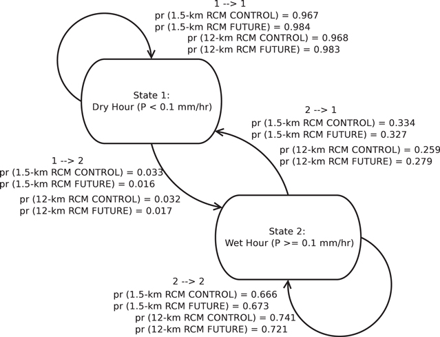
Figure 5. The graphical representation of the RCM-simulated JJA Markov stochastic matrix between 'dry' (state 1) and 'wet' hours (state 2). 'Wet' is defined to have hourly precipitation in excess of 0.1  .
.
Download figure:
Standard image High-resolution imageThis above result has important implications for drought projections: the 12 km RCM appears to be sufficient for projecting changes in dry spell length, providing changes in the large-scale conditions inherited from the driving GCM are reliable. In other words, reduction of GCM circulation biases is key for useful drought projections. It also illustrates that the problem with the 12 km RCM return level projections is tied to poor simulations of precipitation intensity, and not so much with the LBCs.
5. Discussion and conclusions
It is clear that our extreme projections are highly sensitive to model physics, but we are more confident in the physical realism of the 1.5 km RCM extremes. The 1.5 km model projects a uniform increase (≈10 %) in the spatial median for JJA hourly return levels across a range of return periods. We have low physical confidence in the 12 km RCM JJA return level projections, which are different from the 1.5 km RCM projections although not significantly so for long return periods. The JJA uncertainty estimates have become narrower with the use of the 1.5 km RCM, which by itself is a substantial improvement.
Results here are for a single model. The high computational cost poses as a significant limitation to the length of our simulations. Long and multi-ensemble simulations would be necessary to give better quantification to inter-annual variability. In the future, we hope there will be more convective permitting RCM simulations, so that model uncertainty can be better quantified. We have also not tested the sensitivity of our projections to different driving LBCs. Circulation differences (like the latitudinal position of the Atlantic Jet Stream or the frequency of blocking events) are likely to have large impacts on both JJA and DJF projections.
The intensification of winter (DJF) extreme precipitation has been projected by a number of studies with coarser resolution RCMs (see section 1). For the UK, our projections with a convective-permitting RCM are consistent with these coarser-resolution RCM projections. It is summer when the projections diverge most strongly. We do wish to note that the convective-permitting RCM does yield a higher DJF projection than the 12 km RCM for daily extremes, and this may be related to the different representations of the orography. This situation is different for summer, when we have physical reasons (i.e. the convective parameterisation) to be suspicious of the 12 km large intensity precipitation events.
The probability distribution discontinuity at ≈20  in the 12 km RCM looks unusual. Physically non-plausible higher precipitation intensities in convection parameterised models are well documented in the literature [31]. In previous work [5], we show that such high intensities are linked, at least in some cases, to grid point storms in the 12 km RCM. These occur where there is grid point saturation; assumptions of the convective parameterisation breaks down as convective cells approach the size of the model grid scale. Such grid point storms are expected to be a particular problem for model resolutions in the 'gray zone' (such as the 12 km RCM), and may be expected to occur less often in coarser resolution models. Indeed, we find that a 50 km-resolution RCM [7] does not show a marked discontinuity at high values (not shown). However, we note that the other deficiencies in hourly precipitation (such as its diurnal cycle and duration) are seen for all models with convection parameterisation, and such deficiencies do not improve at coarser resolutions.
JJA extremes are associated with convective events. As convective events are highly localised, return level changes are noisy spatially. Computationally-expensive longer model integrations are necessary to reduce the horizontal scale that confident statements about extreme changes can be made.
While our results highlight the potential value of explicit convection models for the simulation of heavy precipitation events in present and future climate, the computational costs are expensive, and the enhanced value is largely limited to summer only. While computational power may increase in future, the use of convective parameterisation is likely to be unavoidable in the near future. As previously found [7], the 12 km RCM does provide good simulations for certain measures. The key message here is that modellers should be aware of the limitations that are posed by the model physics, and be wary of how these limitations can affect the reliability of model results.
Despite different JJA return level projections, both the 12 km and 1.5 km simulations agree on the decrease of extreme event and precipitation frequency in the future. This suggests that conditions favourable (or unfavourable) to precipitation are controlled at the larger scale which both RCM simulations share. Even the 1.5 km RCM projects heavy precipitation to intensify, it does not necessary lead to same increase in return levels as wet days and hours become rarer. Probability of triggering precipitation is independent of model (figure 5). As far as our simulations are concerned, the model differences appear to impact mostly on precipitation intensities and duration [3]. It is essential to remember that there are two issues here: large-scale circulation and humidity changes that are controlled by the LBCs, and precipitation intensity changes that are sensitive to regional model physics. The LBCs do matter for extreme projections; that is because the LBCs control the probability of extreme events. For our simulations, it is up to the individual model physics to produce the right summer (convective) precipitation intensities. It is the latter that distinguishes the two RCMs; without realistic precipitation physics, the hope of simulating realistic precipitation extremes is remote.
While the two RCMs disagree on extreme event intensification, both suggest longer dry periods in the future JJAs. It has been postulated that precipitation intensity should intensify in a warmer climate as atmospheric humidity scales with temperature [32], and indeed there are intensifications of simulated precipitation intensities. The 1.5 km RCM projection can be succinctly summarised as containing longer dry spells but with more intense extremes. This is 'double bad news' for stakeholders—an increased risk of flash flooding and meteorological drought7 . Bursts of intense precipitation increases surface run-off as recharge of subsurface water becomes limited by surface infiltration rate, hence there is a more limited levitation of hydrological drought conditions. It has been argued that the short-duration extreme events would intensify more than the daily averages due to dynamical feedbacks [33, 34]. We shall explore this issue in a future paper.
Acknowledgments
This research is part of the CONVEX (grant: NE/I006680/1) and INTENSE (grant: ERC-2013-CoG) projects. We would like to thank Dr CA Ferro of the University of Exeter for his input to our work. CONVEX is supported by the United Kingdom National Environmental Research Council and the UKMO. INTENSE is supported by the European Research Council. We gratefully acknowledge funding from the Joint Department of Energy and Climate Change and Department for Environment Food and Rural Affairs Met Office Hadley Centre Climate Programme (GA01101). Large portions of the analysis have been carried out with the free-and-open-source software R.
Footnotes
- 5
'Gray-zone' refers to the model resolutions that atmospheric moist convection becomes partially resolvable—usually on the order of
 [8], and for which convective parameterisation assumptions become invalid.
 - 6
Precipitation duration differences of the two models have been previously demonstrated [2].
- 7
Meteorological droughts are shortfalls of precipitation; and this is contrary of hydrological droughts which are shortfalls of subsurface water supply.
