
Abstract
Worldwide, lack of data on stream temperature has motivated the use of regression-based statistical models to predict stream temperatures based on more widely available data on air temperatures. Such models have been widely applied to project responses of stream temperatures under climate change, but the performance of these models has not been fully evaluated. To address this knowledge gap, we examined the performance of two widely used linear and nonlinear regression models that predict stream temperatures based on air temperatures. We evaluated model performance and temporal stability of model parameters in a suite of regulated and unregulated streams with 11–44 years of stream temperature data. Although such models may have validity when predicting stream temperatures within the span of time that corresponds to the data used to develop them, model predictions did not transfer well to other time periods. Validation of model predictions of most recent stream temperatures, based on air temperature–stream temperature relationships from previous time periods often showed poor performance when compared with observed stream temperatures. Overall, model predictions were less robust in regulated streams and they frequently failed in detecting the coldest and warmest temperatures within all sites. In many cases, the magnitude of errors in these predictions falls within a range that equals or exceeds the magnitude of future projections of climate-related changes in stream temperatures reported for the region we studied (between 0.5 and 3.0 °C by 2080). The limited ability of regression-based statistical models to accurately project stream temperatures over time likely stems from the fact that underlying processes at play, namely the heat budgets of air and water, are distinctive in each medium and vary among localities and through time.
Export citation and abstract BibTeX RIS

Content from this work may be used under the terms of the Creative Commons Attribution 3.0 licence. Any further distribution of this work must maintain attribution to the author(s) and the title of the work, journal citation and DOI.
Introduction
Lack of available long-term data on stream temperatures has been recognized as a major limitation for understanding thermal regimes of riverine ecosystems (Webb et al 2008, Arismendi et al 2012). This has motivated the application of a host of models that use more widely available alternative surrogates for predicting stream temperature (e.g., Eaton and Scheller 1996, Erickson and Stefan 2000, Van Vliet et al 2011, Hill et al 2013). Regression based statistical models that use air temperature as the predictor of stream temperatures are particularly popular (Kothandaraman 1972, Mohseni et al 1998, Erickson and Stefan 2000, Bogan et al 2003). These models have been used extensively in the United States for projecting future stream temperatures, with estimated increases ranging between 1° and 9 °C by the year 2050 (e.g., Cooter and Cooter 1990, Stefan and Sinokrot 1993, Mohseni et al 2003, Mantua et al 2010). Such changes in stream temperature would have dramatic implications for stream ecosystems (Magnuson et al 1979, Vannote and Sweeney 1980, McCullough et al 2009), particularly cold-water species (Heino et al 2009, Beechie et al 2012).
Although, stream temperatures based on surrogates such as air temperature can be readily modeled, the actual processes governing the heat budget of streams are quite complex and include a myriad of climatic, non-climatic, and human factors and their interactions (Johnson 2003, Webb et al 2008, Hester and Doyle 2011, Arismendi et al 2012). Relationships between air and stream temperatures are driven mostly by the fact that both are heated by net solar radiation, with other processes linking air and stream temperatures are relatively minor (Sinokrot and Stefan 1993, Bogan et al 2003, Johnson 2004, Webb et al 2008, Benyahya et al 2010, Diabat et al 2012). With respect to the heat flux in streams changing climates, water uses, and land cover, many processes that modify the influence of solar radiation on stream temperatures have potential to change, including streamflow regimes (Jefferson 2011, Arismendi et al 2013, Safeeq et al 2013), the type and distribution of riparian vegetation (Capon et al 2013), groundwater (Taylor et al 2013), as well as solar radiation itself (Wild 2012). Because the heat budgets of air and streams differ, there is no reason to expect that contemporary statistical correlations will remain stationary over time. The contribution of different processes governing heat budgets in streams will change substantially as the effects of climate-related and other changes are realized (Cassie et al 2001). Accordingly, the widespread practice of applying relatively short-term air-stream temperature associations to project long-term future stream temperatures merits further scrutiny.
Here, using existing historical datasets for stream and air temperatures from natural and highly human-influenced watersheds, we investigated the long-term performance of widely used linear and nonlinear regression models for predicting stream temperatures. Our first objective was to evaluate the temporal variability of parameters that comprise these air-stream temperature models over sequential 5-year periods and among sites. The second objective was to evaluate potential uncertainties of these models for projections of stream temperatures over longer time periods such as in the case of climate change related questions. As an illustrative exercise, we validated these models by comparing most recent observed stream temperature values (2005–2009) to predictions from models that were parameterized with data from previous 5-year periods. In addition, we evaluated the performance of these models in predicting and detecting extreme cold and warm stream temperature conditions (defined herein as the coldest and warmest temperatures within the period of data collection). We hypothesized that if air plays an important role driving the magnitude of temperature in streams, there should be a relatively stationary association or consistency in parameters that define associations between air and stream temperatures across time periods. Overall, our evaluation of the performance of these models over time allowed us to evaluate the efficacy of using purely climate factors, such as air temperature, to project future effects of climate change and other human-related influences on stream temperatures.
Methods
Study sites and time series
We selected 25 sites (supplementary table 1) with long-term, year-round daily mean stream temperature data in the western (California, Oregon, Idaho, Washington, and Alaska) United States. These sites represent a broad diversity of hydroclimatic settings with varying degrees of flow regulation, and are thus suitable for addressing our fundamental objectives in this work. The numbers and locations of our study sites are restricted to available datasets that were appropriate to examine the long-term performance of these empirical models. In their extensive review of the available literature about stream temperature Webb et al (2008) highlight the scarcity of long-term stream temperature data available around the world. Fortunately in western North America there are some sites with long-term data that have not been affected by major changes in water and land use over time, allowing researchers to examine the effects of purely climatic drivers on stream temperature (e.g., Arismendi et al 2012). We selected sites with more than 11 years of data; the mean length of the available time series was 25 years and the longest period considered was 1965–2009. The number of sites with stream temperature data in any given year ranged from 1 to 25, with the greatest number of sites having data from 1999–2009. Because some sites were affected by dams, water diversion, and more intense land-use changes, we separated the 25 sites into minimally (hereafter unregulated sites; n = 11) and highly (hereafter regulated sites; n = 14) human-influenced watershed groups (based on Falcone et al 2010; supplementary table 1).
Surface air temperature data were not available for the full study period from each site. Many studies using the methods evaluated herein faced similar challenges and used point data from sites that were variably distant from where stream temperatures were recorded. We were most interested in broad-scale relationships and thus evaluated air temperatures that were averaged over the catchment for each stream rather than a point measurement as near as possible to the stream temperature site. Our choice was based on the typically broad scales for which the method we evaluated is applied (e.g., Mantua et al 2010). We used existing gridded temperature data that represent approximately 20 000 National Climatic Data Center (NCDC) Coop stations across the contiguous United States (Livneh et al 2013). We calculated air temperature for our sites, except those in Alaska, as the arithmetic mean of 1/16-degree resolution (approximately 30 km2) gridded daily minimum and maximum surface temperature data. For each stream temperature site, the air temperature data from nearest grid cell was selected. In Alaska, we obtained air temperature data from the nearest NCDC Coop station. We acknowledge air temperatures that provide input or validation for gridded meteorological data may be underrepresented in complex mountainous terrain (Daly et al 2008).
Previous research has shown strong correlations between air and stream temperature at various time scales (Kothandaraman 1972, Mohseni et al 1998, Erickson and Stefan 2000, Bogan et al 2003). Specifically, correlations are typically weak at a daily time scale (e.g., Erickson and Stefan 2000) whereas a coarser time scale (e.g., monthly) can lead to the compression of variability and thus, a loss of potentially relevant information. Accordingly, weekly time scales have been widely adopted for regulatory purposes (Groom et al 2011) and biological relevance (Mohseni et al 2003, Mantua et al 2010). Thus, to be most comparable to published models of stream-air relationships, we calculated mean weekly air and water temperatures from the daily values at each of the 25 sites.
Correlation models and data analyses
To test the predictive power of air-stream temperature relationships using long-term historical data, we performed a linear regression analysis between stream and air temperatures (Webb and Nobilis 1997, Erickson and Stefan 2000). Linear regression was applied as:
where Ts (t) and Ta (t) represented weekly mean stream and air temperature (°C) respectively at a specified time t, A the y-intercept (°C) of the regression line, and B the slope (°C/°C) of the line.
We also used the nonlinear regression model for mean stream temperatures proposed by Mohseni et al (1998):
where Ts was the estimated weekly mean stream temperature, μ the estimated minimum stream temperature, α was the estimated maximum stream temperature, γ was a measure of the steepest slope of the function, β was the air temperature at the inflection point, and Ta was the observed weekly mean air temperature. We estimated the model parameters α, β, γ, and μ, using iterative least squares estimation in MATLAB (MathWorks 2011). To ensure a positive value of stream temperature (these rivers do not freeze), we assigned zero as the lower limit of μ.
Several previous studies have characterized the air and water temperature relationship using data from a 3-year timeframe (Eaton and Scheller 1996, Mohseni et al 1998). However, others have suggested that a 3-year period was insufficient to describe the relationship between air and stream temperature (Erickson et al 1998). Therefore, for each model parameterization, we used concurrent mean weekly water and air temperature data for a five year period (260 weeks or data points). The start and end of the each 5-year period was consistent across sites. We did not perform the regression analysis if the air or water temperature data was missing for more than four weeks in each 5-year period. We performed both linear and nonlinear regression analysis using data from each 5-year period over the length of each available time series.
We evaluated the accuracy of predicted stream temperatures from the two regression models using the root mean squared error (RMSE) statistic. The RMSE represented the standard deviation (SD) of the predicted stream temperatures about the observed values and was on the same scale as the data (°C). The magnitude of each RMSE value indicated that approximately 68% of the predicted stream temperature values were within one SD of the observed values, 95% were within two SD, and 99% were within three SD. An optimal value of RMSE is zero. We also used Nash–Sutcliffe efficiency (NSE; Nash and Sutcliffe 1970), which measures the relative magnitude of the residual variance of the modeled stream temperatures to the variance of the observed stream temperatures. The NSE ranges from −∞ to 1 where NSE = 1 corresponds to a perfect match of modeled to the observed temperature.
We examined the association between both the magnitude and variability of the RMSE and NSE statistics and potentially relevant watershed characteristics (i.e., latitude, longitude, elevation, drainage area, slope, aspect northness, mean annual discharge, baseflow index, % of riparian forest; Falcone et al 2010) using the Spearman's rank order correlation analysis. We performed these statistical analyses using the software R ver. 2.11.1 (R Development Core Team 2005).
To illustrate potential uncertainties in using this correlation approach in long-term future projections of stream temperatures we applied parameters that defined the linear and nonlinear models for each 5-year time period and validated the performance of each model for the most recent period 2005–2009. We then compared the observed stream temperature data for this period (2005–2009) to that from the model predictions based on past time periods using the RMSE statistic and examined the residuals (predicted—observed). Because we were focused on the long-term variability of the parameters across each 5-year time period, we applied this analysis to the two longest time series available at both human-regulated (Martis Creek, CA; Clearwater River, ID) and unregulated sites (Fir Creek, OR; Elk Creek, OR). We repeated this analysis to illustrate the uncertainties in long-term future projections of extreme cold and warm weekly stream temperature conditions using the RMSE statistic. The extreme cold and warm conditions (within the period of record) were approximated as temperature departure of one SD below and above the mean, respectively. In addition, we tested the ability of these models to detect extreme stream temperature events (i.e., weeks) that exceeded (mean + 1 SD) or were below (mean − 1 SD) mean observed conditions over each 5-year time periods using a success index (SI; van Aalst and de Leeuw 1997, Singh et al 2011):
where A represented the number of correctly estimated events exceeding (or that were below) mean conditions, M was all observed events that exceeded (or were below) mean conditions, N was the total number of events, and F represented all estimated events considered that exceeded (or were below) mean conditions. The SI estimates both the number of events exceeding (or above) and non-exceeding (or below) mean conditions and ranges between −100 to 100 with a best value of 100.
Results
Overall performance of the models and variability of parameters across time periods
The mean RMSE of the linear model in predicting stream temperature during the different 5-year time periods were similar than the nonlinear model in all sites (table 1). For the regulated sites, the RMSE using linear models ranged between 0.8 °C and 2.1 °C (mean of 1.4 °C) and using nonlinear models ranged between 0.8 °C and 1.9 °C (mean of 1.3 °C). For the unregulated sites, the RMSE ranged between 0.8 °C and 1.7 °C (mean of 1.2 °C) for the linear models and between 0.7 °C and 1.6 °C (mean of 1.1 °C) for the nonlinear models. The highest variability for the RMSE occurred for the nonlinear model in the regulated S2 (0.63 °C). The linear model showed higher variability (SD) for the RMSE than the nonlinear model in 57% of the regulated and 55% of the unregulated sites. Further, the mean NSE of the two models for all sites showed similar values (0.86 and 0.87 for the linear and nonlinear model respectively). However, the mean NSE of the linear model in predicting stream temperature during the different 5-year time periods was lower than the nonlinear model in eight of the fourteen regulated sites and in all of the unregulated sites. The highest variability for the NSE occurred for the linear model in the regulated S9. Overall, the linear model showed higher variability (SD) for the NSE than the nonlinear model in 71% of the regulated and 45% of the unregulated sites.
Table 1. Root mean square error (RMSE) and Nash–Sutcliffe efficiency (NSE) values for the two correlation models (l = linear; nl = nonlinear) in regulated (n = 14) and unregulated (n = 11) streams. Values correspond to mean and SD estimated for sequential or multiple 5-year periods.
| Site type | Site ID | Mean RMSE_l | SD RMSE_l | Mean RMSE_nl | SD RMSE_nl | Mean NSE_l | SD NSE_l | Mean NSE_nl | SD NSE_nl |
|---|---|---|---|---|---|---|---|---|---|
| Regulated | S1 | 2.12 | 0.21 | 1.87 | 0.21 | 0.87 | 0.03 | 0.90 | 0.03 |
| S2 | 1.48 | 0.63 | 1.43 | 0.64 | 0.93 | 0.06 | 0.94 | 0.06 | |
| S3 | 1.27 | 0.08 | 1.20 | 0.08 | 0.96 | 0.01 | 0.96 | 0.01 | |
| S4 | 1.27 | 0.02 | 1.23 | 0.02 | 0.95 | 0.00 | 0.95 | 0.00 | |
| S5 | 1.28 | 0.29 | 1.27 | 0.29 | 0.82 | 0.05 | 0.82 | 0.05 | |
| S6 | 0.92 | 0.12 | 0.87 | 0.11 | 0.94 | 0.02 | 0.94 | 0.01 | |
| S9 | 1.63 | 0.18 | 1.58 | 0.19 | 0.69 | 0.09 | 0.71 | 0.08 | |
| S10 | 1.20 | 0.10 | 1.15 | 0.12 | 0.83 | 0.04 | 0.85 | 0.05 | |
| S11 | 1.36 | 0.14 | 1.34 | 0.14 | 0.72 | 0.05 | 0.73 | 0.05 | |
| S12 | 2.09 | 0.37 | 1.94 | 0.35 | 0.81 | 0.03 | 0.84 | 0.03 | |
| S13 | 1.09 | 0.13 | 0.98 | 0.12 | 0.91 | 0.02 | 0.93 | 0.02 | |
| S15 | 0.84 | 0.05 | 0.80 | 0.06 | 0.92 | 0.01 | 0.92 | 0.01 | |
| S17 | 1.60 | 0.08 | 1.48 | 0.04 | 0.92 | 0.02 | 0.93 | 0.01 | |
| S18 | 1.29 | 0.14 | 1.27 | 0.15 | 0.78 | 0.03 | 0.78 | 0.03 | |
| Unregulated | S7 | 0.83 | 0.08 | 0.78 | 0.07 | 0.90 | 0.02 | 0.91 | 0.01 |
| S8 | 1.49 | 0.06 | 1.38 | 0.09 | 0.85 | 0.01 | 0.87 | 0.02 | |
| S14 | 1.09 | 0.11 | 1.01 | 0.10 | 0.87 | 0.02 | 0.89 | 0.02 | |
| S16 | 1.09 | 0.09 | 1.02 | 0.09 | 0.91 | 0.01 | 0.92 | 0.01 | |
| S19 | 1.71 | 0.08 | 1.58 | 0.12 | 0.94 | 0.00 | 0.95 | 0.01 | |
| S20 | 1.09 | 0.09 | 0.72 | 0.07 | 0.85 | 0.01 | 0.94 | 0.02 | |
| S21 | 1.25 | 0.11 | 1.12 | 0.10 | 0.78 | 0.06 | 0.82 | 0.05 | |
| S22 | 1.02 | 0.05 | 0.78 | 0.01 | 0.89 | 0.00 | 0.94 | 0.00 | |
| S23 | 1.39 | 0.13 | 1.32 | 0.13 | 0.84 | 0.03 | 0.86 | 0.02 | |
| S24 | 1.43 | 0.16 | 1.37 | 0.17 | 0.77 | 0.04 | 0.79 | 0.04 | |
| S25 | 1.24 | 0.12 | 1.20 | 0.14 | 0.78 | 0.03 | 0.80 | 0.03 |
The magnitude of the slope and intercept for the linear model (figure 1) was highly variable among sites and across time periods (slope: 0.32–1.01; intercept: 0.37–6.87 °C). The widest range of slope magnitude and variability over time periods occurred in regulated sites compared to unregulated sites (0.01–0.11 SD versus 0.004–0.04 SD). For example, the slope of the linear model in S12 (regulated) decreased by 200% while the intercept increased by 170% over time. The variability of the intercept values for the linear model within sites over time periods was relatively similar between regulated (0.07–0.76 °C SD) and unregulated sites (0.01–0.60 °C SD), but some sites showed high variability (e.g., regulated S1, S12 and unregulated S24, S25). Within sites, the values of slope and intercept of the linear models originating from the most recent two time periods (2000–2004 and 2005–2009) were not necessary nearest neighbors. This was illustrated for the intercept in S3, S5 and S7 (regulated) and for both intercept and slope for S19 (unregulated).

Figure 1. Temporal variability for the parameters that define (a) the linear (intercept and slope) and (b) nonlinear (α, β, γ, and μ) correlation models between air and water temperature in regulated (left panel) and unregulated (right panel) streams at different time periods. Each symbol represents a 5-year time period. Open squares represent the last two periods 2000–2004 and 2005–2009.
Download figure:
Standard image High-resolution imageAs with the linear model, the variability of all parameters that defined the nonlinear model (figure 1) was high among sites and across time periods (α: 8.0–32.6 °C, β: 5.0–19.1 °C, γ: 0.12–0.43 1/C°, and μ: 0.0–9.2 °C). In particular, within sites the parameters that described the extreme minimum (μ) and maximum (α) weekly temperatures showed a wide range of values across time periods, but higher variability occurred in regulated sites (μ: 0.00–3.45 °C SD; α: 0.25–6.83 °C SD) compared to unregulated sites (μ: 0.0–1.23 °C SD; α: 0.11–2.94 °C SD). Within sites and similar to the linear model, the values of the parameters that defined the nonlinear model originating from the two most recent time periods were not necessary nearest neighbors (e.g., for α see regulated S3, S13 and unregulated S19, S23; for μ see regulated S5, S9, S17 and unregulated S14, S23, S24).
There were statistically significant associations between the performance of the linear and nonlinear models and several watershed characteristics (table 2). In particular, the magnitude and variability of the RMSE for the two models increased, suggesting lower accuracy when the baseflow index increased. Similarly, for the linear model, when the baseflow index increased the magnitude of the NSE decreased suggesting lower performance, and the variability increased for both linear and nonlinear models. The performance of the two models also showed a significant decrease at higher elevations and lower latitudes.
Table 2. Spearman rank correlation between both mean and standard deviation (SD) of root mean square error (RMSE) and Nash–Sutcliffe efficiency (NSE) statistics for the two model (l = linear; nl = nonlinear) and selected watershed characteristics.* Denotes significance at P < 0.1, ** P < 0.05 and *** P < 0.01.
| Watershed characteristicsa | RMSE_l | SD RMSE_l | RMSE_nl | SD RMSE_nl | NSE_l | SD NSE_l | NSE_nl | SD NSE_nl | n |
|---|---|---|---|---|---|---|---|---|---|
| Latitude | −0.38 | −0.22 | −0.44 | −0.34 | −0.35 | 0.04 | −0.23 | 0.08 | 25 |
| P-value | 0.06* | 0.29 | 0.02** | 0.09* | 0.08* | 0.83 | 0.26 | 0.70 | |
| Longitude | 0.25 | 0.13 | 0.14 | 0.24 | 0.02 | 0.26 | −0.07 | 0.22 | 25 |
| P-value | 0.20 | 0.66 | 0.58 | 0.23 | 0.92 | 0.21 | 0.75 | 0.29 | |
| Elevation | 0.44 | 0.26 | 0.42 | 0.40 | −0.38 | 0.15 | −0.43 | 0.19 | 25 |
| P-value | 0.02** | 0.20 | 0.03** | 0.04** | 0.06* | 0.47 | 0.03** | 0.35 | |
| Drainage area | 0.12 | 0.09 | 0.11 | 0.08 | 0.20 | −0.13 | 0.24 | −0.12 | 23 |
| P-value | 0.60 | 0.69 | 0.61 | 0.71 | 0.36 | 0.55 | 0.26 | 0.57 | |
| Slope | 0.04 | −0.05 | 0.07 | 0.06 | −0.43 | 0.29 | −0.43 | 0.38 | 14 |
| P-value | 0.87 | 0.86 | 0.80 | 0.83 | 0.11 | 0.29 | 0.11 | 0.16 | |
| Aspect northness | 0.27 | 0.42 | 0.23 | 0.27 | −0.13 | 0.31 | −0.09 | 0.25 | 14 |
| P-value | 0.34 | 0.13 | 0.42 | 0.34 | 0.66 | 0.27 | 0.75 | 0.38 | |
| Mean annual discharge | −0.02 | 0.14 | 0.06 | 0.13 | 0.01 | 0.03 | 0.01 | 0.00 | 24 |
| P-value | 0.91 | 0.51 | 0.76 | 0.55 | 0.96 | 0.87 | 0.97 | 0.99 | |
| Base flow index | 0.49 | 0.61 | 0.49 | 0.69 | −0.45 | 0.44 | −0.39 | 0.46 | 14 |
| P-value | 0.07* | 0.01** | 0.07* | <0.001*** | 0.09* | 0.09* | 0.16 | 0.09* | |
| % Of riparian forest (100 m buffer) | −0.46 | −0.13 | −0.45 | −0.26 | 0.04 | −0.21 | 0.01 | −0.16 | 14 |
| P-value | 0.12 | 0.66 | 0.11 | 0.36 | 0.88 | 0.46 | 0.98 | 0.58 |
aFalcone et al (2010).
Predictive curves from parameter values across time periods
Predictive curves resulting from estimated parameters using different 5-year periods differed in shape across the time periods, site condition (regulated or unregulated), and if extreme cold or warm conditions were predicted (figure 2). For example, in the regulated Clearwater River (S12) with an air temperature of 30 °C, there was up to 10.6 °C for linear, and 16.4 °C for nonlinear, difference in predictions of stream temperatures across time periods. At the same site, air temperatures of −5 °C led to model output of up to 4.0 (linear) and1.6 (nonlinear) °C of difference among predicted stream temperatures. For the unregulated site at Elk Creek (S19), air temperatures of 30 °C led to 2.6 °C linear and 2.8 °C (nonlinear) difference in predicted stream temperatures across time periods, and air temperature of −5 °C resulted in up to 1.3 °C (linear) and 2.1 °C (nonlinear) of difference. For the other sites, we did not observe many differences of the predictive curves across time periods, especially for the linear model using non-extreme values of air temperature.
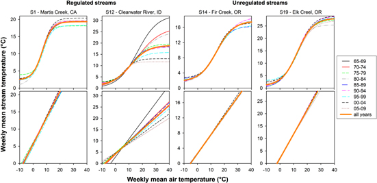
Figure 2. Illustrative examples of the weekly mean air and stream temperature predictive curves based on the nonlinear (upper panel) and linear (lower panel) models using different timeframes in two regulated and two unregulated streams. Each curve represents either a 5-year period (thin line) or all available years (bold line). Note that the shapes of predictive curves are determined by differing parameter values in the models for each time period (see figure 1).
Download figure:
Standard image High-resolution imagePredicting most recent observed stream temperatures based on past time periods
The distribution of residuals for model validation differed depending on the site, the model, the extreme cold or warm condition to be predicted, and the time period selected (figure 3, supplementary figures 1 and 2). In the regulated Clearwater River (S12), overestimation of stream temperatures was the highest during summer (figure 3; values exceed observed value for the nonlinear model by up to 14 °C) and the underestimation was the highest in January and November (values are under the observed value for the linear model by up to 12 °C). In regulated Martis Creek (S1), however, the overestimation of stream temperature was the highest during March and the underestimation was the highest in January and November, both using the linear model. In unregulated Fir Creek (S14), overestimations of stream temperature occurred during spring for both models and the underestimations were highest during summer and fall for both models. In unregulated Elk Creek (S19), there were greater number as well as higher overestimations than underestimations of stream temperature. In general, regulated sites showed higher over-and-underestimations of stream temperature than unregulated sites (supplementary figures 1 and 2).

Figure 3. Distribution of residuals in two regulated (purple symbols) and two unregulated (green symbols) streams. Each circle represents a residual from the linear (a) and nonlinear (b) model predicting weekly stream temperatures for the period 2005–2009 using parameters based on different 5-year periods. X-symbols represent observed stream temperatures for the period 2005–2009.
Download figure:
Standard image High-resolution image
For these sites with the longest available time series records, the mean performance of the linear and nonlinear models changed when we validated only the most recent (2005–2009) extreme cold and warm conditions using estimated parameters based on previous time periods (supplementary table 2). Specifically, compared to the overall perspective (table 1), the accuracy of the two models for extreme conditions was lower at Clearwater River (S12; regulated), Fir Creek (S14; unregulated), and Elk Creek (S19; unregulated), but higher at Martis Creek (S1; regulated). In addition, in accordance with the majority of our results, the two models showed a limited ability to detect observed weeks with extreme cold and warm conditions using parameters from past time periods (table 3). Specifically, the linear model showed mean values of SI between 43% and 73% per site, whereas the nonlinear model showed a mean SI between 65% and 73% per site. Only in the case of Elk Creek did the models perform relatively well, with both models having an SI above 70% for all time periods for the linear model and for six of the seven time periods for the nonlinear model.
Table 3. Success index (SI) for both linear and nonlinear models in predicting colder (mean − 1 SD) and warmer (mean + 1 SD) weekly events in two unregulated and two regulated streams using different time periods.
| Success index (SI) for 2005–2009 based on each 5-year period | |||||||||||
|---|---|---|---|---|---|---|---|---|---|---|---|
| Model | Site ID | Site | 65–69 | 70–74 | 75–79 | 80–84 | 85–89 | 90–94 | 95–99 | 00–04 | 05–09 |
| Linear | S1 | Martis Creek, CA | 53.5 | 65.5 | 56.8 | 63.0 | 54.5 | 64.2 | 63.1 | ||
| S12 | Clearwater River, ID | 47.0 | 47.0 | 42.7 | 44.3 | 48.0 | 45.8 | 46.3 | 41.1 | 31.0 | |
| S14 | Fir Creek, OR | 54.1 | 64.2 | 61.4 | 57.9 | 70.0 | 68.0 | ||||
| S19 | Elk Creek, OR | 73.5 | 72.0 | 73.8 | 74.8 | 73.5 | 73.8 | 71.5 | |||
| Nonlinear | S1 | Martis Creek, CA | 45.9 | 68.5 | 67.8 | 69.9 | 67.6 | 69.8 | 70.1 | ||
| S12 | Clearwater River, ID | 46.4 | 49.7 | 45.2 | 44.0 | 50.8 | 47.8 | 48.8 | 44.0 | 44.8 | |
| S14 | Fir Creek, OR | 64.5 | 67.0 | 63.6 | 64.7 | 62.8 | 68.6 | ||||
| S19 | Elk Creek, OR | 73.5 | 74.1 | 72.2 | 72.2 | 69.9 | 72.8 | 73.2 | |||
Discussion and conclusions
Our findings highlight several limitations that are common to linear or nonlinear regressions models used to project future stream temperatures based on air temperature. Although such models may have validity when characterizing relationships over short time frames (e.g., Eaton and Scheller 1996, Mohseni et al 1998), our results show that use of these relationships over longer time periods, as well as extrapolation of model predictions to project future stream temperatures, are unlikely to be realistic. Although we did not analyze a broad range of stream types at a continental or global extent, our analysis of stream temperatures across the western portion of North America was more than sufficient to illustrate a number of specific limitations associated with statistical projections of stream temperature based on air temperature.
Temporal variability in estimated model parameters
Parameter estimates for both linear and nonlinear models of the association between air and stream temperatures varied through time within a site. Although the purely statistical formulations of the models we evaluated here are valid, we show that transferring predictions from a model developed during one time period can lead to inaccurate prediction of stream temperature in a different time period. Accordingly, such models cannot be assumed to reliably estimate the changing associations between air and stream temperatures. Lack of temporal transferability of models is likely due to changes in the actual processes influencing heat budgets. Because these processes change over time, corresponding changes in statistical associations are also likely. Thus, we recognize the importance of changes in the multiple processes that drive heat budgets of streams over time, as well as non-stationarity of resulting statistical relationships.
Our findings show that the patterns of variability in parameter estimates are not entirely consistent among sites, highlighting the importance of local influences. This finding seems reasonable considering local heat budgets of streams are influenced by a combination of climatic and other non-climate or indirect-climate drivers (Johnson 2004, Webb et al 2008). Although we did not attempt to identify a complete suite of specific factors that could explain this differential performance, our results highlight the importance of groundwater, riparian shading, latitude, and elevation. Specifically, higher groundwater influence is associated with lower model performances suggesting a low sensitivity of stream temperature to future increases in air temperature (e.g., Bogan et al 2003, Tague et al 2007, Mayer 2012, Johnson et al 2013, Luce et al 2014). In addition, the performance of the two models appears to be poorer in watersheds located at lower latitudes and higher elevations. At lower latitudes, the longer photoperiod during fall/winter may increase the influence of solar radiation and thus decrease the relative importance of convective forces to the heat budget of streams compared to higher latitudes. At higher elevations in our region, streams are often surrounded by riparian vegetation that provides shade (Johnson 2004) and influences local microclimates, effectively buffering the effects of regional air temperatures (e.g., Benyahya et al 2010). In this region, streams at higher elevations serve as important spawning and rearing habitats for salmonid fishes, which are coldwater species that should be most sensitive to warming (Heino et al 2009, Beechie et al 2012). Most of these streams are located in headwaters where long-term records are less available (e.g., Falcone et al 2010, Arismendi et al 2012, Luce et al 2014). Because warming of high elevation headwater streams may have greater biological effects in this region, their sensitivity to contemporary and future climates warrants further consideration (e.g., Luce et al 2014), and it cannot be assumed they will warm in parallel with air temperatures (Arismendi et al 2012).
Predictive performance of models and their ability to predict recently observed temperatures based on past data
We find that air temperature is generally a poor predictor of stream temperatures when applied to data that is not used in model parameterization. For the majority of sites and time periods, we show that models developed during one five-year time frame perform poorly in predicting stream temperatures in another time frame. Both linear and nonlinear model formulations yield similar qualitative results, although in some cases nonlinear models perform more poorly than a simple linear regression. We highlight that the most recent stream temperatures considered here (2005–2009) are generally not predicted very accurately by models based on past air-stream temperature regressions. The magnitude of differences in stream temperature predictions across past time periods (over a 45-year window) falls within the range equal to or greater than future projections (by year 2080) reported for streams from this region due to climate change (between 0.5 and 3.0 °C; Mantua et al 2010, Van Vliet et al 2011, Ruesch et al 2012, Wu et al 2012).
Interestingly, while our results of NSE/RMSE would typically be considered to be very good in terms of model fit (Mohseni et al 1998), the distributions of residuals and the SI index reveal a poor performance of these models in detecting extreme events. Extreme cooler or warmer temperatures are of particular importance with respect to climate-based projections especially for sensitive species. We recognize that our detection of extreme events is dampened by our metric of weekly averages, but even at this resolution, extreme events were not well modeled and these events often have high biological significance. Similar poor performance in estimating extreme temperatures using these models has been reported elsewhere in the literature (Webb and Nobilis 1995, Mohseni et al 1998, Kvambekk and Melvold 2010, Benyahya et al 2010).
Directions in modeling and projecting future stream temperatures
Our evaluation of existing regression models to predict climate influences on stream temperatures clearly shows that other alternatives are needed. In many cases where climate effects are being projected, direct estimates of stream temperature are not used, and air temperature alone is used as a surrogate (e.g., Keleher and Rahel 1996, Rieman et al 2007, Wenger et al 2011). Although these studies are intended to explore broad-scale patterns in potential climate effects, our findings suggest that alternative approaches are needed to address questions about climate effects at finer scales. Stream temperature is a particularly challenging variable because (1) suitable long times series are often unavailable (Webb et al 2008, Arismendi et al 2012), (2) many streams have temperature regimes already impacted by other human activities (Moore et al 2005, Webb et al 2008, Hester and Doyle 2011), (3) the magnitude of projected changes is small relative to the uncertainty in our predictions (e.g., Wenger et al 2013), and (4) it is strongly responsive to very localized influences (Moore et al 2005). Yet, in many places or for thermally sensitive species, a small increase in temperature may have dramatic influences on biota due to the nonlinear effect of temperature on physiological processes. Our point in this paper is not to criticize previous attempts to model and project influences of climate on stream temperatures, but rather to highlight the need to move beyond these regression approaches and explicitly acknowledge these uncertainties in assessments of climate effects.
What are potential alternative approaches to projecting effects of changing climates on stream temperatures? Because statistical approaches cannot easily model changes in underlying processes that drive relationships, spatially explicit process-based models may provide a more realistic framework to explore alternative scenarios of the future. Based on the first law of thermodynamics (thermal energy budget) and Newton's laws of motion several models have been developed (e.g., Sinokrot and Stefan 1993, Cole and Buchak 1995, Boyd 1996, Kim and Chapra 1997, Boyd and Kasper 2003, van Beek et al 2012). These process-based approaches require intensive data and computational efforts, but allow the identification of the most important drivers in the heat budget of streams across timescales, improving the resolution and accuracy of stream temperature predictions (e.g., Sinokrot and Stefan 1993, Diabat et al 2012, van Beek et al 2012). Existing evidence shows net solar radiation to be the most important driver of temperature in streams in most cases, whereas air temperature is of secondary importance (Sinokrot and Stefan 1993, Bogan et al 2003, Johnson 2004, Benyahya et al 2010, Webb et al 2008). Temperature in small- to medium-sized streams can be mediated by shade from riparian vegetation (Johnson and Jones 2000, Johnson 2004, Bogan et al 2004, Benyahya et al 2010) and groundwater inputs (Bogan et al 2003, Tague et al 2007, Mayer 2012, Johnson et al 2013). In many cases subsurface heat exchanges and flow through substrates may also play a role (Johnson 2004, Tague et al 2007, Webb et al 2008, Mayer 2012). It is clear that heat transfer in streams is a complex process. Recent efforts have been conducted to incorporate additional non-climatic predictors in statistical models (e.g., Risley et al 2003, Van Vliet et al 2011, Ruesch et al 2012, Yearsley 2009, Yearsley 2012, Hill et al 2013, Pike et al 2013), but with even more predictors included, these statistical semi-process hybrid models cannot provide the resolution and insights offered by purely process-based models. In practice, the use of statistical semi-process hybrid models to predict stream temperatures can be broadly informative for evaluating very coarse patterns across a landscape but ultimately, evaluation of local influences and processes is needed to provide a clearer understanding of the factors that drive stream temperatures and to identify effective means of climate adaptation (e.g., Sinokrot and Stefan 1993, Diabat et al 2012, van Beek et al 2012).
In conclusion, we show that linear and nonlinear statistical models are not accurately predicting changes in stream temperatures based on relationships with air temperatures. Although the simplicity of these correlational approaches can be attractive for projecting future stream temperatures, they have poor performance due to the non-stationary relationship between air and stream temperatures over time. Collectively, we hope our findings will help scientists and resource managers improve our understanding of the strengths and limitations of existing models including (1) their ability as a tool for an effective assessment of stream vulnerability, (2) to improve decision-making about alternatives for climate change adaptation, and (3) to promote best practices for addressing climate change effects in streams ecosystems.
Acknowledgements
Brooke Penaluna and two anonymous reviewers provided comments that improved the manuscript. Part of the data was provided by the HJ Andrews Experimental Forest research program, funded by the National Science Foundation's Long-Term Ecological Research Program (DEB 08-23380), US Forest Service Pacific Northwest Research Station, and Oregon State University. Financial support for IA was partially provided by US Geological Survey, the US Forest Service Pacific Northwest Research Station and Oregon State University through joint venture agreement 10-JV-11261991-055. Use of firm or trade names is for reader information only and does not imply endorsement of any product or service by the US Government.