

Abstract
Understanding the relative contributions of individual countries to global climate change for different time periods is essential for mitigation strategies that seek to hold nations accountable for their historical emissions. Previous assessments of this kind have compared countries by their greenhouse gas emissions, but have yet to consider the full spectrum of the short-lived gases and aerosols. In this study, we use the radiative forcing of anthropogenic emissions of long-lived greenhouse gases, ozone precursors, aerosols, and from albedo changes from land cover change together with a simple climate model to evaluate country contributions to climate change. We assess the historical contribution of each country to global surface temperature change from anthropogenic forcing ( Δ Ts), future Δ Ts through year 2100 given two different emissions scenarios, and the Δ Ts that each country has committed to from past activities between 1850 and 2010 (committed Δ Ts). By including forcings in addition to the long-lived greenhouse gases the contribution of developed countries, particularly the United States, to Δ Ts from 1850 to 2010 (58%) is increased compared to an assessment of CO2-equivalent emissions for the same time period (52%). Contributions to committed Δ Ts evaluated at year 2100, dominated by long-lived greenhouse gas forcing, are more evenly split between developed and developing countries (55% and 45%, respectively). The portion of anthropogenic Δ Ts attributable to developing countries is increasing, led by emissions from China and India, and we estimate that this will surpass the contribution from developed countries around year 2030.
Export citation and abstract BibTeX RIS

Content from this work may be used under the terms of the Creative Commons Attribution 3.0 licence. Any further distribution of this work must maintain attribution to the author(s) and the title of the work, journal citation and DOI.
1. Introduction
In development of intergovernmental climate change mitigation policy, countries are typically grouped by economic status or historical contribution to greenhouse gas emissions (i.e. Kyoto Protocol; United Nations Framework Convention on Climate Change (UNFCCC)). These criteria are used to assign accountability for climate change to individual nations and determine their 'common but differentiated responsibilities' for mitigation (Wei et al 2012). Initial efforts to determine country-level commitments to climate change (e.g. den Elzen and Schaeffer 2002, Höhne and Blok 2005) based accountability on greenhouse gas emissions and have culminated in two recent studies, Höhne et al (2010), who explore uncertainties in country-level contributions, and den Elzen et al (2013) who use CO2-equivalent (CO2-eq) emissions as a metric for comparison. In addition, Wei et al (2012) showed that historical CO2 emissions from fossil fuel burning and cement production in developed countries contributed 62% of the global mean surface temperature increase from 1850 to 2005.
While for the long term cumulative CO2 emissions represent a good proxy for peak temperatures (Allen et al 2009), on shorter time scales there is disagreement whether to focus on cutting CO2 or short-lived gases (e.g. Bond and Sun 2005, Boucher and Reddy 2008, Shindell et al 2012). Matthews et al (2014) attribute historical, anthropogenic Δ Ts to individual countries by weighting emissions of both long-lived greenhouse gases and short-lived sulfate aerosols according to the timescale of their legacy in affecting global temperature. However, Matthews et al (2014) do not include the aerosol direct effects from non-sulfate aerosols, aerosol indirect effects, ozone precursor gas emissions, or land albedo changes. These forcing agents are among the most uncertain in recent assessments but as absolute magnitudes, account for over 30% of the anthropogenic radiative forcing (RF) (Myhre et al 2013).
In this study we identify the relative contributions of each country to global RF and Δ Ts from greenhouse gases, including ozone and halocarbons, aerosol direct and indirect effects, land cover change, and biogeochemical feedbacks. Fundamentally this comprehensive approach is similar to Prather et al (2009) who compute RF and Δ Ts from developed countries through the year 2002 for a similar set of forcing agents, although we extend the analysis to include future forcing from individual countries. We also calculate the Δ Ts that individual countries are committed to even if all emissions were eliminated in 2010. We examine the contribution of Annex 1 (developed) and non-Annex 1 (developing) country groups as designated by the UNFCCC, to global RF and Δ Ts from 1850 through 2010, and 1850 through 2100 for two future projections—representative concentration pathways (RCP) 4.5 and 8.5. These projections are defined by a fixed year 2100 global anthropogenic RF (relative to a preindustrial environment), e.g. RCP4.5 leads to a year 2100 RF of 4.5 Wm−2 (Moss et al 2010). The two RCPs used in this study give specific trajectories for emissions at the individual country level but together encompass a range of possible future emission trajectories.
2. Methods
The adjusted RF, used here and referred to as the RF, is the net change in top-of-atmosphere radiative flux caused by a forcing agent after allowing for stratospheric temperature adjustment (Forster et al 2007). RF is valuable as a climate metric because it is defined the same way for long-lived forcing agents, e.g. CO2, and short-lived forcing agents, e.g. aerosols. However, some forcing agents may cause feedbacks that enhance or diminish the initial forcing and thus have different efficacies for driving a global surface temperature response (Hansen et al 2005). Efficacies have been estimated for several forcing agents and may be especially large for forcing from aerosol interactions with clouds, which includes several feedbacks (Meinshausen et al 2011). The most recent assessment of the IPCC reports forcings for aerosols with these feedbacks included, known as an effective RF (ERF) since much of the efficacy is already incorporated (Myhre et al 2013).
Here we compute the RFs of anthropogenic CO2, CH4, N2O, tropospheric O3, aerosol deposition on snow/ice surfaces, and land surface albedo changes, and ERFs for aerosol direct and indirect effects. We include, but do not calculate here, halocarbon RFs from van Vuuren et al (2011) that incorporate contributions from non-Kyoto protocol gases such as chloroflourocarbons. We define the RF relative to the year 1850, considered a preindustrial state. Calculating the RF of the biogeochemical forcing agents requires knowledge of their emissions that then lead to changes in their concentrations and, finally, can result in a forcing. Since forcing agents have different atmospheric lifetimes and can lead to different feedbacks in the atmosphere, a combination of methodologies is used here to compute the forcings. The detailed methods for emissions, concentration changes, and forcing estimates are outlined in table S1 and described in the supplementary materials. In this section we give the essential points needed to understand our approach for each forcing.
CO2 concentrations are impacted by CO2 emissions, but also fluxes of carbon into the terrestrial biosphere and the ocean. For the land carbon cycle, there are complicated interplays between increases in CO2, climate, land use and land cover change (LULCC) and fires (e.g. Friedlingstein et al 2006, Kloster et al 2010). We simulate the impact of LULCC explicitly using the Community Land Model (CLM) version 3.5 (Oleson et al 2008) with active carbon and nitrogen cycles (Thornton et al 2009), a process-based fire model (Kloster et al 2010) and historical and projected land cover change from Lawrence et al (2012). CO2 emissions from LULCC are derived from the difference in terrestrial carbon storage between these simulations and a control simulation that used preindustrial land cover.
Emissions of CO2 from LULCC are combined with CO2 emissions from fossil fuel burning and cement production (Andres et al 2011) in a simple box model that accounts for the redistribution of CO2 emissions into the land and ocean carbon pools. Airborne fraction of CO2 is estimated using a pulse response function (Randerson et al 2006, Ward et al 2012) (details in supplementary materials).
Changes in N2O concentration due to anthropogenic activity are also calculated with a box model approach, following Kroeze et al (1999). Emissions of N2O from fossil fuel burning activities (Meinshausen et al 2011) are distributed spatially by scaling to CO2 emissions from the same economic sectors. Agricultural N2O emissions are gridded by scaling to crop and pasture area (details in supplementary materials).
The production and removal of O3 from the troposphere depends on photochemical reactions and cannot be treated by a simple box model. To simulate changes in O3 concentration we use the Model for Ozone and Related Chemical Tracers (MOZART; Emmons et al 2010) within the Community Atmosphere Model (CAM) (Hurrell et al 2013) version 4. Twelve, two-year simulations are forced with three sets of anthropogenic trace gas emissions (Lamarque et al 2010, Ward et al 2012) (Annex 1 emissions only; non-Annex 1 emissions only; emissions from all countries), each for three time periods: 1850, 2010 and 2100 (RCP4.5 and RCP8.5). We isolate the RFs of the changes in tropospheric O3 concentration simulated with CAM4 using Parallel Offline Radiative Transfer (PORT; Conley et al 2013). Changes in global OH concentrations simulated here are used to compute changes in CH4 lifetime associated with the different emissions sets. CH4 concentrations are also modified by direct emission of CH4, which we account for using a box model (details in supplementary material).
Aerosol forcings are calculated with a set of CAM version 5 simulations using the three-mode Modal Aerosol Model (Liu et al 2012), the same resolution and protocol as the CAM4 simulations described above, and anthropogenic emissions of sulfate, black carbon, and organic carbon aerosol (Lamarque et al 2010). LULCC activities also impact aerosol concentrations by modifying emissions of mineral dust, smoke from fires, and biogenic aerosol precursor gases from vegetation. LULCC aerosol emission datasets are described in the supplementary material. With CAM5 we calculate the direct effect of individual aerosol species and aerosols as a whole, and the indirect effects of aerosols on clouds, including the cloud albedo effect, lifetime effect and semi-direct effects (Lohmann and Feichter 2005). Our model setup allows for some quick adjustments in cloud properties, meaning we are essentially computing effective RFs. Estimates for these forcings from a single model are particularly uncertain (Forster et al 2007). Therefore, we scale our present-day global mean aerosol ERFs to the central estimates of aerosol ERFs reported by Myhre et al (2013) and apply the same scaling to the past and future time periods.
Albedo changes from land cover change are computed directly from CLM, and albedo changes from fires are assessed with vegetation recovery estimates from Ward et al (2012) (details in supplementary material). We use the RF of halocarbons from van Vuuren et al (2011) for years 2010 and 2100 and assume that the forcing begins in 1950 and follows the spatial distribution of fossil fuel burning CO2 emissions. Finally, we include the impact of nitrogen emissions and deposition on the carbon cycle (i.e. drawdown of CO2 from the atmosphere), as well as the impacts of RF onto the carbon cycle through changes in climate, using the estimates from Mahowald (2011).
The RFs computed here are representative of a single year (1850, 2010 or 2100) and, particularly for short-lived species, do not account for past trends in RF. Therefore, we create time series of yearly average RFs from 1850 to 2100 for all forcing agents. Time series of yearly CO2 and N2O RFs are calculated from the time series of concentrations created with the box model methods described above, and in the supplementary materials. For short-lived forcing agents, including CH4, we compute the ratio of RF to global emissions of the forcing agent or relevant precursor species (NOx emissions are used for the O3 RF and RF from changes in CH4 lifetime) for 1850, 2010, and 2100 (RCP4.5 and RCP8.5). This ratio is linearly interpolated between time periods (except for CH4 which is interpolated non-linearly based on the changing ratio of global concentration: RF) and multiplied by the yearly average global emissions of the forcing agent, or precursor species, to give the yearly RF. This assumes that global RF will vary linearly with changes in emissions during the years between 1850 and 2010, and 2010 and 2100. This is a simplification for aerosol indirect effects that are often treated as varying nonlinearly with respect to emissions (Tanaka and Kriegler 2007).
We make a similar assumption to ascribe the global RF values to their sources at individual grid points. The contribution of a location to the global RF of each forcing agent is assumed to be proportional to the location's share of global emissions of the relevant forcing species (e.g. NOx for O3). This assumption is likely valid for long-lived, well-mixed species but applies less well to short-lived species, and snow/ice and land albedo changes for which the forcing efficiency (global mean forcing per unit emission) depends on the location of the forcing (Shindell and Faluvegi 2009, Jones et al 2013). For example, Bowman and Henze (2012) showed that tropical emissions of NOx could lead to an enhanced RF from O3 compared to extra-tropical NOx emissions. For aerosols, the local cloud regime or underlying surface albedo may have a larger impact on the RF than the amount of emissions, as was shown for emissions from India and China (Streets et al 2013). To test whether our methodology is impacted by differences in regional responses to RF we compare the RF for year 2010 ascribed by Annex 1 and non-Annex 1 emissions to the global mean RFs from CAM4 and CAM5 simulations that contained only Annex 1 or non-Annex 1 emissions, respectively. The ascribed results compare closely for all forcing agents in 2010, and all forcing agents except for aerosols in 2100 (supplementary figure 1). This does not, however, speak to location-dependent differences in forcing efficiency at the individual country level. These potential differences motivate interesting questions about how responsibility for climate change could be assigned if identical emissions from two separate countries lead to different global temperature responses. For this study we weigh emissions of forcing agents the same regardless of the source location.
Uncertainty is introduced into the partitioning of the global mean RF into Annex 1 and non-Annex 1 portions because their respective contributions to global emissions are not precisely known. We apply estimates for global emissions uncertainties from den Elzen et al (2013) (CO2: 10%, CH4: 25%, N2O: 30%, halocarbons: 20%) and define the partitioning uncertainty as the range in the ratio of Annex 1 RF to non-Annex 1 RF that results from the emissions varying within the assigned uncertainties. Partitioning uncertainties at the individual country level could be much higher (den Elzen et al 2013) and would affect countries with large CH4 and N2O emissions proportionally higher than those dominated by CO2 emissions (Höhne et al 2010). For emissions of NOx we use the CO2 uncertainty (10%). We assume two times uncertainty in aerosol emissions partitioning (Unger et al 2010). We scale the uncertainties for historical and future years to the magnitude of the global mean RF relative to its magnitude in year 2011. Aerosol RF uncertainties are scaled to global mass aerosol emissions, relative to year 2011. Additional uncertainty in partitioning arises because the global RFs for some forcing agents, especially aerosols, are not well known. For example, uncertainty in the aerosol indirect effect forcing could affect the proportion of global forcing attributed to countries like China, for which aerosols comprise a large fraction of the national climate forcing. We do not estimate this uncertainty here but we test the sensitivity of the country-level contributions to a changing global aerosol indirect ERF (see section 4).
We simulate the Δ Ts that results from the calculated RFs and their associated uncertainties using a module of MAGICC6 (Meinshausen et al 2011). This simple climate model represents the energy-balance between the atmosphere and ocean divided into four parts: northern hemisphere land and ocean, and southern hemisphere land and ocean (Raper et al 2001). We drive the energy-balance component of MAGICC6 with the timeseries of RF computed for each country and simulate Δ Ts for 1850 through 2100 for both future scenarios. We use a smaller value of climate sensitivity (2.0 K) than is default in MAGICC6 (3.0 K) to best match our modeled global surface temperature anomaly in 2010 to the observed anomaly (supplementary figure 2). Our aim with this methodology, which does not include natural climate variability or the episodic forcing from volcanic eruptions, is not to reproduce the historical temperature record or recommend a value of the climate sensitivity, but instead to partition the anthropogenic-caused temperature change into individual country sources. Therefore, in this study Δ Ts could best be defined as the global surface temperature change relative to 1850 from anthropogenic activities. The Δ Ts depends strongly on our choice of climate sensitivity but the proportional contributions from individual countries are not sensitive to changes in this parameter (table S2). We use the recommended setting for vertical diffusivity in the ocean (2.3 cm2 s−1), and apply efficacies from Meinshausen et al (2011) for the different forcing agents, except the aerosol ERFs.
We also calculate the Δ Ts that individual countries are committed to for anthropogenic activities that occurred between 1850 and 2010. RFs are computed for years 2010 through 2100 assuming all anthropogenic emissions cease in 2010 and concentrations of biogeochemical forcing agents decay according to their typical atmospheric lifetimes (table S3). Emissions from land use also cease but we keep land cover constant, meaning year 2010 albedo change RFs are maintained through year 2100.
3. Results
Fifty-eight percent of the Δ Ts between 1850 and 2010 comes from a developed country (figure 1). The largest single contributor is the United States, which accounts for nearly one quarter of the global Δ Ts for this time period. China, the largest non-Annex 1 contributor, accounts for less than 10% of the global Δ Ts (figure 1), very nearly matching the assessment of Matthews et al (2014). Developed countries have historically been responsible for the majority of greenhouse gas emissions (den Elzen et al 2013), and although this likely changed in recent decades (Peters et al 2012) the legacy of past emissions of long-lived CO2 and N2O strengthens their contribution to Δ Ts. The United States and Chinese portions of the global mean RF in the year 2010 are more comparable, 0.5 and 0.3 Wm−2, respectively. Developed countries are also committed to a larger portion of the Δ Ts (55%) (figure 1).
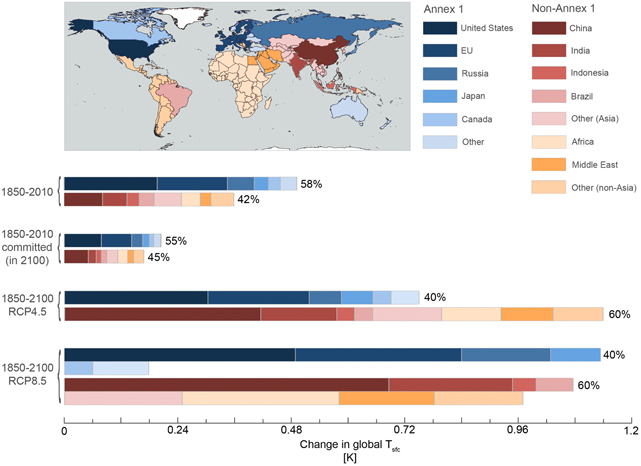
Figure 1. Contributions of Annex I countries (blue colors) and non-Annex 1 countries (red colors) to Δ Ts. Note that values of Δ Ts are affected by our choice of the climate sensitivity, but proportional contributions from countries/regions to the global Δ Ts are not affected by this choice.
Download figure:
Standard image High-resolution imageThe impact of the United States and China is emphasized when countries are viewed individually (figure 2). The United States stands out as the largest historical cause of Δ Ts (figures 2(a), (b)) but is committed at 2050 or 2100 to less than half of its 2010 contribution (figures 2(c), (d)). In contrast, the commitment at 2050 or 2100 from China is only slightly smaller than its 2010 contribution, a result of the cooling from aerosols masking the positive RF from greenhouse gas emissions (figures 2(c), (d)). Both future scenarios include global reductions in aerosol emissions by the mid-21st century (Wise et al 2009, Riahi et al 2007), essentially removing much of the masking effect of aerosols. China and India emerge as major sources of Δ Ts by 2100 in these projections with the two largest sources globally, China and the United States, projected to contribute 35 to 40% of the Δ Ts (figures 2(e), (f)).
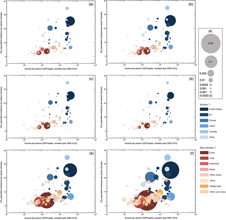
Figure 2. Individual country contributions to Δ Ts for (a) 1850–1990, (b) 1850–2010, (c) committed Δ Ts at 2050, (d) committed Δ Ts at 2100, (e) Δ Ts at 2100 for RCP4.5, and (f) Δ Ts at 2100 for RCP8.5. Values of Δ Ts are indicated by bubble and square area. The bubbles are plotted on a grid of per capita GDP (year 2007) against per capita cCO2-eq (1850–2010, year 2007 population, computed as in den Elzen et al (2013) but without F-gases) to depict the present day differences between Annex 1 and non-Annex 1 countries. Note that values of Δ Ts are affected by our choice of the climate sensitivity, but proportional contributions from countries/regions to the global Δ Ts are not affected by this choice.
Download figure:
Standard image High-resolution imageDen Elzen et al (2013) report that developed countries contributed 52% of global, cumulative CO2-eq (cCO2-eq) emissions between 1850 and 2010. The CO2-eq metric weights emissions of different species by their potential climate impacts. The impacts from a unit emission of a particular forcing agent, with impacts defined using an emissions-based global mean metric, such as the global warming potential (GWP) (Fuglestvedt et al 2003), is equated with the emissions of CO2 that have the same impacts. Den Elzen et al (2013) compute CO2-eq for CO2, CH4, N2O and F-gas emissions using GWPs for each species calculated with a time horizon of 100 years. We compare their results to the proportion of Δ Ts attributable to each country/region (table 1). The United States emitted less than 20% of global cCO2-eq between 1850 and 2010 but accounts for 23% of the Δ Ts. In contrast, Africa and China together emitted about the same amount of cCO2-eq as the United States during this period, but only contributed 14% of the Δ Ts.
Table 1. Percentage of global cumulative CO2-equivalent emissions (cCO2-eq: GWPs calculated with a time horizon of 100 years) (den Elzen et al 2013) and ΔTs for the period 1850–2010 contributed by the list of countries and regions.
| Annex 1 | Non-Annex 1 | ||||
|---|---|---|---|---|---|
| Region | %cCO2-eq | %ΔTs | Region | %cCO2-eq | %ΔTs |
| United States | 18.6 | 23.1 | China | 11.6 | 9.6 |
| European Union | 17.1 | 17.4 | India | 4.1 | 6.0 |
| Russia | 7.2 | 6.7 | Indonesia | 4.8 | 3.1 |
| Japan | 2.8 | 3.5 | Brazil | 3.9 | 3.7 |
| Canada | 1.9 | 3.0 | Other (Asia) | 7.8 | 6.7 |
| Other | 4.3 | 4.1 | Africa | 7.1 | 4.7 |
| — | — | — | Middle east | 3.0 | 2.6 |
| — | — | — | Other (non-Asia) | 5.9 | 5.7 |
| Total | 51.9 | 57.8 | Total | 48.1 | 42.2 |
The differences result from the dissimilar set of forcing agents that dominates in developed and developing countries. Prior to 2010, the RF from Annex-1 countries is essentially a combination of positive CO2 and negative aerosol RFs (figure 3). The magnitude of the remaining forcing agents is minor in comparison. CH4 plays a greater role for non-Annex 1 countries but because of its short lifetime relative to CO2, distant past emissions that are devalued by the Δ Ts metric are weighted equally with current emissions by the CO2-eq metric, as defined by den Elzen et al (2013). Developed countries contribute 30% of the global CH4 cRF from 1850 to 2010, but 70% of the global CO2 cRF. As a result, the Δ Ts is increased relative to the cCO2-eq emissions for Annex 1 countries and reduced for non-Annex 1 countries.
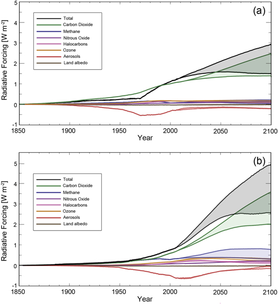
Figure 3. Time series of RF for the forcing agents considered in this study given for (a) Annex 1 countries and (b) non-Annex 1 countries. The shaded areas illustrate the range in RF between the RCP4.5 and RCP8.5 projections.
Download figure:
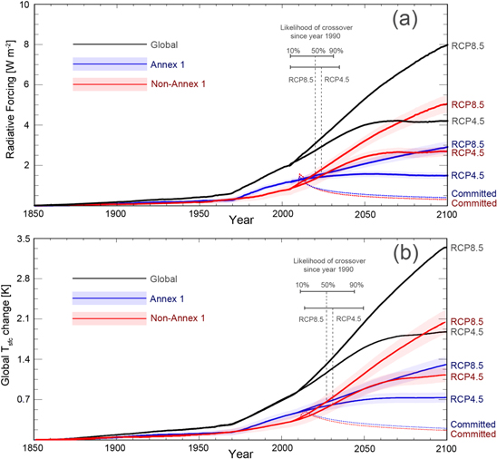
Standard image High-resolution imageThe RF from developing countries, including all forcing agents, is projected to increase rapidly between 2010 and 2050 in both scenarios, while developed countries' impact increases at a smaller rate (figure 3). The result is a role reversal in the future in that the majority of Δ Ts (60%) is ascribed to developing countries in 2100 (figure 4).
Figure 4. Time series of (a) RF and (b) Δ Ts for global anthropogenic emissions and land cover change, and the Annex 1 and non-Annex 1 contributions. Partitioning uncertainty is shown for country group time series. The committed RF and Δ Ts are shown as dotted lines. Note that values of Δ Ts are affected by our choice of the climate sensitivity, but proportional contributions from countries/regions to the global Δ Ts are not affected by this choice.
Download figure:
Standard image High-resolution image
Relative contributions to global temperature change from the greenhouse gas emissions of developed and developing countries have been projected to crossover between years 2010 and 2020 (Höhne et al 2010, den Elzen et al 2013). We estimate the crossover year for Δ Ts with a set of Monte Carlo simulations that output the proportions of the Δ Ts ascribed to Annex 1 countries and non-Annex 1 countries separately for each year starting in 1850. In each Monte Carlo simulation the respective Δ Ts values vary within a Gaussian probability density function centered on the global mean Δ Ts within which the prior computed uncertainties represent one standard deviation. The results give a yearly probability that the non-Annex 1 contribution is greater than the Annex 1 contribution, and the crossover year is defined as the first year in the 21st century when that probability exceeds 0.5. The crossover years for Δ Ts are near 2030 for both projections, implying that Annex 1 countries will account for the majority of climate change for several years after they have become the minority RF contributor (2020 for RCP8.5 and 2024 for RCP4.5), largely because of their dominance of historical greenhouse gas emissions and reduced masking of the warming by aerosols.
4. Discussion
By including aerosols in our analysis we give climate credit to nations that emit high levels of aerosols and may do so at the expense of local air quality (Nemet et al 2010). Similar assessments that use cCO2-eq as a metric attribute climate change to countries without the cooling influence of aerosols and weighting past emissions the same as recent emissions (e.g. Höhne et al 2010, den Elzen et al 2013), providing a different perspective on this problem. We frame our assessment with the assumption that mitigation of global surface temperature warming is the singular goal, whereas issues of air quality and ecosystem preservation are not considered; in our case the inclusion of the impact of short-lived gases and aerosols and albedo effects will be more accurate. A potential solution for assigning country-level responsibility given both positive and negative forcings could include all historical forcings to assign current responsibility, but not allow negative forcings to offset future emissions. Although, we stress that our characterization of contributions to climate change does not include changes in responsibility for forcings that result from trading, or outsourcing of emissions (Rose et al 1998, Peters et al 2012), deductions for greenhouse gas emissions that are required to meet a country's basic needs (Müller et al 2009) or to develop technology with global benefits (den Elzen et al 2013).
Including aerosol indirect effects in our assessment of country contributions allows for a more complete analysis compared to previous studies, but also introduces larger uncertainties into our analysis. To test the sensitivity of our results to this uncertainty, we scale global aerosol indirect effect ERF in an additional set of MAGICC6 simulations with the country-level RF timeseries, applying a scaling factor that ranges between zero and two. The targeted scaling impacts the proportional contribution of China the most (table 2). Major aerosol emitters benefit from weighting this forcing higher, while developed countries for which aerosol emissions are declining (e.g. United States, European Union) see their contribution increase as the weighting increases. The range of scaling from zero to two roughly captures the confidence interval around the central estimate of the indirect effect ERF reported by Myhre et al (2013).
Table 2. Percentage contribution to ΔTs between 1850 and 2010 attributed to the countries and regions listed, computed by MAGICC6 when the aerosol indirect effect is scaled by a range of factors (S). Here 'AX1' is used for Annex 1 and 'NX1' for non-Annex 1.
| Contribution to ΔTs 1850–2010 [%] | |||||
|---|---|---|---|---|---|
| Country/Region | S = 0.0 | S = 0.5 | S = 1.0 | S = 1.5 | S = 2.0 |
| United States | 19 | 21 | 23 | 27 | 34 |
| European Union | 15 | 16 | 17 | 20 | 23 |
| China | 13 | 12 | 10 | 6 | 0 |
| Other NX1 (Asia) | 7 | 7 | 7 | 6 | 6 |
| Russia | 6 | 6 | 7 | 7 | 8 |
| India | 6 | 6 | 6 | 6 | 6 |
| Other NX1 (non-Asia) | 6 | 6 | 6 | 5 | 4 |
| Africa | 6 | 6 | 5 | 3 | 0 |
| Other AX1 | 4 | 4 | 4 | 4 | 4 |
| Brazil | 4 | 4 | 4 | 4 | 4 |
| Japan | 3 | 3 | 4 | 4 | 4 |
| Indonesia | 3 | 3 | 3 | 3 | 2 |
| Canada | 3 | 3 | 3 | 3 | 4 |
| Middle East | 3 | 3 | 3 | 2 | 1 |
| Annex 1 countries | 50 | 53 | 58 | 65 | 77 |
| non-Annex 1 countries | 50 | 47 | 42 | 35 | 23 |
Developing countries are projected to overtake developed countries in their contributions to Δ Ts, we estimate near year 2030. Yet, at present and in the future projections, a few countries, the United States, China, India, and the European Union combined account for more than half of the Δ Ts (figure 1). This result is independent of the range in aerosol indirect effects tested here (table 2) and lends support to calls for alternate grouping of countries in differentiating responsibilities for climate change mitigation (e.g. Parikh and Baruah 2012), although there are important economic considerations that we do not account for. Whether or not the Annex groupings are maintained, our results provide a comprehensive assessment of individual country contributions to climate change that goes beyond greenhouse gas emissions and can inform decision-makers such as the UNFCCC seeking to assign responsibility for current climate change to construct effective, yet equitable, future emissions agreements.
Acknowledgements
We acknowledge support from the National Science Foundation (NSF) AGS-1049033 and the Guggenheim Foundation and are grateful for the valuable feedback from three anonymous referees. Model integrations were performed with a National Center for Atmospheric Research facility, which is sponsored by the NSF.