
Abstract
The land-use sector can contribute to climate change mitigation not only by reducing greenhouse gas (GHG) emissions, but also by increasing carbon uptake from the atmosphere and thereby creating negative CO2 emissions. In this paper, we investigate two land-based climate change mitigation strategies for carbon removal: (1) afforestation and (2) bioenergy in combination with carbon capture and storage technology (bioenergy CCS). In our approach, a global tax on GHG emissions aimed at ambitious climate change mitigation incentivizes land-based mitigation by penalizing positive and rewarding negative CO2 emissions from the land-use system. We analyze afforestation and bioenergy CCS as standalone and combined mitigation strategies. We find that afforestation is a cost-efficient strategy for carbon removal at relatively low carbon prices, while bioenergy CCS becomes competitive only at higher prices. According to our results, cumulative carbon removal due to afforestation and bioenergy CCS is similar at the end of 21st century (600–700 GtCO2), while land-demand for afforestation is much higher compared to bioenergy CCS. In the combined setting, we identify competition for land, but the impact on the mitigation potential (1000 GtCO2) is partially alleviated by productivity increases in the agricultural sector. Moreover, our results indicate that early-century afforestation presumably will not negatively impact carbon removal due to bioenergy CCS in the second half of the 21st century. A sensitivity analysis shows that land-based mitigation is very sensitive to different levels of GHG taxes. Besides that, the mitigation potential of bioenergy CCS highly depends on the development of future bioenergy yields and the availability of geological carbon storage, while for afforestation projects the length of the crediting period is crucial.
Export citation and abstract BibTeX RIS

Content from this work may be used under the terms of the Creative Commons Attribution 3.0 licence. Any further distribution of this work must maintain attribution to the author(s) and the title of the work, journal citation and DOI.
Introduction
For ambitious climate change mitigation, huge reductions in greenhouse gas (GHG) emissions are needed (Meinshausen et al 2009, Rogelj et al 2011, 2013a). Currently, the land-use sector is responsible for 17–32% of global anthropogenic GHG emissions (Bellarby et al 2008). There are several measures for reducing GHG emissions in the land-use sector, such as avoided deforestation or improved agricultural management (Smith et al 2013). However, the land-use sector cannot only contribute to climate change mitigation by decreasing GHG emissions, but also by increasing carbon uptake from the atmosphere (Rose et al 2012). Recent integrated assessment modeling (IAM) studies focused on afforestation and bioenergy in combination with carbon capture and storage (bioenergy CCS) as land-based mitigation strategies for carbon removal (Tavoni and Socolow 2013). Both strategies make use of the accumulation of carbon in growing biomass through photosynthesis. Bioenergy CCS removes carbon from the atmosphere by capturing the carbon released during the combustion of biomass and storing the captured carbon in geological reservoirs underground. Afforestation detracts carbon from the atmosphere through the managed regrowth of natural vegetation. While carbon removal due to bioenergy CCS can be raised through land expansion and yield increases (increase in productivity per unit area), gains in carbon removal due to afforestation are mostly limited to the extensification of forestland.
In the literature, studies focus on the standalone mitigation potential of bioenergy CCS (Azar et al 2010, Popp et al 2011, Klein et al 2014, Kriegler et al 2013, Vuuren et al 2013) and afforestation (Strengers et al 2008, Reilly et al 2012) or investigate both at the same time (Wise et al 2009, Calvin et al 2014, Edmonds et al 2013). However, the standalone and combined effects of bioenergy CCS and afforestation on land-use and carbon dynamics have not been analyzed so far with a common methodological approach. Looking at both, the standalone and combined mitigation potential, provides insight into potential trade-offs like competition for land or path dependencies, which are important for the evaluation of afforestation and bioenergy CCS as mitigation strategies. In this study, we use the Model of Agricultural Production and its Impacts on the Environment (MAgPIE), a spatially explicit, global land-use model to analyze three scenarios with different land-based mitigation policies: afforestation, bioenergy CCS and the combination of both. Land-based mitigation in MAgPIE is incentivized by an exogenously given tax on GHG emissions. The trade-off between land expansion and yield increases is treated endogenously in the model. In order to test the stability of our results, we perform sensitivity analyses with the most important exogenous parameters.
Methods and material
Land-use model MAgPIE
MAgPIE is a spatially explicit, global land-use allocation model and projects land-use dynamics in ten-year time steps until 2095 using recursive dynamic optimization (Lotze-Campen et al 2008, Popp et al 2010). The objective function of MAgPIE is the fulfilment of food, livestock and material demand at minimum costs under socio-economic and biophysical constraints. Demand is based on exogenous future population and income projections (see scenario section), while price-induced changes in consumption are not reflected. Major cost types in MAgPIE are: factor requirement costs (capital, labor and fertilizer), land conversion costs, transportation costs to the closest market, costs for R&D (technological change) and costs for GHG emission rights. For long term investments, like land conversion or R&D, we assume a time horizon of 30 years and an annual discount rate of 7%, which reflects the opportunity costs of capital at the global level (IPCC 2007, chapter 2.4.2.1). While socio-economic constraints like trade liberalization and forest protection are defined at the regional level (ten world regions) (figure S1), biophysical constraints such as crop yields, carbon density and water availability, derived from the global hydrology and vegetation model LPJmL (Bondeau et al 2007, Müller and Robertson 2014), as well as land availability (Krause et al 2013), are introduced at the grid cell level (0.5 degree longitude/latitude; 59 199 grid cells). Due to computational constraints, all model inputs in 0.5 degree resolution are aggregated to 500 clusters for the optimization process based on a k-means clustering algorithm (Dietrich et al 2013). During the optimization process, the cluster level is the finest resolution. The clustering algorithm combines grid cells to clusters based on the similarity of data for each of the ten world regions. If, for instance, two grid cells with similar land patterns are merged into one cluster, the algorithm preserves the land area available by summing up the area of the two grid cells. Investment in R&D in the agricultural sector translating into yield-increasing technological change is a variable in MAgPIE and can therefore endogenously enhance food and bioenergy crop yields (Dietrich et al 2014). Finally, the cost minimization problem is solved through endogenous variation of spatial production patterns, land expansion (both at the cluster level) and yield-increasing technological change (at the regional level) (Lotze-Campen et al 2010).
MAgPIE features land-use competition based on cost-effectiveness at cluster level among the land-use related activities food, livestock and bioenergy production as well as afforestation. Available land types are cropland, pasture, forest and other land (e.g. non-forest natural vegetation, abandoned agricultural land, desert). The forestry sector, in contrast to the agricultural and livestock sector, is currently not implemented dynamically in MAgPIE. Therefore, timberland needed for wood production, consisting of forest plantations and modified natural forest, is excluded from the optimization, which is about 30% of the initial global forest area (4235 mio ha). In addition, other parts of forestland, mainly undisturbed natural forest, are within protected forest areas, which is about 12.5% of the initial global forest area (FAO 2010). Altogether, about 86% of the world's land surface is freely available in the optimization of the initial time-step.
MAgPIE calculates emissions of the Kyoto GHGs carbon dioxide (CO2), nitrous oxide (N2O), and methane (CH4) (Bodirsky et al 2012, Popp et al 2010, 2012). Mitigation of GHG emissions is stimulated by an exogenous tax regime on GHG emissions (see scenario section). The GHG tax is multiplied with GHG emissions in order to calculate GHG emission costs, which enter the cost minimizing objective function of MAgPIE. For instance, CO2 emissions from land-use change can be reduced through avoided deforestation (carbon stock conservation). But unlike N2O and CH4 land-use emissions, CO2 emission from the land-use system can become negative if photosynthetic carbon uptake from the atmosphere outweighs carbon release to the atmosphere from plant decomposition and land-use change (carbon stock increase). Therefore, land-based climate change mitigation via afforestation or bioenergy CCS is incentivized by the revenue from the GHG tax regime for carbon removal from the atmosphere. A detailed description of the underlying formulas is available in the supplementary data, available at stacks.iop.org/ERL/0/000000/mmedia. For the conversion of N2O and CH4 emissions into CO2eq we use GWP100 (IPCC (2013)).
Bioenergy CCS
In MAgPIE, dedicated lignocellulosic biomass (rainfed only) can be converted to secondary energy via different conversion routes. The carbon released from biomass during combustion is captured and stored underground using CCS technology.
Herbaceous and woody bioenergy yields at grid cell level for the initialization of MAgPIE are derived from LPJmL (Beringer et al 2011). While LPJmL simulations supply data on potential yields, i.e. yields achieved under the best currently available management options, MAgPIE aims to represent actual yields. Therefore, LPJmL yields are reduced using information about observed land-use intensity (Dietrich et al 2012) and agricultural area (FAO 2013). For instance, in China (CPA) herbaceous bioenergy yields from LPJmL are reduced by about 45% to obtain actual yields for the initialization of MAgPIE (table 1). MAgPIE bioenergy yields can exceed LPJmL bioenergy yields over time as endogenous investments in R&D push the technology frontier. Higher bioenergy yields are associated with increased carbon uptake from the atmosphere per unit area.
Table 1. Regional herbaceous bioenergy yields (GJ ha−1) in 1995 derived from LPJmL (potential yields) and initial bioenergy yields MAgPIE (actual yields). Region specific yields are obtained by calculating the average across all clusters within a region.
| AFR | CPA | EUR | FSU | LAM | MEA | NAM | PAO | PAS | SAS | |
|---|---|---|---|---|---|---|---|---|---|---|
| LPJmL | 198 | 188 | 165 | 59 | 382 | 26 | 101 | 154 | 595 | 235 |
| MAgPIE | 52 | 105 | 125 | 21 | 150 | 9 | 71 | 48 | 251 | 110 |
Bioenergy CCS can provide energy and remove carbon from the atmosphere at the same time. Due to this versatility, bioenergy CCS is an attractive mitigation option in scenarios with ambitious climate targets. The largest share of profits in these scenarios comes from the carbon sequestration and not from the energy portion of the bioenergy CCS technology (Rose et al 2014). In this study, we focus on the carbon removal potential of bioenergy CCS and therefore disregard the value of the energy produced. We implemented three different conversion routes with CCS technology in the model: biomass to hydrogen (B2H2), biomass integrated gasification combined cycle and biomass to liquid (B2L) (Klein et al 2014). Levelized costs of energy (LCOEs) are calculated using the time horizon of 30 years and the discount rate of 7% (see MAgPIE description), which are both within the range of common assumptions for LCOE calculations (IEA and OECD NEA 2010, chap 2.3). The LCOEs include initial investment costs in infrastructure as well as operational and maintenance costs. The B2H2 technology in combination with CCS features a higher conversion efficiency (55%) and carbon capture rate (90%) at lower LCOEs (8 $ GJ−1) than the other available technologies (based on Klein et al 2014). Demand for bioenergy in this study does not rely on exogenous trajectories, but is derived endogenously as a response to the GHG tax, which rewards carbon removal due bioenergy CCS, while the value of energy produced due to bioenergy CCS is disregarded. The cost minimizing objective function of MAgPIE in combination with carbon removal being the only incentive in the model to employ bioenergy CCS renders the B2H2 technology superior to the other available conversion routes. The geological carbon storage capacity is constrained at the regional level (table S3), which adds up to 3960 GtCO2 at the global level (Bradshaw et al 2007). We assume a lifetime of the CCS technology of 200 years (Szulczewski et al 2012) and therefore limit the annual geological injection of carbon to 0.5% yr–1 in terms of the geological carbon storage capacity, which results in an annual realizable geological injection rate of about 20 GtCO2 yr–1 globally. As biomass can be traded, the location of geological carbon storage can differ from the location of biomass production. Levelized costs for transportation and injection of captured carbon are at 9 $/tCO2 (Klein et al 2014).
Afforestation
Compared to bioenergy CCS, afforestation can be considered as low-tech land-based mitigation strategy, since no technical infrastructure for processing is needed. In MAgPIE, afforestation is a managed regrowth of natural vegetation. The regrowth is managed in that way as endemic seed sources are put in place manually as part of the land conversion process. Regrowth of natural vegetation affects vegetation, litter and soil carbon stocks, which are calculated as the product of carbon density and afforestation area (see online supplementary data for details). Vegetation, litter and soil carbon density of potential natural vegetation in 1995 at grid cell level is derived from LPJmL (figure S4). Vegetation carbon density increases over time along S-shaped growth curves (figure 1). The vegetation carbon density growth curves are based on a Chapman–Richards volume growth model (Murray and von Gadow 1993, Gadow and Hui 2001), which is parameterized using vegetation carbon density of potential natural vegetation (figure S4(a)) and climate region specific mean annual increment (MAI) and MAI culmination age (IPCC 2006). Litter and soil carbon density are assumed to increase linearly towards the value of potential natural vegetation (figures S4(b) and (c)) within a 20 years time frame (IPCC 2000). The initial value for vegetation and litter carbon density is assumed to be 0, while the initial grid-cell specific value for soil carbon density is the average between cropland and potential natural vegetation soil carbon density.

Figure 1. Climate region specific S-shaped vegetation carbon density growth curves for a period of 100 years. The vertical axis presents the share of grid-cell specific vegetation carbon density of potential natural vegetation in 1995 (figure S4a).
Download figure:
Standard image High-resolution imageIn MAgPIE, the decision to invest in afforestation depends on the benefit-cost ratio over the time horizon of 30 years, which is a common crediting period for afforestation projects (United Nations 2013). Firstly, cumulative carbon uptake over the time horizon is calculated as the product of new afforestation area and carbon density (vegetation, litter and soil) at age 30. Secondly, the benefit of an afforestation activity is calculated as the product of this cumulative carbon uptake 30 years ahead and the level of the current GHG tax (see online supplementary data for more details). Finally, for comparability with the annual bioenergy CCS activity, this future cash flow is annualized using the discount rate of 7% (see MAgPIE description). Land conversion and management costs are based on Sathaye et al (2005). Regional costs for the conversion of any land type into afforestation land range between 849 $ ha−1 (SAS) and 2484 $ ha−1 (NAM) (table S2) in the initial time step and are proportionally scaled with GDP for future time steps. Total land conversion costs are annualized. Annual management costs range between 2 $ ha–1 yr–1 (FSU) and 127 $ ha–1 yr–1 (AFR). Contrary to bioenergy CCS, technological change has no direct effect on the carbon removal potential of afforestation.
Scenarios
Our scenarios are based on the shared socio-economic pathways (SSPs) for climate change research (O'Neill et al 2014). It should be noted that the SSPs do not incorporate climate mitigation policies by definition. In this study, we choose SSP 2, a 'Middle of the Road' scenario with intermediate socio-economic challenges for adaptation and mitigation. Food, livestock and material demand (figure S2) is calculated using the methodology described in Bodirsky et al and the SSP 2 population and GDP projections (IIASA 2013).
We assume a GHG tax (Tax30) on Kyoto gases (CO2, N2O, CH4) that increases nonlinearly at a rate of 5% yr–1 (Kriegler et al 2013). The GHG tax has a level of 30 $/tCO2eq in 2020 and starts in 2015 (figure S3). The resulting GHG tax with prices of 102 $/tCO2eq in 2045 and 1165 $/tCO2eq in 2095 is close to GHG price trajectories required to limit global average temperature increase to 2 °C above pre-industrial levels with a probability of 50% (Rogelj et al 2013b). Due to this ambitious climate change mitigation target, biophysical climate impacts on crop yields and carbon densities are assumed to be weak and are therefore not regarded in this study.
We investigate four scenarios, which cover two dimensions: GHG tax and availability of carbon removal options (table 2). In the business as usual scenario (BAU), no tax on GHG emissions is applied, i.e. there is no incentive to avoid GHG emissions. In the mitigation scenarios, the GHG tax penalizes all positive GHG emissions from the land-use system and rewards negative CO2 emissions from afforestation in AFF, from bioenergy CCS in BECCS, and from both in AFF+BECCS.
Table 2. Scenario definitions; GHG tax: Tax30 has a level of 30 $/tCO2eq in 2020, starts in 2015 and increases by 5% yr–1; carbon removal option(s): available option(s) for generating negative CO2 emissions rewarded by the GHG tax.
| GHG tax | Carbon removal option(s) | |
|---|---|---|
| BAU | — | — |
| AFF | Tax30 | Afforestation |
| BECCS | Tax30 | Bioenergy CCS |
| AFF+BECCS | Tax30 | Afforestation and bioenergy CCS |
Sensitivity analysis
To address the uncertainty in exogenous model parameters, we investigate the sensitivity of our simulations to changes in model parameterization. Crucial parameters in the context of this study are the geological carbon storage capacity (CCS capacity), the GHG tax, the time horizon for investment decisions, the discount rate, and assumptions about future bioenergy yields. Table 3 summarizes the parameter settings for the sensitivity analysis.
Table 3. Parameter settings for sensitivity analysis. 'DEFAULT' characterizes our default parameter settings used in this study. 'LOW'/'HIGH' characterize lower/higher parameter values compared to 'DEFAULT'.
| CCS capacity globally | GHG tax in 2020 (2095) | Time horizon | Discount rate | Bioenergy yields | |
|---|---|---|---|---|---|
| [Gt CO2] | [US$/tCO2eq] | [Years] | [% yr–1] | [−] | |
| LOW | 198 | 5 (194) | 10 | 4 | Static |
| DEFAULT | 3960 | 30 (1165) | 30 | 7 | Variable |
| HIGH | 79200 | 50 (1942) | 50 | 10 | — |
CCS capacity: Bradshaw et al (2007) estimates a range for geological carbon storage capacity at the global level of 100–200 000 GtCO2. For DEFAULT, we use 3960 GtCO2. For the sensitivity analysis we vary this value by factor 20 in both directions (198 GtCO2 in LOW, 79 200 GtCO2 in HIGH). Based on Szulczewski et al (2012), we assume a lifetime of CCS of 200 years. Therefore, we limit the annual injection of carbon to 0.5% yr–1 in terms of the total CCS capacity. For DEFAULT this results in 20 GtCO2 of the total CCS capacity, for LOW in 1 GtCO2 yr–1 and for HIGH in 396 GtCO2 of the total CCS capacity globally.
GHG tax: in DEFAULT, the GHG tax has a level of 30 $/tCO2eq in 2020, starts in 2015 and increases by 5% yr–1. For LOW and HIGH, the level of the GHG tax is 5 and 50 $/tCO2eq in 2020 respectively. The range for the sensitivity analysis is based on Kriegler et al (2013).
Time horizon: in DEFAULT, the time horizon for investments is 30 years, which is common in the energy sector as well as for afforestation projects. For LOW and HIGH we chose 10 and 50 years respectively (IEA and OECD NEA 2010, United Nations 2013).
Discount rate: in DEFAULT, the annual discount rate is 7%, which reflects the opportunity costs of capital at the global level. For the sensitivity analysis, we vary the discount rate by 3% points in both directions, based on a literature range of 4–12% (IPCC (2007), chap 2.4.2.1).
Bioenergy yields: in DEFAULT, bioenergy yields are variable and assumed to increase, along with food crop yields, due to endogenous technological change in the agricultural sector. In LOW, technological change in the agricultural sector has no impact on bioenergy crop yields (i.e. bioenergy yields are fixed at the initial level), while food crop yields can still increase due to technological change.
To investigate the role of the algorithm used for clustering our high resolution input data, we perform sensitivity analysis with different numbers of spatial cluster units (100–500) in addition.
Results
Land-use dynamics
In 1995, total land cover (12 907 mio ha) consists of food crop (1425 mio ha), pasture (3073 mio ha), forest (4235 mio ha) and other land (4174 mio ha) (figure 2). In the BAU scenario (no GHG tax), food crop area increases by about 300 mio ha until 2095, mainly at the expense of forestland. In the second half of the century, pasture area decreases due to stabilizing livestock demand (figure S2) in combination with average yield increases of about 0.48% yr–1 (figure S10), leading to an increase of abandoned agricultural land. In the mitigation scenarios, the GHG tax on land-use change emissions keeps forestland almost constant over time. Afforestation emerges as cost-efficient mitigation strategy from 2015 (start of GHG tax at 24 $/tCO2eq) and increases, mainly at the expense of pasture and food crop area, to 2773 mio ha in AFF until 2095. Endogenous yield increases, accompanied by changes in spatial production patterns, compensate for the reduced agricultural area. In AFF, the cost–efficient level of average yield increases in the agricultural sector is 1.21% yr–1 throughout the 21st century (figure S10). Bioenergy CCS comes into play much later than afforestation, as it is cost-efficient first in 2065 (270 $/tCO2eq). Bioenergy area increases to 508 mio ha until 2095 in BECCS, mainly at the expense of food crop area. Total dedicated bioenergy production, mainly herbaceous crops, stabilizes at 237 EJ yr–1 until 2095 (figures S6, S7). In the combined setting, AFF+BECCS, afforestation area (2566 mio ha) is slightly smaller compared to AFF, while bioenergy area (300 mio ha) is almost halved compared to BECCS. Despite the smaller bioenergy area, bioenergy production remains at 237 EJ yr–1 in 2095 in AFF+BECCS, which is reflected in a higher level of average yield increases in AFF+BECCS (1.37% yr–1) compared BECCS (1% yr–1) (figure S10).

Figure 2. Time-series of global land-use pattern (109 ha) for BAU, AFF, BECCS and AFF+BECCS and six land types.
Download figure:
Standard image High-resolution imageThe maps in figure 3 illustrate the spatial distribution of afforestation and bioenergy area for the standalone scenarios (AFF/BECCS) and the combined setting (AFF+BECCS) in 2095. In the standalone scenarios, afforestation area is found in many world regions, predominantly in Sub-Sahara African, Latin America, China, Europe and the USA, while bioenergy area is mostly found in the northern hemisphere in the USA, China and Europe. In the combined scenario, afforestation area is similar to AFF. But due to competition for land between the two carbon removal options, afforestation area is reduced in favor of bioenergy area in the USA and China in AFF+BECCS. There are several reasons why the USA, China and Europe are the main bioenergy producers. We provide insight in subsection 'Bioenergy CCS and the role of yield increases' along with figure 5.
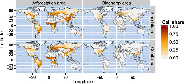
Figure 3. Grid-cell specific share of afforestation and bioenergy area in the standalone scenarios (top) and the combined setting (bottom) in 2095. Colors indicate the share of afforestation or bioenergy area in each cell. Grid-cell specific results are obtained by disaggregation of cluster level results (each grid cell is assigned the value of the cluster it belongs to).
Download figure:
Standard image High-resolution imageCarbon dynamics
In the BAU scenario, CO2 emissions from the land-use system accumulate to 177 GtCO2 until 2095 (figure 4). The peak in mid-century is mainly caused by deforestation, while the following decline in CO2 emissions is due to ecological succession on abandoned agricultural land. In the mitigation scenarios, the described land-use dynamics lead to net carbon removal from the atmosphere. More precisely, carbon is detracted from the atmosphere by photosynthesis and is either biologically sequestered via afforestation or geologically sequestered via bioenergy CCS. In AFF, land conversion into afforestation area increases cumulative CO2 emissions in 2015, followed by continuous carbon removal of about 10 GtCO2 yr–1 throughout the 21st century. Until 2095, carbon removal in AFF accumulates to 703 GtCO2. In BECCS, cumulative CO2 emissions are almost constant until bioenergy CCS becomes cost-efficient as mitigation strategy in 2065 at GHG prices of 270 $/tCO2eq. From 2065, carbon removal in BECCS is about 20 GtCO2 yr–1, which cumulates to 591 GtCO2 until 2095. In AFF+BECCS, carbon dynamics are similar to AFF until bioenergy CCS becomes competitive as mitigation option in addition to afforestation in 2055. Carbon removal in AFF+BECCS is about 25 GtCO2 yr–1 in from 2065 to 2095, which results in cumulative carbon removal of 1000 GtCO2 until 2095. In 2095 in BECCS and AFF+BECCS, the constraint on the annual geological carbon injection rate is binding (20 GtCO2 yr–1), while cumulative carbon storage capacity (3960 GtCO2) would last for approximately another 150 years.

Figure 4. Time-series of global cumulative N2O and CO2 emissions (GtCO2eq) from the land-use system for BAU, AFF, BECCS and AFF+BECCS.
Download figure:
Standard image High-resolution imageBioenergy CCS and the role of yield increases
Contrary to afforestation, the carbon removal rates per unit area of bioenergy CCS can be enhanced through yield increases. Figure 5 illustrates the potential annual carbon removal rates during the optimization for 1995 and 2095 in the AFF+BECCS scenario, i.e. the annual carbon removal rates shown here represent realizable, but not necessarily realized, carbon removal rates (compare to figure 3). In the remainder of this subsection, we talk about annual realizable carbon removal rates. In 1995, afforestation shows higher carbon removal rates than bioenergy CCS in the majority of cells, with highest carbon removal rates in the tropics (about 20 tC ha–1 yr–1). In 2095, the picture is fundamentally different due to yield-increasing technological change on bioenergy crops, which increases carbon removal per unit area. In AFF+BECCS, average yield-increase throughout the century is at 1.38% yr–1 (figure S10), which more than triples initial bioenergy yields until 2095 (figure S5). By end-of-century bioenergy CCS exceeds the carbon removal rates of afforestation in the tropics (about 25–30 tC ha–1 yr–1). However, bioenergy production does not take place in the tropics but mainly in the USA, China and Europe (figure 3) for three reasons. First of all, the USA and China exhibit higher carbon removal rates in 2095 (about 30–40 tC ha–1 yr–1) compared to the tropics. Second, the tropical regions are the most attractive places for afforestation. Third, bioenergy production relies on transport infrastructure, which is much more sophisticated in Europe, USA and China than in the tropics (Nelson 2008). Bioenergy yield gains go along with increased fertilizer use, which drives N2O emissions. In 2095, cumulative N2O emission in BECCS and AFF+BECCS are about 30–50 GtCO2eq higher compared to BAU or AFF (figure 4), although N2O emissions are penalized by the GHG tax.
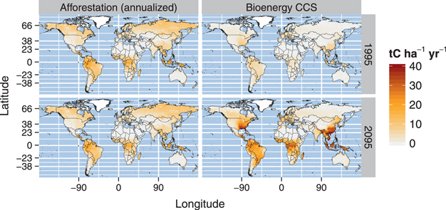
Figure 5. Grid-cell specific illustration of potential annual carbon removal rates from afforestation and bioenergy CCS for 1995 (top) and 2095 (bottom) in the AFF+BECCS scenario (tC ha–1 yr–1). Annual carbon removal due to afforestation is calculated as average annual carbon increase in vegetation, litter and soil over a period of 30 years. Annual carbon removal due to bioenergy CCS is based on B2H2 conversion technology in combination with dedicated herbaceous bioenergy crops. Bioenergy yields are converted to carbon densities using a conversion factor of 0.45 t C/t DM. Grid-cell specific results are obtained by disaggregation of cluster level results (each grid cell is assigned the value of the cluster it belongs to).
Download figure:
Standard image High-resolution imageSensitivity analysis
In order to test the stability of our results, we perform sensitivity analyses with crucial exogenous parameters (table 3). Figure 6 shows the results in terms of land and carbon dynamics at the global level. Regional results can be found in figure S8.
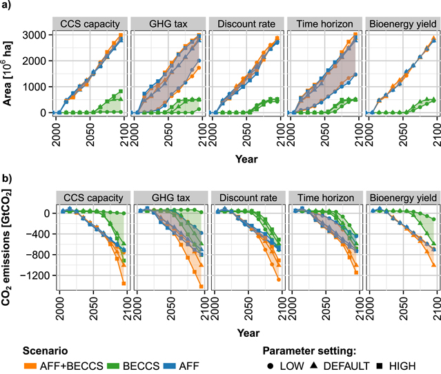
Figure 6. Time-series of sensitivity analysis for AFF, BECCS and AFF+BECCS at the global level. The settings (LOW, DEFAULT, HIGH) for the different parameters (CCS capacity, GHG tax, discount rate, time horizon, bioenergy yield) are described in table 3. The shaded areas span the whole range of sensitivity in the respective scenario in terms of (a) area in use for land-based mitigation (106 ha) and (b) cumulative CO2 emissions (GtCO2).
Download figure:
Standard image High-resolution image
The constraint on the annual geological carbon injection rate is crucial for the scenarios with bioenergy CCS. With 1 GtCO2 yr–1 and 20 GtCO2 yr–1 the constraint is binding, which indicates that the mitigation potential of bioenergy CCS is mostly limited by the annual geological carbon injection rate. However, with a potential of 396 GtCO2 yr–1 the constraint is not binding, which indicates that the potential of bioenergy CCS is also limited by other factors like land availability and costs associated with bioenergy production. Bioenergy production is 530 EJ yr–1 in HIGH, compared to 237 EJ yr–1 in DEFAULT and 4 EJ yr–1 in LOW (figure S7). In the combined setting, AFF+BECCS, land demand is similar for all parameter settings, while the difference in carbon removal is about 500 GtCO2. This can be explained by considering that in the combined setting in HIGH average annual yield increases are at 1.5% yr–1 compared to 1.25% yr–1 in LOW (figure S10).
The carbon removal potential is highly sensitive to different levels of the GHG tax, which is the only driver for land-based mitigation in this study. In general, different GHG tax trajectories influence the point in time when bioenergy CCS and afforestation are cost-efficient, which translates into different mitigation potentials in 2095. While bioenergy CCS is cost-efficient starting from carbon prices of 165 $/tCO2eq, afforestation emerges as cost-efficient at prices of 6 $/tCO2eq. Therefore, the impact of changes in the GHG tax trajectory on the mitigation potential is higher in scenarios with bioenergy CCS. In AFF+BECCS, the range of sensitivity for the mitigation potential is about 900 GtCO2. In general, the degree of sensitivity decreases with higher GHG tax levels, especially for afforestation.
Lower annual discount rates (4%) mostly affect the carbon removal potential of bioenergy CCS as lower discount rates facilitate long term investments in R&D translating into agricultural yield increases. On the contrary, higher discount rates (10%) increase the charges for credit, which is reflected in average annual technological change rates of 1.25% yr–1 in HIGH and 1.45% yr–1 in LOW (figure S10). The range of sensitivity for the mitigation potential is about 200 GtCO2 for BECCS and 300 GtCO2 for AFF+BECCS.
In terms of land, the time horizon for investment decisions mostly affects afforestation. With a time horizon of ten years, afforestation area accumulates to about 1500 mio ha, while with a time horizon of 30 or 50 years afforestation area is about 3000 mio ha, which translates into a difference in carbon removal of about 300 GtCO2. The sensitivity of afforestation to the time horizon can be explained by recalling the shape of the forest growth curves in figure 3. The mitigation potential of bioenergy CCS is also affected as a shorter lifetime of investments in CCS infrastructure increases the costs associated with bioenergy CCS.
When bioenergy yields are fixed at their initial level, bioenergy CCS is less attractive as mitigation strategy. In BECCS, bioenergy production is reduced to 74 EJ yr–1 in LOW compared to 237 EJ yr–1 in DEFAULT, which results in a reduction of the mitigation potential of about 500 GtCO2 until 2095. In the combined setting, AFF+BECCS, bioenergy CCS is no longer competitive with afforestation when bioenergy yield are not allowed to increase in the future, which reduces the mitigation potential in LOW compared to DEFAULT by about 300 GtCO2.
The range of sensitivity across different numbers of spatial cluster units (100–500) during the optimization is small for AFF and BECCS (∼50 GtCO2), while it is more pronounced in the combined setting (∼200 GtCO2). In general, we observe a small trend towards less carbon removal with a higher number of cluster units (figure S12).
Discussion and conclusion
In this paper, we investigated the cumulative carbon removal potential in the land-use sector for climate change mitigation scenarios with different land-based mitigation strategies: afforestation, bioenergy CCS and the combination of both. In addition, we tested the sensitivity of our result to changes in crucial exogenous parameters.
As single mitigation strategy, afforestation is cost-efficient at relatively low carbon prices (6 $/tCO2eq), while bioenergy CCS only becomes competitive at higher carbon prices (165 $/tCO2eq). It should be noted that the value of energy produced via bioenergy CCS is disregarded in this study. Instead, the revenue from the GHG tax for carbon removal is considered as the only driver for bioenergy CCS and afforestation. By end-of-century, global area for land-based climate change mitigation is more than five times larger in case of afforestation (∼2800 mio ha) compared to bioenergy CSS (∼500 mio ha). For bioenergy CCS, our area estimates are comparable to recent IAM studies aiming at ambitious climate change mitigation (Popp et al 2014). In general, the limiting factor for land-based mitigation is the availability of land. Besides that, bioenergy production for use with CCS technology is capped by the annual realizable geological carbon injection. Therefore, bioenergy production stabilizes at 237 EJ yr–1 by end-of-century, which is within the range of estimated bioenergy deployment levels until 2050 (Chum et al 2011). Despite the dissimilarities in land demand, cumulative carbon removal by end-of-century is similar for afforestation (703 GtCO2) and bioenergy CCS (591 GtCO2). This can be explained by considering that, contrary to afforestation, yield-increasing technological change can enhance carbon removal per unit area of bioenergy CCS—at the expense of additional N2O emission due to increased fertilizer use, which reduces the mitigation effect of bioenergy CCS throughout the century by about 30–50 GtCO2eq. In addition, both options, afforestation and bioenergy CCS, benefit from area reductions in the agricultural sector due to yield increases. Based on several IAM studies, Tavoni and Socolow (2013) identify a range for cumulative carbon removal until 2100 of 200–700 GtCO2 for afforestation and of 460–910 GtCO2 for bioenergy CCS. Our estimates for afforestation are at the upper end of this range, while for bioenergy CCS estimates are in the middle. The combination of afforestation and bioenergy CCS leads to higher cumulative carbon removal (1000 GtCO2 in AFF+BECCS) compared to scenarios with single mitigation strategies. But carbon removal in the combined setting is less than the sum of carbon removal in the standalone settings, indicating that afforestation and bioenergy CCS compete for land. Although bioenergy area is halved compared to the standalone setting, biomass production and thereby carbon removal due to bioenergy CCS is maintained—at the cost of additional yield increases. The sensitivity analysis shows that land-based mitigation is very sensitive to different levels of GHG taxes. Different GHG tax trajectories influence the point in time when bioenergy CCS and afforestation are cost-efficient, which results in different mitigation potentials in 2095. Moreover, the mitigation potential of bioenergy CCS highly depends on the development of future bioenergy yields and the availability of geological carbon storage, while for afforestation projects the length of the crediting period is crucial.
Although in 2095 the constraint on annual geological carbon injection is binding (20 GtCO2 yr–1), geological carbon injection could continue for approximately another 150 years at this rate after 2095 until the cumulative carbon storage capacity is exhausted. On the other hand, carbon removal rates due to afforestation can be expected to decline when no more land for afforestation is available and forests reach maturity. Therefore, in the longer run bioenergy CCS could probably remove more carbon from the atmosphere than afforestation. Experimental model runs until 2145 support this hypothesis (figure S11). Zeng (2008), Zeng et al (2013) suggest an alternative carbon sequestration strategy related to afforestation. Trees could be harvested regularly and buried underground in trenches, which would prevent the decomposition of the wood for long periods (100–1000 years). Using this approach, a piece of land could be used several times for afforestation, which would probably increase the competiveness of afforestation as mitigation strategy.
Competition for land mostly takes place in the USA, China and Europe, which are attractive for both mitigation strategies. By end-of-21st-century, afforestation area is found in many world regions, especially in the tropics, while bioenergy production concentrates in the USA, China and Europe. Large-scale land-based mitigation might change the albedo of land surfaces, leading to biophysical impacts on the climate system (Vuuren et al 2013). Specifically in snow-covered areas of the northern hemisphere, reduction of albedo due to afforestation might jeopardize the mitigation effect of carbon removal from the atmosphere, which could result in a net warming effect (Schaeffer et al 2006, Bala et al 2007, Jackson et al 2008, Jones et al 2013). In this study, we disregard such feedbacks on the climate system. According to our results, afforestation area is found in boreal regions that might be affected by the albedo effect. However, carbon removal rates due to afforestation in these regions are low compared to the tropics, where afforestation area is found in large part.
Our results indicate that land-based mitigation primarily expands at the expense of cropland and pastureland as the conversion of forestland or other carbon-rich natural vegetation is not attractive due to the GHG tax. Moreover, timberland is not available for conversion as it is reserved for wood production (about 1270 mio ha globally). When the revenue from carbon removal due to bioenergy CCS or afforestation exceeds the revenue from forestry products, timberland might become a source of feedstock for bioenergy or part of an afforestation project. Moreover, if price-induced changes in consumption would be taken into account, competition between food production and land-based mitigation is likely to reduce food demand due to increasing prices for food production, which would result in more area available for land-based mitigation. Therefore, the area available for land-based mitigation might be underestimated in this study to the extent forestry and agricultural demand could be reduced. However, for bioenergy CCS the constraint on geological carbon injection (20 GtCO2 yr–1 globally) is binding at the end of the 21st century. Hence, more available land is rather to increase carbon removal due to afforestation than due to bioenergy CCS.
In order to maintain the provision of food and feed besides land-based mitigation, yield increases in the agricultural sector would be needed to compensate for the reduction in agricultural land. In addition, the mitigation potential of bioenergy CCS relies on future increases of bioenergy yields. According to our results, land-based mitigation measures would require average annual yield increases of 1–1.38% yr–1 globally throughout the 21st century, which is at the lower end of historic yield increases. In the last 40 years, corn and soybean yields grew at a rate of 1.4–1.8% yr–1 in the USA (Egli 2008). At the global level corn yields increased by a factor of 2.5 between 1961 and 2007 (Edgerton 2009), which translates into average annual yield increases of 2% yr–1. However, it is unclear if these rates of yield increase can be maintained in the future and to which extent bioenergy yields will benefit from future yield-increases in the agricultural sector. On the one hand side, measures that increase the harvestable storage organ carbon pool are specifically designed for conventional crops, while the purpose of dedicated bioenergy crops is maximum carbon accumulation across all carbon pools including stems and leaves. On the other side, conventional crops are already at high breeding levels, while breeding in bioenergy crops just started (Głowacka 2011). For instance, the estimated potential yield increase of miscanthus by 2030 is 100% (Chum et al 2011, p 277). In addition, also the starting point for potential bioenergy yield increases is uncertain. The range of estimates for current lignocellulosic bioenergy yields is 120–280 GJ ha−1 in Europe and 150–415 GJ ha−1 in South America (Chum et al 2011, p 234). While initial bioenergy yields in MAgPIE are at the lower end of these estimates (125 GJ ha−1 in Europe, 150 GJ ha−1 in Latin America; see table 1), higher initial bioenergy yields would probably render bioenergy CCS cost-efficient at lower carbon prices.
Other studies investigating bioenergy CCS and afforestation as mitigation strategies (Wise et al 2009, Calvin et al 2014, Edmonds et al 2013) feature a detailed representation of the energy sector. In this study, we deliberately focus on the mitigation potential of bioenergy CCS and disregard the various usage options of energy within the energy sector. Using this simplified approach, we show that bioenergy CCS could contribute to climate change mitigation in a cost-efficient way even if only the carbon removal part is valued. Another important difference concerns the assumptions about future agricultural yield increases. In other studies, yield increases follow exogenous trajectories, while investment in yield-increasing technological change in MAgPIE is a variable. Therefore, the land-use system in MAgPIE can endogenously adapt to different situations, which is for instance reflected in the amount of land used for afforestation (∼2800 mio ha) compared to other studies (∼1000 mio ha) (Wise et al 2009, Calvin et al 2014).
The bioenergy CCS technology is still under development and currently not applied at large economic scale (Bennaceur et al 2008). Furthermore, the range of estimates for geological carbon storage capacities is huge (100–200 000 GtCO2) (Bradshaw et al 2007). Therefore, the future economic and technical feasibility of bioenergy CCS is highly uncertain. Moreover, missing social acceptance of the bioenergy CCS technology can hinder political implementation (Johnsson et al 2010, Knopf et al 2010). On the contrary, afforestation as mitigation strategy for carbon removal can be applied immediately, as it is basically planting trees. Besides that, social acceptance of afforestation is unlikely to be problematic, since forests can provide a number of ecosystem services besides carbon sequestration (e.g. water purification, biodiversity conservation, recreation) (Barlow et al 2007, Onaindia et al 2013). Valuing these ecosystem system services in addition to carbon sequestration could increase incentives for afforestation. Nevertheless, monitoring carbon stock dynamics is critical for the implementation of afforestation as mitigation strategy (Calvin et al 2014).
We conclude that afforestation could turn the land-use sector from a net source into a net sink of carbon before mid-century. Moreover, our results indicate that early-century afforestation presumably will not negatively impact carbon removal due to bioenergy CCS in the second half of the century. Therefore, the near-term implementation of afforestation as climate change mitigation strategy could increase the likelihood of keeping global warming below two degree above pre-industrial levels (Meinshausen et al 2009), while bioenergy CCS could still contribute to climate change mitigation in the second half of the century if economically, institutionally and technically feasible.
Acknowledgments
The research leading to these results has received funding from the European Union's Seventh Framework Programme FP7/2011 under grant agreement n° 282846—LIMITS. The research leading to these results has received funding from the European Union's Seventh Framework Programme FP7/2007–2013 under grant agreement n° 603542—LUC4C. Funding from Deutsche Forschungsgemeinschaft (DFG) in the SPP ED 178/3-1 (CEMICS) is gratefully acknowledged.