
Abstract
The present study assesses the lead–lag teleconnection between Eurasian snow cover in October and the December-to-February mean boreal winter climate with respect to the predictability of 10 m wind speed and significant wave heights in the North Atlantic and adjacent seas. Lead–lag correlations exceeding a magnitude of 0.8 are found for the short time period of 1997/98–2012/13 (n = 16) for which daily satellite-sensed snow cover data is available to date. The respective cross-validated hindcast skill obtained from using linear regression as a statistical forecasting technique is similarly large in magnitude. When using a longer but degraded time series of weekly snow cover data for calculating the predictor variable (1979/80–2011/12, n = 34), hindcast skill decreases but yet remains significant over a large fraction of the study area. In addition, Monte-Carlo field significance tests reveal that the patterns of skill are globally significant. The proposed method might be used to make forecast decisions for wind and wave energy generation, seafaring, fishery and offshore drilling. To exemplify its potential suitability for the latter sector, it is additionally applied to DJF frequencies of significant wave heights exceeding 2 m, a threshold value above which mooring conditions at oil platforms are no longer optimal.
Export citation and abstract BibTeX RIS

Content from this work may be used under the terms of the Creative Commons Attribution 3.0 licence. Any further distribution of this work must maintain attribution to the author(s) and the title of the work, journal citation and DOI.
1. Introduction
The main limit on the skill of the wave forecasts is our very limited ability to accurately predict the NAO index on seasonal time scales (Colman et al 2011, p 1067).
Wintertime mean wind and wave conditions in the North Atlantic sector are known to be statistically associated with large-scale atmospheric circulation patterns such as the North Atlantic Oscillation (NAO), as well as the East Atlantic and Scandinavian patterns (EA, SCAND) (Bacon and Carter 1993, Woolf et al 2002, Trigo et al 2008). In the context of seasonal forecasting, skill in predicting these circulation patterns should consequently translate into skill in predicting wind speed and wave heights in this region (Colman et al 2011).
However, the seasonal predictability of the winter climate in the Northern Hemisphere extratropics is generally assumed to be low (Marshall et al 2001, Bojariu and Gimeno 2003, Kushnir et al 2006, Hoskins 2013). Seasonal forecasts based on fully coupled numerical general circulation models are known to perform poorly for this purpose (van Oldenborgh 2005, Wang et al 2009, Kim et al 2012, Doblas-Reyes et al 2013), and the skill of statistical forecasting approaches relying on 'classical' predictors such as sea-surface temperatures (SSTs) or tropical volcanic activity is moderate only (Fletcher and Saunders 2006, Hertig and Jacobeit 2003, Folland et al 2012). For the specific case of predicting ocean wave heights in the North Sea, North Atlantic SSTs in May (Rodwell et al 1999, Rodwell and Folland 2002) have been used in a recent study (Colman et al 2011).
As an alternative to the above mentioned classical predictors, October Eurasian snow cover increase was recently found to highly correlate with the DJF-mean Arctic Oscillation (AO) over the short period 1997/98–2010/11 (Cohen and Jones 2011), which is imposed by the availability of daily satellite-sensed snow cover data. The influence of Siberian snow cover in fall on the boreal winter atmospheric circulation is supported by a large number of observational and idealized general circulation model studies and is increasingly recognized by the seasonal forecasting community (Cohen and Entekhabi 1999, Gong et al 2003, Fletcher et al 2007, Peings et al 2012, Orsolini et al 2013, Jeong et al 2013). A possible dynamical pathway for this lead–lag teleconnection is described in Cohen et al (2007): above normal Siberian snow cover in October favours an anomalously strong vertical Rossby wave activity flux, which in turn weakens the polar stratospheric vortex (Smith et al 2011). Via downward stratosphere–troposphere coupling (Baldwin and Dunkerton 1999), the weakened vortex favours the negative phase of the wintertime Arctic Oscillation (AO) (Thompson and Wallace 1998) during the following winter months.
Since the NAO can be interpreted as a regional manifestation of the AO (Cohen and Barlow 2005), October Eurasian snow cover should as well be an informative predictor for average wintertime wind and wave conditions in the North Atlantic. This hypothesis will be tested here by means of empirical-statistical methods.
2. Data
In the present study, two types of predictand data are applied: large-scale circulation indices and small-scale wind and wave data taken from ECWMF's ERA-Interim reanalysis (Dee et al 2011). 'Winter' is defined as the December-to-February (DJF) season.
As large-scale predictand variables, the DJF-mean NAO index based on non-rotated principal component analysis, as provided by James Hurrell, is used (Hurrell et al 2003). DJF-mean values for the EA and SCAND indices (Barnston and Livezey 1987) are calculated on the monthly data provided by Climate Prediction Center (see 'Acknowledgments' for detailed source information). Serving as small-scale predictand variables, DJF-mean values for wind speed at 10 m (obtained from the U and V components) and significant wave height (SWH) are calculated on 6-hourly instantaneous data from ERA-Interim. In addition, the DJF-frequency of SWH > 2 m (SWH2m) is calculated. This variable is of particular importance for the provisioning and maintenance of offshore installations such as oil rigs or wind parks since mooring conditions are no longer optimal if the 2 m threshold is exceeded (Colman et al 2011). The reanalysis data were retrieved at a horizontal resolution of 1°. Only ocean grid boxes are taken into account and those time series suffering from more than 5% of missing values (which are due to sea-ice coverage) are excluded from the analyses.
Serving as single predictor variable, October Eurasian snow cover increase as described by the 'Robust Snow Advance Index' (RSAI) is applied. Following Cohen and Jones (2011), this index is defined as the slope of the linear regression line fitted to the 31 daily snow cover values of a given October, using a spatial domain covering Eurasia at mid-latitudes (0° and 180°E, 25°N–60°N). Daily satellite-sensed snow cover values for the 16 October months between 1997 and 2012 were obtained from the IMS Daily Northern Hemisphere Snow and Ice Analysis at 24 km Resolution (Ramsay 1998).
As a potential improvement of the original 'Snow Advance Index' (SAI) defined by Cohen and Jones (2011), the RSAI is calculated with a robust linear regression approach instead of using ordinary least-squares regression. Hence, it is less sensitive to outlier data points in the daily snow cover time series than is the SAI. Finally, the 16 index values are transformed to have zero mean and unit variance. For a full description of the RSAI, including its computational details and a discussion on the relevance of outliers, the reader is referred to Brands et al (2013). Additional sensitivity tests using alternative spatial windows to calculate snow cover increase can be found in the supplementary material of Cohen and Jones (2011).
To assess the robustness of the statistical relationships over a longer time period, the RSAI is additionally computed on weekly snow cover data from the Rutgers University Global Snow Lab (Robinson et al 1993). In comparison with the daily index, the weekly index is available for a longer time period (here, the October 1979–2012 values are used due to the temporal overlap with ERA-Interim). However, the underlying weekly snow cover dataset has a coarse spatiotemporal resolution, leading to larger observational uncertainties for the weekly RSAI than for the daily one (Robinson et al 1993). To assure that there are 5 snow cover values available for each 'October', the time span 30th of September to the 3rd of November is used to calculate the weekly index.
Since the present study focusses on the relationship between predictor and predictand data on inter-annual timescale, the applied measures of statistical association are artificially increased (decreased) if long term trends of equal (opposite) sign are present in the predictor/predictand data. Also, long term trends from reanalysis data should be generally seen with caution (Thorne and Vose 2010). Therefore, if not stated otherwise, the linear trend is removed before conducting the analyses. Nevertheless, each step of the analyses was repeated with the raw/non-detrended data and it will be shown that the main results are insensitive to removing or keeping the trend.
In the forthcoming, the period 1997/98–2012/13 (n = 16) will be referred to as the 'short period'. Note that this is also the period of overlap between the daily and weekly RSAI. 1979/80–2012/13 (n = 34) will be referred to as the 'long period' and 1979/80–1996/97 as the 'independent' period which is used for testing the statistical relationships and forecasting technique with independent data. When referring to the short period, results are for the daily RSAI if not otherwise stated. Over the long period and the independent period, results are for the weekly RSAI since the daily one is not available for 1979/80–1996/97.
3. Statistical relationships
The Pearson correlation coefficient (r) between the October RSAI and the DJF-mean NAO, EA and SCAND indices is shown in table 1 for both the linearly detrended and raw data (the latter in brackets). Due to normalization and detrending, p-values obtained from a two-sided student's t-test are calculated on n − 3 (instead of n − 2) degrees of freedom in case detrended data are correlated. Using the daily RSAI available for the short period only (1997/98–2012/13, n = 16), the statistical relationship is significant (α = 0.05 or less) for all circulation indices and is strongest for the NAO, yielding negative values down to −0.78 (see figure 1 for the corresponding scatterplot, raw values are shown). When applying the weekly RSAI over the same period, the strength of the relationships systematically decreases, indicating the data-related uncertainties of the weekly index (compare column 2 with column 3). Nevertheless, the strength of the relationship to the NAO is large even for the weekly index and remains valid when tested over the independent time period 1979/80–1996/97 (n = 18, compare column 3 with column 4). Over the long period, r is significant at a test level of 0.1% for the NAO, and 10% (5% in case of the raw data) for the SCAND (see column 5).
Table 1. Pearson correlation coefficient (×100) between the October RSAI and the DJF-mean NAO, EA and SCAND indices. Column 1: predictand variable. Column 2: results for the daily RSAI over the short period (1997/98–2012/13, n = 16). Column 3: as column 2, but for the weekly RSAI. Column 4: results for the weekly RSAI over the period of no overlap with the daily RSAI (1979/80–1996/97, n = 18). Column 5: results for the weekly RSAI over the long period (1979/80–2012/13, n = 34). Correlations are calculated on linearly detrended and raw (in brackets) time series. Significant correlations (α = 0.10) are printed in bold. For the detrended (raw) data, p-values are calculated on n − 3 (n − 2) degrees of freedom.
| Predictand | Daily RSAI, n = 16 | Weekly RSAI, n = 16 | Weekly RSAI, n = 18 | Weekly RSAI, n = 34 |
|---|---|---|---|---|
| NAO | −77(78) | −55(60) | −68(68) | −63(62) |
| EA | +62(57) | +28(16) | +17(11) | +13(17) |
| SCAND | +52(53) | +25(42) | +33(32) | +32(42) |
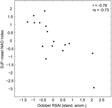
Figure 1. October Eurasian snow cover increase as described by the daily Robust Snow Advance Index (RSAI) plotted against the DJF-mean PC-based NAO. Displayed are the raw/non-detrended data as well as the Pearson (r) and Spearman (rs) correlation coefficients.
Download figure:
Standard image High-resolution imageThe relationship between the daily October RSAI and the DJF-mean W10 values is shown in figure 2(a). In case r is significant at a local test level of 5% (αlocal = 0.05), the corresponding grid box is marked with a white dot. A tripole of significant negative–positive–negative coefficients is found in the south-centre-north of the North Atlantic, yielding magnitudes of up to >0.8 (see figure 2(a)). Significant values are also found in the North Sea, the Baltic Sea and the western Mediterranean Sea. As shown in figure 2(c), the magnitude and pattern of r for SWH is similar to the results for W10, which was expected since the SWH at a given location is a function of local and remote wind forcing.
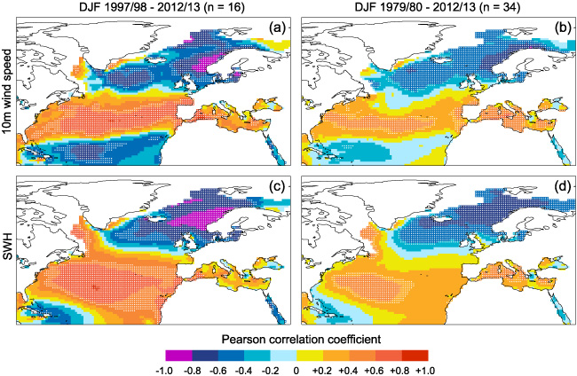
Figure 2. Pearson correlation coefficient between the October Robust Snow Advance Index (RSAI) and DJF-mean 10 m wind speed (W10) for using (a) the daily RSAI (n = 16) and (b) the weekly RSAI (n = 34). Significant correlation coefficients (α = 0.05, two-sided t-test, critical value for n − 3 degrees of freedom = ±0.51 and ±0.34 respectively) are marked by white dots. The corresponding results for DJF-mean significant wave height (SWH) are shown in panels (c) + (d). Results are based on linearly detrended predictor and predictand data.
Download figure:
Standard image High-resolution imageIn agreement with the results obtained for the large-scale circulation patterns, the strength of the statistical relationships decreases when using the degraded weekly RSAI over the long time period. Nevertheless, the spatial pattern is similar to that obtained from using the daily index over the short period and r remains significant over a large fraction of the study area (compare (b) + (d) to (a) + (c) in figure 2).
The corresponding results for (1) applying raw—instead of detrended data, (2) computing the Spearman—instead of the Pearson correlation and (3) using a modified t-test based on the effective sample size of the applied time series to calculate the p-values of r (Bretherton et al 1999, equation 31), are in close agreement to the results mentioned above (see S01, S02 and S03 in supplementary material available at stacks.iop.org/ERL/9/045006/mmedia). This indicates that the statistical relationships are generally insensitive to (1) removing or keeping the trend, (2) the presence of outliers and (3) the presence of serial correlation.
4. Statistical prediction
Based on the statistical relationships presented above, ordinary linear regression is used as a statistical prediction technique to hindcast the DJF-mean predictand values at each grid box from the October RSAI. For the short time period and the daily RSAI (1997/98–2012/13 n = 16), a one-year-out cross-validation approach is applied. Before hindcasting the ith withheld predictand value, the linear trend and the climatological mean are calculated on n − 1 values and are then removed from all data points. Note that n − 1 instead of n values are used for this purpose in order to avoid artificial skill; the withheld value and any information related to it is assumed to be unknown (von Storch and Zwiers 1999, Wilks 2006). To keep consistency, this procedure is also applied to the predictor variable.
The Pearson correlation coefficient between the hindcasted and observed DJF-mean values, hereafter referred to as 'hindcast correlation' (rhind), is displayed in the left column of figure 3. Only significantly positive hindcast correlations are displayed (α = 0.05, one-sided t-test, critical value = +0.44 for n − 3 degrees of freedom). In addition, the Root Mean Squared Error skill Score (RMSESS) is applied as alternative skill measure (see right column of figure 3). To calculate the RMSESS, the climatology of the detrended DJF-mean values (which is also calculated separately in each step of the cross-validation) is used as 'no skill' estimate. Hence, the RMSESS measures the percentage with which the climatological hindcast is outperformed by predicting with the October RSAI.
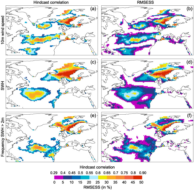
Figure 3. Hindcast skill obtained from the daily RSAI using 1-year-out cross-validation over the time period 1997/98–2012/13, n = 16. First column: significantly positive hindcast correlations (α = 0.05, one-sided t-test, critical value for n − 3 degrees of freedom = +0.44). Second column: positive root mean square error skill scores with reference to climatology (RMSESS). Results are for DJF-mean 10 m wind speed (a + b), DJF-mean significant wave height (c + d) and DJF-frequency of SWH > 2 m (e + f). Hindcasts are based on linearly detrended predictor and predictand data.
Download figure:
Standard image High-resolution imageAs can be seen from figure 3, the magnitude and pattern of skill is similar for the 3 variables under study. With rhind > 0.85 and RMSESS > 45%, skill is largest in the Norwegian Sea and the northern North Sea, and considerable skill is also obtained in the subtropical North Atlantic, the Baltic Sea and the western Mediterranean Sea. As an illustrative example for a possible practical application, figure 4 displays the results for SWH2m at the world's largest oil platform 'Troll A', located off the coast of southern Norway (60.65°N, 3.73°E). In this case, the hindcast is applied for the grid box nearest to the platform's location, using raw data which are more relevant in practice than detrended data. For this specific application, values of 0.89 and 55% are obtained for rhind and RMSESS respectively.
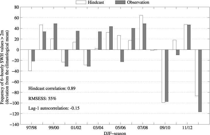
Figure 4. Hindcast skill for the DJF-frequency of SWH > 2 m at the ERA-Interim grid box nearest to the world's largest oil platform 'Troll A', located off the coast of southern Norway. Skill values and the lag-1 autocorrelation coefficient of the predictand variable are displayed in the lower left corner. Hindcasts are based on raw/non-detrended data.
Download figure:
Standard image High-resolution imageImportantly, positive serial correlation in the applied predictand time series may artificially enhance the hindcast skill estimates obtained from 1-year-out cross-validation. In this context, Michaelsen (1987) defines a lag-1 autocorrelation coefficient (acf1) > +0.25 as threshold value above which this problem becomes serious. For the variables applied here, the areal fraction of significant rhind and acf1 > +0.25 is below 2% in any case. It is therefore reasonable to assume that the results are not seriously affected by serial correlation.
To assess the robustness of skill over a longer time period, the statistical prediction scheme is also applied for the time period 1979/80–2012/13 (n = 34), using the degraded weekly RSAI for hindcasting. Since the sample size is larger in this case, an alternative cross-validation approach is used which further reduces the problem of serial correlation. Namely, the ith value to be predicted, together with the values of the previous and following 2 years (if available), are withheld in each step of the cross-validation. For ease of understanding, this approach will hereafter be referred to as '5-year-out cross-validation'. Figure 5 shows the respective results. If compared to figure 3, the magnitude of skill systematically decreases. Nevertheless, significant rhind (critical value = +0.29 for n − 3 degrees of freedom) and positive RMSESS are yielded in the above mentioned regions, excluding the central-subtropical Atlantic. The respective results for the non-detrended data and the short (long) time period are in close (broad) agreement (see figure S04 in the supplementary material available at stacks.iop.org/ERL/9/045006/mmedia). In addition, a split-sample test was conducted, using the period 1997/98–2012/13 for obtaining the forecast equation and the period 1979/80–1996/97 for testing the corresponding hindcasts with independent data. Prior to hindcasting, the mean value and the linear trend of the training sample were subtracted from the whole sample (this is done for both the predictor and the predictand), as was the case for cross-validation. As can be seen from figure S05 in the supplementary material (available at stacks.iop.org/ERL/9/045006/mmedia), the results for the split-sample test are in general agreement with those obtained from cross-validation. These sensitivity tests indicate that the hindcast results are generally robust to (1) applying a degraded snow index, (2) extending the study period, (3) using alternative verification procedures and (4) keeping or removing the trend.

Figure 5. As figure 3, but for the weekly RSAI using 5-year-out cross-validation over the time period 1979/80–2012/13, n = 34, critical value for n − 3 degrees of freedom = +0.29.
Download figure:
Standard image High-resolution image
5. Monte-Carlo field significance tests
Since the three hindcast approaches are repeated separately for each grid box of ERA-Interim (i.e. thousands of times), significant rhind are expected to occur at a number of grid boxes simply by chance. Hence, a Monte-Carlo field significance test is applied (Livezey and Chen 1983). The global null hypothesis (H0global) to be tested is: 'The areal fraction of significant hindcast skill obtained from the RSAI is due to chance'. To generate the corresponding null distribution, the three hindcast approaches described above (leave-1-out and leave-5-out cross-validation, split-sample test) are repeated 500 times using a randomly reshuffled RSAI in each repetition. The 95th percentile of the thereby obtained 500 areal fractions of significant rhind (arising from chance) is the critical value above which the H0global is rejected at a global test level of 5% (αglobal = 0.05). Note that this approach takes into account the spatial autocorrelation of the predictands. The corresponding results are displayed in table 2. The critical value is exceeded in any case, indicating that the H0global can be rejected with a 5% probability of error for any predictand variable and test configuration.
Table 2. Areal fraction of ERA-Interim grid boxes (in %) with locally significant (αlocal = 0.05) hindcast correlations obtained from cross-validation. Column 1: predictand variable. Column 2: fractions obtained from predicting with the daily RSAI over the short period (1997/98–2012/13, n = 16), using 1-year-out cross-validation. Column 3: fractions obtained from predicting with the weekly RSAI over the long period (1979/80–2012/13, n = 34), using 5-year-out cross-validation. Column 4: as column 3, but using a split-sample test (training period: 1997/98–2012/13, test period: 1979/80–1996/97). In each cell, the fraction obtained from using the right temporal order of the RSAI (first number) is compared to the 95th percentile of the 500 fractions obtained from randomly reshuffling the RSAI (second number, in brackets). Hindcasts are based on linearly detrended predictor and predictand data. Local p-values are calculated on n − 3 degrees of freedom.
| Predictand | Daily RSAI, leave-1-out | Weekly RSAI, leave-5-out | Weekly RSAI, split-sample |
|---|---|---|---|
| 10 m wind speed | 34(14) | 32(15) | 26(16) |
| SWH | 35(15) | 29(17) | 23(20) |
| SWH > 2 m | 29(11) | 18(10) | 17(15) |
6. Discussion and conclusions
The present study has proposed a statistical technique for forecasting DJF-mean wind and wave conditions in the North Atlantic from Eurasian snow cover increase in October as described by the Robust Snow Advance Index (RSAI). Applying cross-validation and split-sample tests for two distinct snow cover datasets, a short one based on daily- and a long one based on weekly snow cover values, the method yields significant hindcast skill for the northeastern North Atlantic, the North- and Baltic Seas and the western Mediterranean Sea. As indicated by Monte-Carlo field significance tests, it is very unlikely that these skill patterns arise from chance. However, the results are based on relatively small samples and consequently should be reconfirmed in the future.
Using degraded data to obtain a longer time series of the RSAI, hindcast skill systematically decreases but yet remains significant over a large fraction of the study area. This skill drop, which was also found in Brands et al (2012) for the case of wintertime precipitation, may be explained by the following arguments. First, for the common 16-year period of October 1997–2012, the weekly/degraded RSAI has been shown to perform worse than the daily one (compare column 2 to column 3 in table 1), indicating that it also likely underestimates the strength of the proposed teleconnection over the long period. Second, the large skill estimates obtained from the daily RSAI might arise from sampling uncertainty due to limited sample size (n = 16). Third, the strength of the snow–AO relationship is known to be non-stationary, i.e. varies along the course of the 20th century (Peings et al 2013), and a similar behaviour should be expected for the relationships presented here. A definite explanation for the 'skill drop' mentioned above can only be given in the future, when a larger time series of daily satellite-sensed snow cover becomes available.
It is important to note that the proposed statistical forecasting method by no means is intended to replace seasonal forecasts based on fully coupled general circulation models, since it relies on a single predictor variable and does not take into account possible non-linear relationships (Hsieh and Tang 1998). Furthermore, due to the stationarity issue mentioned above, skill inferred from past observations may overestimate real forecast skill (DelSole and Shukla 2009). Also, the study relies on reanalysis data which are often assumed to provide reliable seasonal-mean values (Semedo et al 2011, Le Cozannet et al 2011, Stopa et al 2013). Nevertheless, the results should ideally be reconfirmed with buoy data (Reguero et al 2012) or, if these are not available, with regional climate model output (Jerez et al 2013, Menendez et al 2013).
Having in mind these limitations, the proposed method might nevertheless serve as an additional tool for making seasonal forecast decisions, especially when taking account the limited skill of alternative approaches. As such, it is expected to be of interest for seafaring, fishery, coastal engineering, offshore oil drilling and power generation in the North Atlantic Ocean and adjacent seas.
Acknowledgments
This study was funded by the CSIC JAE-PREDOC programme, the EU FP7 projects SPECS (308378) and EUPORIAS (308291). The ECMWF ERA-Interim data (www.ecmwf.int/research/era/do/get/era-interim), the PC-based NAO index provided by James Hurrell (https://climatedataguide.ucar.edu/sites/default/files/climate_index_files/nao_pc_djf.txt), the EA and SCAND indices provided by the Climate Prediction Center (www.cpc.ncep.noaa.gov/data/teledoc), the IMS Daily Northern Hemisphere Snow and Ice Analysis at 24 km Resolution provided by the NSIDC (ftp://sidads.colorado.edu/pub/DATASETS/NOAA/G02156/24km/) and the weekly snow cover data provided by the Rutgers University Global Snow Lab (ftp://data.ncdc.noaa.gov/cdr/snowcover/) are acknowledged. The author is grateful to Dr José Manuel Gutiérrez and Dr Juan J Taboada for discussing the manuscript and to 4 referees for their helpful comments.