
Abstract
The extensive deforestation and degradation of tropical forests is a significant contributor to the loss of biodiversity and to global warming. Restoration could potentially mitigate the impacts of deforestation, yet knowledge on how to efficiently allocate funding for restoration is still in its infancy. We systematically prioritize investments in restoration in the tropical landscape of East Kalimantan, Indonesia, and through this application demonstrate the capacity to account for a diverse suite of restoration techniques and forests of varying condition. To achieve this we develop a map of forest degradation for the region, characterized on the basis of aboveground biomass and differentiated by broad forest types. We estimate the costs of restoration as well as the benefits in terms of carbon sequestration and improving the suitability of habitat for threatened mammals through time. When the objective is solely to enhance carbon stocks, then restoration of highly degraded lowland forest is the most cost-effective activity. However, if the objective is to improve the habitat of threatened species, multiple forest types should be restored and this reduces the accumulated carbon by up to 24%. Our analysis framework provides a transparent method for prioritizing where and how restoration should occur in heterogeneous landscapes in order to maximize the benefits for carbon and biodiversity.
Export citation and abstract BibTeX RIS

Content from this work may be used under the terms of the Creative Commons Attribution 3.0 licence. Any further distribution of this work must maintain attribution to the author(s) and the title of the work, journal citation and DOI.
Introduction
Deforestation and forest degradation are among the major drivers of biodiversity loss and carbon emissions in the tropics (Sodhi et al 2004, Harris et al 2012). Despite the rate of tropical deforestation declining in the 1990s (Achard et al 2002, DeFries et al 2002), this trend has since reversed, with an increasing rate of annual forest loss in some countries, notably Indonesia (Hansen et al 2013). While forest degradation has a broad definition, it is often associated with a reduction in forest biomass (Sasaki and Putz 2009, Sasaki et al 2011, Thompson et al 2013). Forest degradation is extensive, totalling 500–600 million hectares (or 30–40%) of the forest area in the tropics (Blaser et al 2011). In Indonesia alone, 82.9 million hectares (equating to 63.1%) of the Forest Estate that is under the authority of the Indonesian Ministry of Forestry is either degraded or deforested (Ministry of Forestry 2013a). Approximately 20 million hectares of this degraded forest is considered idle without a concession and hence targeted for illegal logging, land grabbing or gazetted for the development of oil palm plantations (Boer 2012, Levang et al 2012, Carlson et al 2013, Gaveau et al 2013).
Indonesia, and other tropical countries, could obtain funding to restore their forests through payments for ecosystem services under a variety of programmes including REDD+ projects (Reducing Emissions from Deforestation and forest Degradation) (UNFCCC 2007). Globally, the REDD+ program has generated carbon investments of up to US$2 billion since 2009 (Peters-Stanley et al 2013, Forest Trends 2014), in addition to a US$1 billion climate agreement between Norway and Indonesia (Solheim and Natalegawa 2010). Forest restoration is potentially more advantageous than other mechanisms (e.g. a focus on avoided deforestation alone) as it can engage and employ local people to undertake and maintain plantings (Alexander et al 2011). There is also a long history of experience with forest rehabilitation initiatives in Indonesia conducted by the government and non-governmental organizations, local communities, and the private sector, which could inform the implementation of restoration programmes (Nawir et al 2007, Barr and Sayer 2012).
The available funding and institutional resources however is unlikely to be sufficient to restore all degraded forest and priority must be given to particular areas (Nawir et al 2007, Boer 2012, Brockhaus et al 2012). The selection of areas to restore is complicated by variation in the capacity of forest types to sequester and store carbon due to inherent ecological characteristics, influenced also by climatic and edaphic gradients (Slik et al 2010, Budiharta et al 2014) and external pressures (e.g. logging, fire, and smallholder agriculture) (de Jong et al 2001, Langner et al 2007, Gaveau et al 2013). These interacting processes result in a broad spectrum of forest condition states, ranging from completely deforested to old-growth forest with minimal disturbance (Sasaki et al 2011, Thompson et al 2013). The condition of forests also influences the suitability of habitat for wildlife with some highly sensitive species requiring pristine forest while other species being more adaptable and able to persist in degraded forest (Meijaard et al 2005, Ansell et al 2011).
Forests of varying condition necessitates the consideration of a diverse suite of restoration techniques (Mori 2001, Sasaki et al 2011) which incur different costs associated with implementation and lost opportunities, including the costs associated with foregone profits of alternative land use or management (Lamb et al 2005, Wilson et al 2011a). For example, restoring a completely deforested site, such as an Imperata cylindrica grassland, would involve intensive planting with high implementation cost (Otsamo et al 1996), but the opportunity cost for the logging industry would be low due to a limited volume of harvestable timber remaining. Conversely, some degraded sites with considerable extant vegetation cover would require only enrichment planting, such as gap planting and strip planting, requiring a lower implementation cost (Korpelainen et al 1995, Maswar et al 2001, Soekotjo 2009). Restoration in this later case would likely forgo the potential revenues from harvesting remaining timber and thereby incur a higher opportunity cost (van Gardingen et al 2003, Ruslandi et al 2011).
Each restoration technique has a different contribution to forest growth, with the amount of accumulated carbon in the form of living biomass being related to planting density and design, often in a nonlinear way (Korpelainen et al 1995, Maswar et al 2001). The sequestration rates following planting also change through time. For instance, forest growth from strip plantings in a logged dipterocarp lowland forest in Borneo, follow a sigmoid curve with rapid carbon sequestration during the first 30 years (Hardiansyah 2011). Incorporating the time-dependent relationship of carbon sequestration and the costs associated with restoration allows the cost efficiency of each restoration action through time to be determined (Wilson et al 2011b). The cost efficiency of restoration is particularly relevant due to the finite amount of funding available for restoration programmes (Nawir et al 2007, Barr et al 2010, Peters-Stanley et al 2013).
Only a handful studies concerning the systematic prioritization of restoration on degraded tropical forests address the heterogeneity of these landscapes but have not explicitly accounted for carbon accumulation as a restoration objective (e.g. Marjokorpi and Otsamo 2006, Goldstein et al 2008). While more recent studies investigate restoration within the framework of carbon sequestration, they do not utilize systematic decision theoretic approaches (e.g. Sasaki et al 2011, Gilroy et al 2014). Analyses focussed on prioritising restoration for carbon sequestration have been in the context of cleared agricultural lands in non-tropical regions (e.g. Crossman et al 2011, Renwick et al 2014) and have focussed on only a single restoration technique (i.e. high density planting). The trade-off between carbon sequestration and biodiversity goals also warrants investigation given emerging initiatives to restore the habitat of threatened species (e.g. the Indonesian Orangutan Habitat Restoration Project) and degraded ecosystems (e.g. Katingan Peat Forest Restoration Project) (Rahmawati 2013, Starling Resources 2014). It is therefore timely to investigate restoration prioritisation approaches that can facilitate the identification of solutions for restoration that aim to satisfy the dual objectives of carbon sequestration and biodiversity conservation.
Here, we develop and apply a new framework for prioritising restoration that accounts not only for deforested areas, but also forest with varying condition. The framework is applied to East Kalimantan, Indonesia, to inform REDD+ policy implementation and conservation initiatives in the region. It provides the first assessment of the extent of degraded forests in East Kalimantan and their distribution across forest types. Alternative objectives for restoration are explored and trade-offs between carbon sequestration and improving the suitability of habitat for threatened mammals investigated. Finally, we provide recommendations of where and how restoration should be implemented in order to maximise the accumulation of carbon and improve the habitat for threatened species.
Methods
Study area
East Kalimantan is an Indonesian province of the island of Borneo (figure 1). East Kalimantan, and Borneo in general, is of global importance for both carbon storage and biodiversity. The aboveground biomass (AGB) carrying capacity per unit area of Bornean forests is 60% higher than Amazonian forests (Slik et al 2010). Borneo is also the major evolutionary source of biodiversity in Southeast Asia, resulting in extremely high species richness (de Bruyn et al 2014). Despite their vital role in the global carbon cycle and biodiversity conservation, the combination of logging, oil palm development, mineral extraction, and forest fires threatens biodiversity of the region and is the primary source of carbon dioxide emissions for the region (Carlson et al 2013, Pearson et al 2014, Budiharta and Meijaard in press).
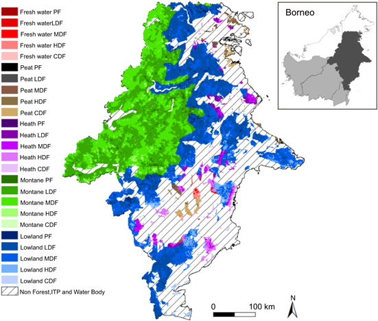
Figure 1. Map of forest condition across forest types in East Kalimantan. The study area is restricted to the Forest Estate with native vegetation under the authority of the Ministry of Forestry and excluded areas of Non-forest Estate, ITP (industrial timber plantation), mangroves, and water bodies.
Download figure:
Standard image High-resolution image
Jurisdictionally, land use in East Kalimantan is categorized into two classes: Forest Estate (Kawasan Hutan/KH) and Non-forest Estate (Area Penggunaan Lain/APL). Forest Estate, either forested or deforested, is defined as land use designated by the government to be permanent forest and under authority of the Ministry of Forestry (MoF; e.g. production forest (including industrial timber plantation (ITP)), protection forest and national park). Non-forest Estate is land outside the Forest Estate and includes both forested lands (e.g. private forest/forest garden) and non-forested lands (e.g. settled areas, road network and agricultural lands). We are interested in forest landscape restoration using native species and therefore focus only on the Forest Estate that has native vegetation cover. Therefore, we exclude the Non-forest Estate and Forest Estate allocated for ITP, which primarily uses single exotic species (e.g. Acacia mangium). Within this part of the Forest Estate, which is delineated based on Provincial Spatial Planning and Forest Land Use by Consensus (Ministry of Forestry 2011, 2012a), we create a planning unit layer by dividing the study area into pixels with a resolution of 400 hectares. This resolution represents a compromise to reduce computational time, capture environmental variability, and informative for policy and management implementation given the overall extent of the study region. Our study area covers 12.3 million hectares (63.2%) of the total land area of East Kalimantan (figure 1). All spatial analyses are conducted using ArcMap version 10.2 (ESRI 2013).
Analysis framework
We use a decision-support tool, Robust Offsetting (RobOff) (Pouzols and Moilanen 2013). RobOff is a resource allocation algorithm to prioritize 'how much' of an alternative management option should be allocated to 'which' environment. The objective is to maximize the benefit to features (e.g. species) given a particular level of investment considering the different response of features to management action across environments through time (Pouzols and Moilanen 2013). The algorithm can account for multiple environments and multiple management actions.
RobOff requires the environments being analysed to be characterized. These environments are an aggregation of planning units that share similar characteristics, such as land uses, land cover, forest types, and management activities. For our analysis, we define environments as a combination of forest types and degradation levels and herein refer to them as zones. Information on the characteristics of each zone is required including the proposed restoration action(s) and cost(s) of implementing these, the available area for undertaking each action, the occurrence of features (as a binary presence or absence), and the response of each feature to the action (measured on an annual basis). We focus on carbon and biodiversity as our features of interest, and employ AGB (in tonnes) accumulation and the suitability of habitat for threatened mammals as surrogates for these features. Among the taxonomic groups that occur in the region, mammals have the best available data and are the most prominent in conservation policy (Soehartono et al 2008).
Within the RobOff framework, we explore alternative scenarios representing four objectives: (1) prioritize carbon benefit by maximizing AGB accumulation, (2) prioritize biodiversity benefit by maximizing the improvement of habitat for threatened mammals, (3) prioritize both AGB accumulation and improvement of habitat for threatened mammals, and (4) prioritize forest types that are highly degraded. We run the algorithm over a 30 year planning horizon and employ a 6.5% discount rate in calculating costs (Bank Indonesia 2013).
Restoration zones
We develop a stratification matrix of forest condition for East Kalimantan based on the level of degradation and apply this across broad forest types following Gibbs et al (2007). In East Kalimantan, logging and fire have been the main drivers of forest degradation with obvious impacts on the reduction of AGB (Langner et al 2007, Gaveau et al 2014, Pearson et al 2014). We therefore use the extant stock of AGB as a proxy for the level of degradation, assuming that the highest value of AGB observed for a forest type is representative of an intact/pristine condition (table 1) (Mori 2001, Sasaki et al 2011). We obtain estimates of AGB from LiDAR calibrated with 4079 field measured plots (Saatchi et al 2011). The Saatchi AGB map has a 1 km spatial resolution, and among available carbon maps, it has the best agreement with the plot inventory data for Bornean rainforest collated by Slik et al (2010). We assign six broad forest types using ecoregion data (Olson et al 2001, Wikramanayake et al 2002) to deliver six forest types across East Kalimantan. Mangrove forest is excluded from our analysis as it represents a transitional ecosystem between terrestrial and marine biomes, complicating the specification of soil parameters in the AGB modelling (see below). We identify 25 restoration zones representing a combination of five degradation levels and five forest types (table 1, figure 1).
Table 1. Restoration zones in East Kalimantan based on a forest condition matrix across five forest types. The five condition classes are critically degraded/deforested (CDF), highly degraded (HDF), moderately degraded (MDF), lightly degraded (LDF), and primary forest (PF). The highest value of AGB observed for each forest type was assumed to represent intact/pristine forest, with the condition classes assigned in relation to this baseline such that CDF = ≤ 20%; HDF = 21%–40%; MDF = 41%–60%; LDF = 61%–80%; and PF = >81%. AGB stock is in Mg ha−1.
| Forest type | Primary forest | Lightly degraded | Moderately degraded | Highly degraded | Critically degraded |
|---|---|---|---|---|---|
| Lowland forest | ≥ 411 | 308–410 | 206–307 | 103–205 | ≤ 102 |
| Montane forest | ≥ 374 | 280–373 | 187–279 | 94–186 | ≤ 93 |
| Heath forest | ≥ 351 | 263–350 | 176–262 | 88–175 | ≤ 87 |
| Peat swamp forest | ≥ 345 | 260–345 | 173–259 | 87–172 | ≤ 86 |
| Freshwater swamp forest | ≥ 213 | 160–212 | 107–159 | 54–106 | ≤ 53 |
Restoration actions and costs
We determine the plausible restoration action for each restoration zone based on the published literature and government regulations (Korpelainen et al 1995, Maswar et al 2001, Mori 2001, Lamb et al 2005, Wibisono et al 2005, Hardiansyah 2011, Sasaki et al 2011, Ministry of Forestry 2012b, 2013b) (table 2, and S1 in the supplementary data available at stacks.iop.org/ERL/9/114020/mmedia). Specifically, the focus is on active restoration, assuming plantings of native tree seedlings of species predominately from the Dipterocarpaceae family at three degradation levels: critically, highly and moderately degraded forest (table 2) and passive restoration (i.e. natural regrowth) on primary or lightly degraded forest is not accounted for.
Table 2. Restoration actions and costs (in US$/hectare) across restoration zones. Restoration costs consist of the implementation costs of planting (table S1) and the revenue foregone from timber extraction.
| Restoration zones | Actions | Cost (US$/hectare) |
|---|---|---|
| Lowland CDF | Intensive square planting | 1275 |
| Lowland HDF | Strip planting | 943 |
| Lowland MDF | Gap planting | 1395 |
| Montane CDF | Intensive square planting | 1450 |
| Montane HDF | Strip planting | 1024 |
| Montane MDF | Gap planting | 1435 |
| Heath CDF | Intensive square planting | 1964 |
| Heath HDF | Strip planting | 1231 |
| Heath MDF | Gap planting | 1539 |
| Peat swamp CDF | Intensive square planting | 1518 |
| Peat swamp HDF | Strip planting | 1047 |
| Peat swamp MDF | Gap planting | 1447 |
| Freshwater swamp CDF | Intensive square planting | 1463 |
| Freshwater swamp HDF | Strip planting | 1025 |
| Freshwater swamp MDF | Gap planting | 1435 |
Cost is divided into two categories: implementation and opportunity cost. Implementation costs consist of expenditure for planting and maintenance. We use the standard cost of planting prescribed by the Indonesian government (Ministry of Forestry 2012b) as a baseline with additional maintenance costs (e.g. fire control and patrolling activities) up to the fourth year as suggested by Hardiansyah (2011). These data are employed for lowland forest with modifiers based on literature review and personal communications with restoration practitioners to obtain implementation costs for the remaining forest types (table S1). For example, preparing planting sites on peat swamp forests would require the construction of artificial mounds to minimize seedling mortality due to prolonged flooding (Wibisono et al 2005). This activity would incur an additional cost of US$77 per hectare when restoring critically degraded peat swamp forest. We also explore the sensitivity of our results to the potential additional cost required for hydrological restoration in peat swamp forest using data from Ex-Mega Rice Peatland Rehabilitation Project in Central Kalimantan (KFCP 2009). As the costs vary depending on the type of dam constructed and material used, we use an average cost of US$278 per hectare.
We define the opportunity cost of forest restoration as the revenue foregone from timber extraction as a consequence of restoration. The average net present value (NPV) of timber harvesting in intact forest in Kalimantan (i.e. US$2,268 per hectare) is employed as a baseline for this cost type (Ruslandi et al 2011). For moderately degraded forest, harvestable timber is reduced by approximately 40% (following van Gardingen et al 2003), resulting in a NPV of US$ 975.24 per hectare. For highly degraded forest, most of the trees are below the diameter cutting limit and large-scale commercial logging operations are no longer profitable (Sasaki et al 2011). A conservative value of US$300 per hectare is therefore assigned as the opportunity cost for timber harvesting in these areas. For critically degraded forest, we do not assign an opportunity cost for timber harvesting as most remaining trees are pioneer species (Macaranga spp.) and commercial dipterocarp species are rare and small in size (Mori 2001).
Restoration investment
We employ a theoretical budget of US$500 million. We increase the budget by 2.5 times to explore the influence of budget availability on the zones prioritized for restoration and on the trade-offs observed between carbon and biodiversity.
Estimating AGB accumulation
The response of AGB when restoring each zone is estimated using a process-based model called 3-PG (physiological principles for predicting growth). Despite the initial purpose to predict the growth of monoculture plantations in temperate regions (Landsberg and Sands 2011), this model has also performed well for estimating AGB of highly diverse forests in the tropics (White et al 2006, Budihartaet al 2014). The model requires soil and climate variables as inputs, along with a set of physiological parameters.
We obtain soil texture classes, fertility ratings and maximum and minimum plant available soil water estimates from the Harmonized World Soil Database (FAO/IIASA/ISRIC/ISSCAS/JRC 2012). Climate input variables, including monthly temperature (i.e. maximum, mean and minimum), monthly precipitation and vapour pressure deficit, were obtained from the WorldClim database (Hijmans et al 2005) and solar radiation estimated from the monthly averages of surface insolation from 22 years of satellite observation provided by the POWER project (The Prediction of Worldwide Energy Resource) (NASA 2013). We employ physiological parameters developed specifically for Bornean rainforest and differentiated by forest type (Budihartaet al 2014). We estimate AGB accumulation over 30 years for each degradation level for each forest type (i.e. each restoration zone). In each zone, we assume that AGB is accumulated from two sources: natural regrowth of existing vegetation and restoration planting in a specific design depending on the level of degradation (table 2). Therefore, we separately model the AGB accumulated from both processes, then combine the results to estimate the total AGB accumulated for each restoration zone.
Estimating the suitability of habitat for threatened mammals
Our analysis focuses on threatened mammal species within the IUCN classes vulnerable and above (27 vulnerable species and ten endangered species) (IUCN 2013). To reduce uncertainty in species distributions, we intersect the habitat suitability models of terrestrial mammals (Rondinini et al 2011) with their known geographical extent (IUCN 2013). The resultant map is then overlaid with the restoration zones to determine the possible occurrence of each mammal in each zone. In total, 35 threatened mammal species occur within the zones being considered for restoration (table S2).
We assume that the relationship between the suitability of habitat for each species and the extent of forest cover is determined by the sensitivity of each species to forest degradation (Wilson et al 2010) and the habitat suitability would change overtime as forest restored. The sensitivity level was assessed by expert elicitation complemented with literature review, and classified into three classes: low, medium and high sensitivity (Wilson et al 2010). Forest cover derived from moderate resolution imaging spectroradiometer (MODIS) (Townshend et al 2011) was related to the AGB derived from Saatchi et al (2011). We used R Statistical Software (R v. 3.0.1 R Development Core Team 2013) for the regression analysis and the resultant relationships were significant at the level of P < 0.001 (table S3). We then employed the relationship per forest type to derive the habitat suitability of threatened mammals.
Habitat suitability is estimated for each species within each restoration zone over 30 years using the following arbitrary rules: (i) for highly sensitive mammals nearly complete (90%) forest cover is required; (ii) for moderately sensitive species the majority (60%) of forest cover is required; and (iii) for low sensitivity species then only a small proportion (30%) of forest cover is required. We explore the sensitivity of our results by decreasing and increasing the baseline threshold of forest cover suitable for each mammal sensitivity class by 10%.
Results
We estimate that 6.1 million hectares (49.6%) of Forest Estate land (excluding ITP) in East Kalimantan is in critically, highly or moderately degraded condition, requiring active restoration (table 3). Degradation is not uniformly distributed across forest types with peat swamp forest having the largest proportion of degraded areas (93.7%) followed by freshwater swamp forest (92.9%), while montane forest has the lowest (46.3%). The total budget needed to restore all degraded forests identified would be approximately US$8.37 billion if we consider both the implementation and opportunity costs, and US$3.24 billion if we only account for the implementation cost.
Table 3. Summary of degradation levels across forest types: total extent (thousands of hectares) and the proportion of the overall extent of this forest type.
| Forest types | ||||||
|---|---|---|---|---|---|---|
| Degradation classes | Lowland | Montane | Heath | Peat swamp | Freshwater swamp | Total |
| Primary and lightly degraded | 2994 (53%) | 3029 (53.7%) | 171 (25%) | 17 (6.3%) | 4 (7.1%) | 6217 |
| Moderately degraded | 2178 (38.6%) | 2467 (43.7%) | 258 (37.8%) | 65 (23.6%) | 13 (21.9%) | 4984 |
| Highly degraded | 428 (7.6%) | 145 (2.6%) | 206 (30.2%) | 70 (25.3%) | 36 (57.6%) | 887 |
| Critically degraded | 44 (0.8%) | 1 (0.0%) | 48 (7%) | 124 (44.8%) | 8 (13.4%) | 227 |
| Total | 5646 | 5644 | 683 | 278 | 63 | 12 316 |
Regardless of the objective and budget, it is recommended that highly degraded lowland forest be extensively restored (tables 4 and 5). Restoring this zone incurs the lowest restoration costs, contributes to the restoration of the habitat of 29 of 35 threatened mammals, and accumulates the greatest amount of AGB. Heath forest has the smallest area recommended for restoration, with the exception of when the goal is to recover forest types that have been extensively degraded (scenario 4). The implementation cost of planting heath forest is the highest of all forest types, while the accumulation of AGB is relatively low due to infertile soil (table S1). Regardless of forest type, moderately degraded forest is least favoured for restoration (table 4), due to the presence of large commercial trees, which incurs a very high opportunity cost.
Table 4. Recommended areas for restoration under each scenario using the lower investment level (US$500 million).
| Restoration zones | Available area (ha) | Scenario 1 (ha) | Scenario 2 (ha) | Scenario 3 (ha) | Scenario 4 (ha) |
|---|---|---|---|---|---|
| Lowland CDF | 44 127 | 0 | 0 | 0 | 44 127 |
| Lowland HDF | 428 645 | 428 645 | 164 238 | 428 645 | 52 042 |
| Lowland MDF | 2178 922 | 0 | 3582 | 0 | 0 |
| Montane CDF | 1776 | 0 | 0 | 1776 | 1776 |
| Montane HDF | 145 760 | 93 045 | 145 760 | 10 508 | 0 |
| Montane MDF | 2467 541 | 0 | 0 | 0 | 0 |
| Heath CDF | 48 057 | 0 | 0 | 0 | 48 057 |
| Heath HDF | 206 454 | 0 | 0 | 0 | 40 868 |
| Heath MDF | 258 400 | 0 | 0 | 0 | 0 |
| Peat swamp CDF | 124 894 | 0 | 124 894 | 0 | 0 |
| Peat swamp HDF | 70 584 | 0 | 0 | 70 584 | 70 584 |
| Peat swamp MDF | 65 744 | 0 | 0 | 0 | 65 744 |
| Freshwater swamp CDF | 8478 | 0 | 0 | 0 | 8478 |
| Freshwater swamp HDF | 36 401 | 0 | 0 | 4142 | 36 401 |
| Freshwater swamp MDF | 13 802 | 0 | 0 | 2271 | 13 802 |
| Total area (ha) | 6099 585 | 521 690 | 438 474 | 517 926 | 381 879 |
| Total budget (US $ million) | — | 499.86 | 498.94 | 499.25 | 491.25 |
| Total AGB (million tonnes) | — | 226.16 | 170.93 | 215.99 | 126.70 |
| Number of mammals occurring in prioritized restoration zones | — | 31 | 35 | 34 | 34 |
Table 5. Recommended areas for restoration with investment higher restoration budget (US$1,250 million).
| Restoration zones | Available area (ha) | Scenario 1 (ha) | Scenario 2 (ha) | Scenario 3 (ha) | Scenario 4 (ha) |
|---|---|---|---|---|---|
| Lowland CDF | 44 127 | 44 127 | 0 | 0 | 44 127 |
| Lowland HDF | 428 645 | 428 645 | 428 645 | 428 645 | 428 645 |
| Lowland MDF | 2178 922 | 454 704 | 387 873 | 429 635 | 0 |
| Montane CDF | 1776 | 1776 | 1776 | 1013 | 1776 |
| Montane HDF | 145 760 | 145 760 | 81 518 | 145 760 | 145 760 |
| Montane MDF | 2467 541 | 0 | 0 | 0 | 0 |
| Heath CDF | 48 057 | 0 | 535 | 0 | 48 057 |
| Heath HDF | 206 454 | 0 | 0 | 0 | 0 |
| Heath MDF | 258 400 | 0 | 0 | 0 | 80 185 |
| Peat swamp CDF | 124 894 | 0 | 124 894 | 0 | 34 392 |
| Peat swamp HDF | 70 584 | 0 | 0 | 70 584 | 70 584 |
| Peat swamp MDF | 65 744 | 0 | 0 | 0 | 65 744 |
| Freshwater swamp CDF | 8478 | 0 | 8478 | 8478 | 8478 |
| Freshwater swamp HDF | 36 401 | 0 | 10 318 | 3162 | 36 401 |
| Freshwater swamp MDF | 13 802 | 0 | 0 | 3773 | 13 802 |
| Total area (ha) | 6099 585 | 1075 012 | 1044 037 | 1091 050 | 977 951 |
| Total budget (US$ million) | — | 1247.41 | 1245.61 | 1249.95 | 1121.35 |
| Total AGB (million tonnes) | — | 462.28 | 431.44 | 456.60 | 373.38 |
| Number of mammals occurring in prioritized restoration zones | — | 32 | 35 | 35 | 35 |
If the lower restoration budget (US$500 million) is assumed and the objective is to prioritize AGB accumulation (scenario 1) the entire budget is allocated predominately to restoring highly degraded lowland and montane forest. This scenario achieves the best carbon outcome with 226 million tonnes of AGB stored over 30 years (table 4). The restoration of highly degraded lowland forest contributes 83% of the AGB predicted to be accumulated and consumes 81% of the total budget. However, this carbon outcome would be at the expense of biodiversity goals with the habitat of Bornean elephant (Elephas maximus borneensis) and aquatic mammals, including oriental small-clawed otter (Aonyx cinerea), hairy-nosed otter (Lutra sumatrana) and smooth-coated otter (Lutrogale perspicillata), not receiving any restoration investment (table S2).
The highest biodiversity benefit is achieved under scenario 2 (prioritizing the restoration of threatened mammal habitat) with the zones selected for restoration encompassing the distributions of all threatened mammals (table 4 and S2). This comes at a cost in terms of the total AGB accumulated which is reduced by 24.4% compared to that achieved under scenario 1. The overall extent of the area restored is also reduced by 16%. The restoration of the habitat of Bornean elephant is accommodated by selecting 3582 hectares of moderately degraded lowland forest. Within our restoration zones, Bornean elephants are restricted to a small area near the border with Sabah which overlaps with moderately degraded forest in lowland and montane forest. A large amount of the budget is also allocated to restoring the habitat of aquatic mammals with the selection of 124 894 hectares of critically degraded peat swamp forest as this zone harbours all aquatic threatened mammals.
Prioritizing both AGB accumulation and the restoration of threatened mammal habitat (scenario 3) would deliver a more balanced solution. Under this scenario, total AGB stored is only 4.5% lower than scenario 1 (prioritising AGB accumulation alone) with only Bornean elephant not receiving any investment (table 4 and S2). Prioritizing heavily degraded forest types (scenario 4) results in the investment fund being distributed across a greater diversity of restoration zones, regardless of the higher cost of restoration (table 4). As a consequence, this scenario performs worst in terms of carbon sequestration and biodiversity outcomes, with only 126 million tonnes of AGB stored and no restoration afforded to the habitat of Bornean elephant (table S2). Under this scenario, all available restoration zones within freshwater swamp are selected for restoration, while for peat swamp and heath forest, only 52% and 17.3% of the available areas are prioritized respectively. Only 98% of the available budget is used in scenario 4, indicating that the prioritization of heavily degraded forest types obtained the maximum possible outcome for this objective and continued allocation of funding would be counterproductive considering the very high costs incurred.
When the budget is increased (by 2.5 times), the trade-offs between objectives is reduced (table 5). If the restoration of threatened mammal habitat is the focus (scenario 2) then all mammals will obtain some investment and accumulation of AGB would be reduced by 6.7% compared to scenario 1 (prioritizing AGB accumulation). Conversely, under scenario 1, no investment would be allocated to restore the habitat of three aquatic mammals (table 5 and S2). Optimizing both carbon and biodiversity objectives (scenario 3) results in the habitat of all threatened mammals receiving investment with AGB accumulation only 1.2% lower than under scenario 1.
Our results are insensitive to the threshold of forest cover suitable for each mammal sensitivity class. Either by decreasing and increasing the baseline threshold by 10%, all available areas of highly degraded lowland forest are consistently prioritized when the objective is carbon accumulation (scenario 1) and dual objectives (scenario 3). In addition, when focusing on threatened mammals' habitat (scenario 2), a comparably large portion of investment is constantly allocated to highly degraded lowland and montane forests, and critically degraded peat swamp forest. Interestingly, adding a cost associated with hydrological restoration in peat swamp forest does not change the overall results, even for scenario 2 in which all areas of critically degraded peat swamp forest is prioritized for restoration. This is likely because of the unique conservation value of this zone due to the occurrence of all aquatic mammals.
Discussion
We present a novel framework for systematically prioritising restoration areas that explicitly accounts for the contribution of a variety of restoration actions and for the heterogeneous nature of landscapes. We characterize a broad spectrum of landscape conditions, assign plausible restoration actions, estimate costs and benefits for multiple actions, and adapt a newly developed decision support tool to prioritising the allocation of restoration investments.
By applying our framework in East Kalimantan, we find that highly degraded lowland forest (with 21%–40% AGB remaining) is favoured for restoration, particularly if the objective is to enhance carbon stocks. This is due to the comparatively low costs associated when restoring this zone and the rapid accumulation of AGB. Regardless of objective, a large portion of the budget is always allocated to restoring highly degraded lowland forest, highlighting the importance of this zone for both carbon sequestration and restoring the habitat of threatened mammals. Murdiyarso et al (2011) criticised the Indonesian government following the REDD+ agreement with Norway, which only protects primary forests and peat lands from new permits for logging concession and conversion and excludes 46.7 million hectares of logged and secondary forests. Our finding corroborates Murdiyarso and colleagues' proposal for the inclusion of degraded forests into the moratorium, particularly for over 400 000 hectares of highly degraded lowland forest in East Kalimantan. Apart from government funded REDD+ initiatives, our results suggest that these areas are the first priority for allocating Ecosystem Restoration Concession (Boer 2012). This new policy has attracted private investments to restore degraded forests either for carbon credit (e.g. Rimba Raya InfiniteEarth), biodiversity conservation (e.g. Harapan rainforest) or both (The Guardian 2013, Birdlife International 2014).
Moderately degraded forests (with 41%–60% AGB remaining) are recommended for restoration if budget is not limiting and the objective is to restore the habitat of threatened species (scenario 2). The considerable volume of remaining timber in moderately degraded forests incur a high opportunity cost, suggesting that forests under this degradation category are better managed for selective logging, provided they also occur on forests sanctioned for timber production (Hutan Produksi). Across Kalimantan, well managed logging concessions have maintained forest cover and delivered significant contributions to biodiversity conservation (Meijaard et al 2005, Wilson et al 2010, Gaveau et al 2013). Restoring critically degraded forests (with 0%–20% AGB remaining) is recommended only if a larger budget is available (table 5). An emerging option for restoration of these areas is to generate socio-economic benefits for local people, for example by the establishment of agroforestry under the legal framework of community forest (Hutan Kemasyarakatan) (Ministry of Forestry 2007), which can be funded by the ongoing national forest rehabilitation programme (i.e. Gerakan Nasional Rehabilitasi Lahan dan Hutan/GERHAN). In the worst conservation scenario, if the Forest Estate is converted to agriculture (e.g. oil palm plantation), targeting critically degraded forests for such conversion is a wise option, as also suggested by Koh and Ghazoul (2010).
We discover trade-offs between the objectives of carbon and biodiversity, but these are highly dependent upon the budget available. When the budget is limited, AGB accumulation under scenario 2 (prioritizing the restoration of threatened mammal habitat) would be 24.4% lower than scenario 1 (prioritizing AGB accumulation only). However, the AGB scenario would fail to restore four of 35 mammals' habitat. Under the higher budget, AGB accumulation under scenario 2 would only be 6.7% lower than scenario 1, with the habitat of an additional mammal receiving investment. Our finding reveals that with small adjustments, we could achieve a compromise solution for the dual objectives of carbon and biodiversity (scenario 3). Employing the lower budget, the accumulation of AGB under scenario 3 is only 4.5% lower than scenario 1 with one mammal not receiving habitat restoration. This more balanced solution was also found by Venter et al (2009) for the REDD+ activity of avoided deforestation, with the number of species protected doubled for a reduction of just 4%–8% in emissions avoided. In our case study, the trade-offs are influenced by species with either limited geographic range (such as Bornean elephant) or unique habitat requirements (such as oriental small-clawed otter, hairy-nosed otter and smooth-coated otter).
Although it might reduce the carbon benefit and increase opportunity costs, restoration for biodiversity objectives is likely to attract socio-political support and financial contributions from the public (Dinerstein et al 2013). For example, in 2012, Indonesian Orangutan Habitat Restoration Programme generated revenues amounting to US$6.4 million for managing three restoration and reintroduction projects in Kalimantan, increasing from US$4.0 million in 2011 (BOS Foundation 2013). Similar initiatives could be expanded to restore the habitat of Bornean elephant, as this species has a limited distribution in East Kalimantan and current protected areas do not afford adequate protection (Wilson et al 2010). Protection of this species will however incur high opportunity costs as its distribution overlaps with moderately degraded forests that are currently allocated for logging concessions (Gaveau et al 2013).
Our restoration framework does not account for passive restoration alone as this option is unlikely to be effective in the medium and long term. In highly degraded dipterocarp forest in Borneo, local recruitment of dipterocarp seedlings is limited because of seed predation and a lack of reproductively mature adults due to past harvesting (Ådjers et al 1995, Curran and Webb 2000). Recruitment through seed dispersal is low because dipterocarp seeds are heavy, poorly dispersed and recalcitrant which result in low germination success (Ådjers et al 1995, Kettle 2010). Further, the resilience of pioneer species (e.g. Macaranga stands) constrains the remaining dipterocarp seedlings from obtaining access to nutrients and sunlight, necessitating active management, such as strip planting, to enhance restoration success (Cannon et al 1994, Hardiansyah 2011, Aoyagi et al 2013). Apart from ecological constrains, Zahawi et al (2014) warn that passively restored sites are often regarded as abandoned land and open access, leading to perverse actions (e.g. land encroachment, fallow practices) and jeopardizing restoration goals. This situation could incur what they termed a 'hidden cost of passive restoration' and is likely more apparent in developing countries where land tenure is often unclear.
To our knowledge, comprehensive data representing forest degradation is not available for Borneo, or more specifically East Kalimantan, with the exception of spatial data of degraded lands (Lahan Kritis) released by the MoF (Ministry of Forestry 2011). This dataset broadly delineates the state of certain areas for supporting hydrology and soil protection (e.g. vulnerability to flooding and soil erosion) rather than detailed vegetation condition. While we mapped forest condition based on the remaining AGB within a forest type, maximum AGB for intact forest could vary among sites (Ziegler et al 2012) and therefore it would be preferred if the degradation threshold to be differentiated at a local scale. For selectively logged forests, logging techniques have varying intensity and diverse impacts on soil with some areas suffering extensive topsoil erosion and compaction, impeding vegetation recovery either through natural regrowth or enrichment planting (Pinard et al 2000). In peat swamp forest, degradation is often associated with modifications to drainage systems, and hydrological restoration through re-wetting and canal blocking can be required prior to vegetation restoration (KFCP 2009). The coarse resolution of the spatial data that we employ (particularly for forest types), along with the simplified, yet robust approach to stratify AGB warrants further field validation. In the future, integration of fine resolution estimates of extant biomass and vegetation cover as well as soil and hydrological condition would be beneficial to develop a more accurate assessment of forest degradation.
The suitability of habitat for threatened species was estimated through expert elicitation although our results are insensitive to the changes in the sensitivity thresholds. Wildlife exhibit specific responses to the dynamics of habitat resources following restoration, and the habitat suitability of particular species is often associated with elements in addition to canopy cover, such as tree hollows and the occurrence of vines and shrubs (Edwards et al 2009, Ansell et al 2011). Unfortunately, this kind of detailed information is unknown for most of mammals in East Kalimantan, except for well-known species such as Bornean orangutan. Further empirical analysis of the dynamic contribution of restored forest to habitat suitability is required to fill this knowledge gap. Spatial configuration also affects the habitat suitability of species in regard to the shape and connectivity of habitat patches with some mammals (e.g. Bornean elephant) requiring extensive and well-connected habitat (Alfred et al 2012). This problem is not addressed by RobOff as it does not produce spatially-explicit results. Further field based research is therefore required to determine the level of spatial cohesion and connectivity required for the species of interest. Ideally, the impact of climate change would be accounted for to estimate the suitability of habitat during the entire planning horizon. This analysis would require fine-resolution downscaling of environmental variables validated with long-term meso-and-fine scale climate data, which is presently unavailable for East Kalimantan.
We define opportunity cost as the potential revenue forgone from timber extraction as the consequence of restoration. There is however a risk for restored forest to be harvested, thereby reducing the opportunity cost. We could explore an additional scenario that accounts for the potential for profits to be generated from restored forests. While our study area is within the Forest Estate, which is designated for forestry and conservation purposes, it could be relevant to also explore the opportunity costs of alternative land-use options given the highly dynamic land-use changes in the region aimed at boosting the economy (Koh and Ghazoul 2010). In Kalimantan, oil palm plantation alone is predicted to triple in area extent by 2020 (Carlson et al 2013). However, this modification should also account the socio-political costs of changing land-use (e.g. lobbying officials, amending regulations, potential legal disputes, and potential conflicts with communities) which is problematic to determine due to low levels of governance and high levels of corruption in Indonesia (Faisal 2013).
While our analysis pioneers an approach for prudent and transparent allocation of restoration investments in heterogeneous landscapes from an ecological perspective, accounting for socio-political variables would also be vital for restoration planning and decision-making. Social perception of local communities in valuing the forest varies spatially across the landscapes, depending on how they utilize the goods and services provided (Abram et al 2014). As such, there will be communities that benefit and are disadvantaged by restoration, and the outcomes for communities may trade-off with ecological outcomes. To avoid perverse social impacts, some restoration projects could involve local people by recruiting them as labour (Birdlife International 2014), create incentive systems to ensure that the restored forests are protected and maintained (Limin et al 2008), and provide alternative livelihoods through better management of non-timber forest products (e.g. honey bees, rattan and medicinal plants) generated by the restored forests (Rahmawati 2013, Birdlife International 2014). In Indonesia, substantial improvement in governance would also be required, as these were the major cause of the failure of previous forest rehabilitation programmes that have been coordinated by the government (Barr and Sayer 2012). This includes resolving tenurial problems to minimize conflicts, developing transparent funding mechanisms to avoid corruption and fraud, and creating monitoring systems to measure restoration success (Nawir et al 2007, Barr and Sayer 2012). In planning for implementation, multi-year funding should be accounted for to ensure the maintenance of sites after planting, including fire prevention and management (Nawir et al 2007).
Our analysis addresses the ecological heterogeneity of degraded forest in the tropics and the availability of a diverse suite of restoration approaches. Accounting for this heterogeneity is important as there is trade-off between multiple objectives, implying that exploration of alternative solutions would be valuable in planning and decision making for restoration. Our findings have policy implications for East Kalimantan, and Indonesia in general, in the context of REDD+, other ongoing and emerging restoration initiatives, and related land-use planning. While the success of restoration programmes is also determined by socio-political variables, our framework is a first step toward prudent planning for restoration to maximize the outcomes for carbon and biodiversity.
Acknowledgments
SB was financially supported by an Australian Awards Scholarship and Australian Research Council Centre of Excellence for Environmental Decisions and KAW by an Australian Research Council Future Fellowship. We thank Ramona Maggini, Atte Moilanen and Federico Pouzols for discussions on RobOff.