
Abstract
This research compared and evaluated the spatio-temporal similarities and differences of eight widely used gridded datasets. The datasets include daily precipitation over East Asia (EA), the Climate Research Unit (CRU) product, the Global Precipitation Climatology Centre (GPCC) product, the University of Delaware (UDEL) product, Precipitation Reconstruction over Land (PREC/L), the Asian Precipitation Highly Resolved Observational (APHRO) product, the Institute of Atmospheric Physics (IAP) dataset from the Chinese Academy of Sciences, and the National Meteorological Information Center dataset from the China Meteorological Administration (CN05). The meteorological variables focus on surface air temperature (SAT) or precipitation (PR) in China. All datasets presented general agreement on the whole spatio-temporal scale, but some differences appeared for specific periods and regions. On a temporal scale, EA shows the highest amount of PR, while APHRO shows the lowest. CRU and UDEL show higher SAT than IAP or CN05. On a spatial scale, the most significant differences occur in western China for PR and SAT. For PR, the difference between EA and CRU is the largest. When compared with CN05, CRU shows higher SAT in the central and southern Northwest river drainage basin, UDEL exhibits higher SAT over the Southwest river drainage system, and IAP has lower SAT in the Tibetan Plateau. The differences in annual mean PR and SAT primarily come from summer and winter, respectively. Finally, potential factors impacting agreement among gridded climate datasets are discussed, including raw data sources, quality control (QC) schemes, orographic correction, and interpolation techniques. The implications and challenges of these results for climate research are also briefly addressed.
Export citation and abstract BibTeX RIS

Content from this work may be used under the terms of the Creative Commons Attribution 3.0 licence. Any further distribution of this work must maintain attribution to the author(s) and the title of the work, journal citation and DOI.
1. Introduction
Climate change is widely accepted as the single most pressing issue facing society on a global scale (Mitchell and Jones 2005, Warwick 2012). As noted by the Intergovernmental Panel on Climate Change (IPCC) in its Fourth Assessment Report (AR4), climate change is believed to exert considerable impacts on biological, physical and socioeconomic processes. These impacts have compelled scientific and social communities to improve their understanding of the causes and consequences of this phenomenon. Temperature and precipitation are the most active and critical variables in climate dynamics. AR4 indicates that the global average surface temperature rose 0.74° ± 0.18 °C during 1906–2005 (IPCC 2007). Observational evidence from all continents and most oceans shows that many natural systems are being affected by temperature increases (IPCC 2007). The rise of sea level (Church 2001), the frequency of extreme climate events (Easterling 2000, Meehl et al 2000), human health (Patz et al 2005) and global crop production (Rosenzwelg and Parry 1994, Miao et al 2011, Gao et al 2012) are associated with temperature variations. Furthermore, precipitation and atmospheric circulation consequently change as the whole system is affected (IPCC 2007). Global annual mean land precipitation showed a small upward trend of approximately 1.1 mm per decade during the 20th century, and a larger change in extreme precipitation than in mean precipitation (IPCC 2007). Changes in precipitation characteristics (such as amount, frequency, intensity, duration, type) inevitably have a major effect on the water cycle (Vörösmarty 2000, Gao et al 2009, Miao et al 2010) and the safety of the water supply.
Climate data are essential for identifying and understanding these variations and changes in regional and global climate (Feng et al 2004). Long term gauge observations are the main data source for exploring climate variability (Yatagai et al 2009, Miao et al 2013). To quantify meteorological variables on different spatial scales and obtain suitable information on potential impacts, gauge observations are usually interpolated onto a grid. Numerous widely available gridded climate datasets with different spatio-temporal scales have been developed by research groups around the world. The Hadley Climate Research Unit Temperature (HadCRUT) dataset at 5° × 5° resolution was based on roughly 4000 station observations (Brohan 2006). The HadCRUT dataset indicated a warming of 0.27 °C per decade for the globe since 1979 (IPCC 2007). The Goddard Institute for Space Studies Surface Temperature Analysis (GISTEMP) (Hansen et al 1999, 2001) dataset showed the temperature trend for global land-surfaces was 0.069 ± 0.017 °C per decade during 1901–2005 (IPCC 2007). Because vast areas of the globe are not sampled by gauges, some datasets rely on satellite estimates and are merged with gauges where available. For example, the Global Precipitation Climatology Project (GPCP) released a monthly dataset at 2.5° × 2.5° resolution covering January 1979 through to the present. According to the GPCP dataset, the global mean daily precipitation was 2.61 mm day−1 during 1988–2003, while it was 2.09 mm day−1 for land-only (Adler et al 2003). The Climate Prediction Center's Merged Analysis of Precipitation (CMAP) dataset (Xie and Arkin 1997) was generated at 2.5° × 2.5° resolution by merging gauge observations and satellite products. The terrestrial mean daily precipitation rate estimated by CMAP was 1.95 mm day−1 during 1988–2003 (Gruber and Levizzani 2008).
With developments in scientific knowledge and computing, datasets with coarse resolution have become less suitable for satisfying the requirements of climate research. Demands for gridded climate datasets with finer resolution have increased (New et al 1999). High resolution datasets can provide more useful information for disaster mitigation worldwide and can be used for initializing numerical models, driving land surface models, resolving the diurnal cycle of precipitation, and validating model forecasts (Joyce et al 2004). A number of different statistical approaches have been developed to interpolate climate surfaces (Hijmans et al 2005). Consequently, several gridded datasets with finer resolution (0.5° × 0.5°) and long time series have been constructed (Chen et al 2002, New et al 1999, Rudolf et al 2009, Xie et al 2007). These monthly or daily products provide useful information in many areas, such as estimates of climate change (Phillips and Gleckler 2006, Raziei et al 2010, Wen et al 2006, Yu and Zhou 2007), model forecasts (Feng et al 2011, Miao et al 2012), the hydrologic cycle (Marengo et al 2008), and so on.
China is a large agricultural country with a significant portion of the world's land, the largest population (Piao et al 2010) and the fastest economic growth in the world (Hubacek et al 2007); in addition, China is characterized by remarkable topographical gradients and complexity. The climate in China varies greatly over space and time (Gao et al 2008). Therefore, temperature and precipitation data with high spatio-temporal resolution are required for studying the characteristics of climate changes over China, which have great importance in the development of agricultural production and upon human life. Because of its importance, several gridded climate datasets with high resolution have already been constructed. Feng et al (2004) developed a climatic dataset by utilizing daily meteorological data from 726 stations in China. Xu et al (2009) developed a daily temperature dataset for China. The dataset constructed by Xu et al (2009) shows a linear trend of mean temperature change of 0.32 °C per decade over north China during 1961–2005. Another dataset constructed by Zhang et al (2009) indicates that the rate of temperature change in China was as high as 0.28 °C per decade during 1951–2007.
Because of varied developers and distinct generation processes, the datasets are not completely consistent. For instance, the mean annual precipitation over the global landmass obtained from the Global Precipitation Climatology Centre (GPCC) product is 653.8 mm yr−1 for the 1986–1995 period, while the corresponding data is 697.2 and 697.6 mm yr−1 by the University of Delaware (UDEL) product and the Climate Research Unit (CRU) product, respectively (Fekete et al 2004). The scientific community urgently needs a better understanding of the similarity and difference among the climate datasets. Consequently, comparisons of different gridded climate datasets have received substantial research attention in recent years. Phillips and Gleckler (2006) compared the spatial variability and continental-scale precipitation annual cycle presented by the CRU, GPCP, and CMAP datasets. Xie et al (2007) compared the spatial distribution and temporal variability of precipitation over East Asia based on the CRU, GPCC, UDEL and East Asia daily analysis dataset (EA), the results showed that large differences occur in huge mountain ranges. Xu et al (2009) compared CN05 and CRU data at a monthly scale in China and the results showed basic similarities between the two datasets.
However, the comparison of existing gridded datasets focusing on China is still limited, and the datasets involved are not sufficient. Moreover, few studies make a detailed and systematic comparison of the spatio-temporal performance of different datasets in China. Thus, the goal of the present work is to compare and evaluate the spatio-temporal characteristics of different high resolution gridded precipitation and temperature datasets throughout mainland China.
2. Data and methods
Table 1 lists information on the various datasets. Eight widely used datasets focusing on surface air temperature (SAT) and precipitation (PR) are collected for analysis.
Table 1. Detailed information on the datasets in this research.
| Dataset | PR | SAT | Spatial domain | Temporal domain | Sources | Spatial interpolation | Reference |
|---|---|---|---|---|---|---|---|
| EA (East Asia) |  |
0.5°, East Asia | Daily, 1962–2006 | GTS, CMA, YRCC | Optimal interpolation (OI) | Xie et al (2007) | |
| CN05 (National Meteorological Information Center, China) |  |
0.5°, China | Daily, 1961–2008 | CMA | Thin-plate smoothing splines and angular distance weighting (ADW) interpolation | Xu et al (2009) | |
| APHRO (Asian Precipitation Highly Resolved Observational) |  |
0.5°, Asia | Daily, 1951–2007 | GHCN2, Jones, Hulme, Mark New, etc | Angular distance weighting (ADW) interpolation | Yatagai et al (2009) | |
| CRU (Climate Research Unit) |  |
 |
0.5°, global | Monthly, 1901–2009 | WMO GTS, CRU, FAO, GHCN2, etc | The SPHEREMAP method | New et al (2000) |
| GPCC (Global Precipitation Climatology Centre) |  |
0.5° global | Monthly, 1901–2010 | GHCN2 | Smart interpolation | Rudolf et al (2009) | |
| PREC/L (precipitation reconstruction over land) |  |
0.5°, global | Monthly, 1948–2011 | GHCN2, NOAA/CPC CAMS | Optimal interpolation (OI) | Chen et al (2002) | |
| UDEL (University of Delaware) |  |
 |
0.5°, global | Monthly, 1901–2010 | GSOD, GTS, GHCN2, FAO, CMA, etc | The SPHEREMAP method | Willmott and Matsuura (1995) |
| IAP (Institute of Atmospheric Physics, China) |  |
 |
0.5°, China | Monthly, 1951–2007 | CMA | Common Kriging interpolation technique | Zhao et al (2008) |
Figure 1 shows the major river basins and the location of meteorological stations in mainland China. In this research, comparisons are conducted in mainland China at temporal and spatial scales. For the temporal scale, we focus on the annual and seasonal variations of meteorological variables (SAT and PR). For the spatial scale, the discrepancy and correlation in each grid point among different datasets are compared. The EA dataset is a combination of over 2200 gauge observations and CN05 is based on interpolation from 751 observing stations in China. In considering the most abundant data sources, the EA and CN05 datasets are regarded as reference objects when comparing PR and SAT, respectively. Other datasets are compared to EA and CN05 to quantitatively obtain the spatio-temporal similarity and differences in PR and SAT, respectively. When analyzing the temporal anomaly correlation of each grid, the baseline period of 1970–1999 is used according to the previous studies (Chen et al 2011, Guo et al 2010, Li et al 2010, Sun et al 2011).
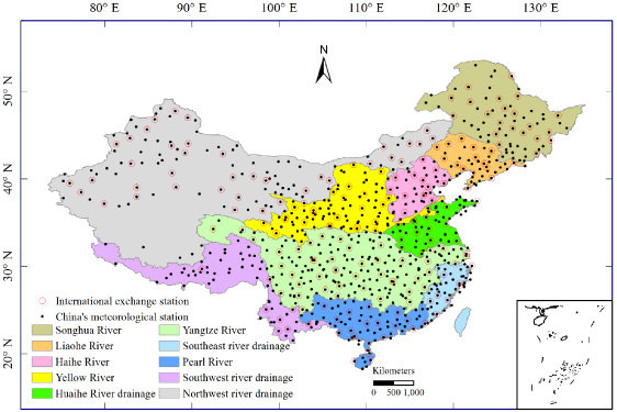
Figure 1. Locations of meteorological stations and major river basins in mainland China.
Download figure:
Standard image High-resolution image3. Results
3.1. Comparison on a temporal scale
Figure 2 shows the time series of annual mean PR and annual mean SAT among all datasets. For PR, it is obvious that these datasets represent different characteristics before and after the 1950s. Before the 1950s, the oscillatory characteristics of annual mean precipitation from three datasets are similar, but the change trends are different. The change rates of annual mean precipitation from CRU, UDEL, and GPCC are 3.107, − 10.998 and − 13.773 mm per decade, respectively. The consistency among datasets is enhanced after the 1950s, represented by totally identical annual variation characteristics and similar trends. The phenomena may relate to the poor instrumental observations in the first half of the 20th century or the more available station observations after the 1950s (Li et al 2012, Wen et al 2006). The observation pre-1950s include strong inhomogeneities due to the lack of a uniform measurement standard (Ge et al 2013), and these three datasets adopt observation data discriminatively (table 1). The rates in this period vary from − 0.019 to 7.556 mm per decade. The change rate of UDEL is highest, and most of the rates identified by different datasets are approximately 2.0 mm per decade, except PREC/L with − 0.019 mm per decade. In the same time period 1962–2006, EA and APHRO present the highest and lowest annual mean PR. For SAT, all datasets indicate an undulating rise overall (figure 2(b)). However, different characteristics of SAT occur in different periods. The upward rates of SAT before the 1950s are small, and the change rate values of CRU and UDEL are 0.116, 0.146 °C per decade, respectively. During 1951–1970, IAP shows a significant negative trend (− 0.897 °C per decade). A slight decrease is evident in UDEL, and CRU, and the values are − 0.153, − 0.107 °C per decade, respectively. Temperatures rise after the 1970s, with SAT rates of change of approximately 0.3 °C per decade. Thus, the SAT dynamic is more intensified after the 1950s than before, which could be primarily attributed to the anthropogenic forcing (Ding et al 2007). For the 45-year mean SAT in 1962–2006, CRU and UDEL is remarkably higher than that in CN05 and IAP. Overall, all PR and SAT datasets show relatively similar varying trends during the most recent 50 years. The spread of the PR dataset is larger than that of the SAT dataset. All SAT datasets indicate that there are two phases of rising temperatures during the past century. The first is from the 1910s to the 1940s and the second is from the 1970s to the present, and at a faster rate.
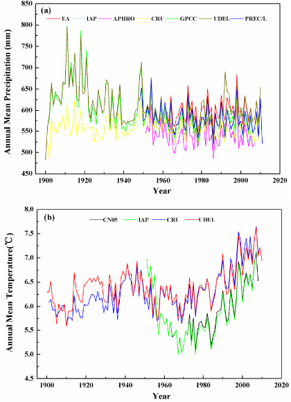
Figure 2. Temporal comparison of annual mean PR (a) and annual SAT (b) among different datasets.
Download figure:
Standard image High-resolution imageThe Taylor diagram provides a method for plotting a 2D graph with three statistics (correlation coefficient (R), standard deviation (SD), and root mean square difference (RMSD)). With the help of the diagram, it is easy to indicate how closely a pattern matches the references (Taylor 2001). In the Taylor diagram, it is generally accepted that a smaller distance between the reference object and the compared object means a closer agreement. Figure 3 displays the agreement of 45-year annual mean climatology (PR and SAT) between the reference and other datasets. For PR, the high R, similar SD and RMSD value again proves the similarity of annual precipitation dynamics. All the correlation coefficients are concentrated from 0.75 to 0.99. IAP and GPCC show the best agreement with EA. Comparably, the UDEL and APHRO datasets are relatively less consistent with EA; their correlation coefficients are less than 0.9. And higher RMSD and SD for UDEL and APHRO represent larger different and more intense inter-annual variability than the other datasets, respectively. For SAT, the Taylor diagram shows that the agreement between CN05 and CRU is still better than that between CN05 and UDEL. Overall, the agreements of CRU and UDEL on SAT are better than that on PR.
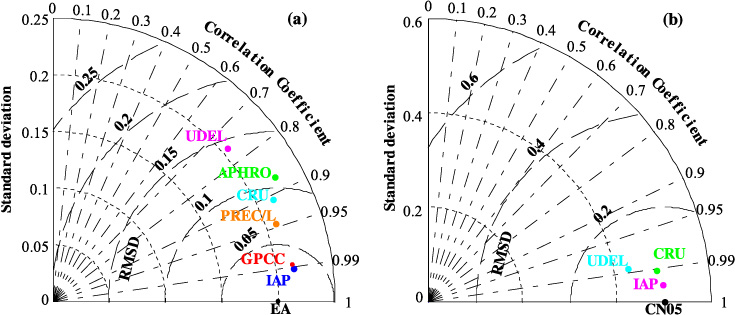
Figure 3. The comparison among datasets based on Taylor diagrams ((a) PR; (b) SAT).
Download figure:
Standard image High-resolution image3.2. Comparison on a spatial scale
The large-scale distribution patterns of the 45-year average precipitation are very similar among the datasets. All datasets display the characteristic that PR gradually decreases from the southeast to the northwest regions (figure 4, left). However, the maximum value (MV) of the 45-year average PR and the location where it appears are dissimilar among the datasets. The MV is ∼2500 mm in APHRO, CRU and IAP, ∼3930 mm in PREC/L, and ∼5000 mm in GPCC, EA, and UDEL. Collectively, heavy rainfall events across the southern Southwest river drainage system have been shown in EA, PREC/L, UDEL and GPCC, but not in CRU, IAP and APHRO.

Figure 4. Spatial distribution of the 45-year (1962–2006) average precipitation (mm) (left) and the difference (right) between EA and the other six gridded precipitation datasets in mainland China.
Download figure:
Standard image High-resolution imageFigure 4 (right) indicates the difference in the 45-year average PR between EA and other datasets. It is obvious that all the datasets show lower PR in most parts of China when compared with EA, especially in the eastern Tibetan Plateau, the northern Northwest river drainage system and southeastern China. The lower PR for CRU, GPCC, PREC/L, and UDEL is more significant in the Tibetan Plateau. The seasonal differences between EA and other datasets are shown in figure 5. Seasonal differences display almost similar phenomena to the 45-year average PR. EA also exhibits a slightly higher amount of PR in all seasons over the eastern Tibetan Plateau, the northern Northwest river drainage system and southeastern China. In CRU, GPCC, PREC/L, and UDEL, the higher amount of PR spreads across the Southwest river drainage system and the southern Northwest river drainage system. The difference in summer is higher than in the other seasons. The climate of China is strongly influenced by the east Asian monsoon (Zhou et al 2010). Moisture transport associated with the Asian summer monsoon is crucial for the China rainfall distribution (Liu et al 2008), and summer is the rainy season in China. Summer corresponds to high precipitation amounts, resulting in the large differences. Thus, the contribution of annual mean PR difference primarily comes from summer.
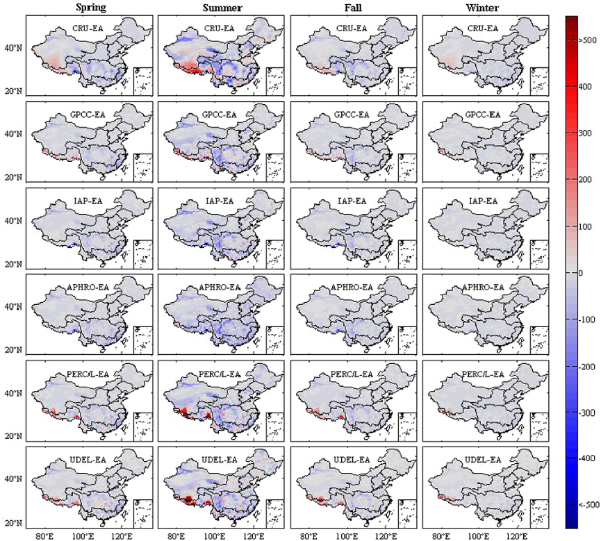
Figure 5. Spatial distribution of the 45-year (1962–2006) average temperature (°C) (left) and the difference (right) between CN05 and the other three gridded temperature datasets in mainland China.
Download figure:
Standard image High-resolution imageFor SAT, all datasets exhibit similar distribution patterns for the 45-year average temperature in mainland China (figure 6, left). In the eastern region, the datasets have relatively little discrepancy with regard to the 45-year average SAT and seasonal distribution (figure 6, right, figure 7). Compared to CN05, CRU shows a higher SAT in the central and southern Northwest river drainage basin, UDEL exhibits a higher SAT over the Southwest river drainage system, and IAP has a lower SAT in the Tibetan Plateau, especially for IAP in winter. Overall, a significant difference occurs in western China, where the largest topographic gradient exists. The seasonal contribution to the 45-year average SAT difference is distinct (figure 7). The contribution coming from winter is slightly larger than the other seasons.
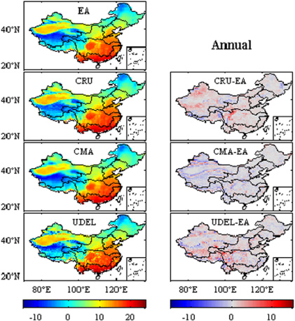
Figure 6. Spatial distribution of the seasonal mean precipitation difference (mm) between EA and the other six gridded precipitation datasets in mainland China during 1962–2006.
Download figure:
Standard image High-resolution image
Figure 7. Spatial distribution of the seasonal mean temperature difference (°C) between CN05 and the other three gridded temperature datasets in mainland China during 1962–2006.
Download figure:
Standard image High-resolution imageFigures 8 and 9 present the spatial correlation in annual and seasonal anomalies of PR and SAT, respectively. For annual and seasonal PR, most datasets show high correlation with EA in the Southeast river basin, with a high correlation coefficient (R > 0.9 for each grid). Relatively higher correlations are observed in GPCC and IAP. However, interesting results can also be observed in IAP and EA, which utilize the same station observation in the Northwest and Southwest river basins, but where relatively low correlation (R < 0.9) appeared. The inconsistency could be mainly due to the design of the interpolation strategy and the interpolation algorithm applied (table 1). In the southern Northwest river basin, the PR correlation phenomena with EA are different among different datasets. It is evident that the PR correlation between CRU and EA is weaker than the other datasets, with a value below 0.9 in most basins, especially in the Northwest river basins. Lower correlations are found in winter than in the other seasons. The inconsistency between CRU and EA covers the Songhua River basin, the Haihe River basin, the Liaohe River basin, the Yellow River basin, and the Southwest and Northwest river drainage systems in winter. Some grids with a zero anomaly value appear in the Northwest river drainage system in CRU, which directly results in the blanks in figure 8. The locations of zero anomaly values vary from season to season, and the area in winter is larger than in the other seasons. For SAT, CRU and UDEL in the Southwest river drainage system, the southern Northwest river drainage system and the upper Pearl River basin show a more remarkable discrepancy than in the other basins. In the southern Northwest river drainage system, low correlation coefficient values occur in IAP.
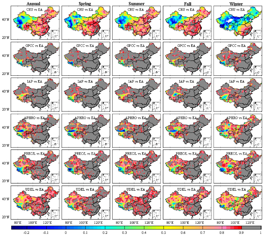
Figure 8. Spatial correlation between EA and other PR datasets on the annual and seasonal anomalies in mainland China during 1962–2006. (The baseline is 1970–1999, and the blank in CRU means no data.)
Download figure:
Standard image High-resolution image
Figure 9. Spatial correlation between CN05 and other SAT datasets on the annual and seasonal anomalies in mainland China during 1962–2006. (The baseline is 1970–1999.)
Download figure:
Standard image High-resolution imageOverall, the consistency in SAT between the reference and other datasets is better than that in PR, displaying higher correlation coefficients in most basins (figure 9). It is also found that the agreements of CRU and UDEL in SAT are better than in PR when compared with the reference. IAP shows relatively weak correlation in PR and SAT in the southern Northwest river drainage system. For seasonal correlation, better performance occurs in spring in PR and SAT.
Moreover, the biases among datasets for monthly PR and SAT anomalies at different quantiles are analyzed. Compared with EA, other datasets tend to have a distribution with lower values for the 90th percentile and higher values for the 10th percentile over larger regions for January precipitation (figure 10). That is, in most regions, EA exhibit higher precipitation for the high percentile but lower precipitation for the lower percentile. The differences in July are relatively higher and broader in magnitude and range, respectively (figure 11). The distribution of biases concentrates on the − 10–10 mm and − 50–50 mm in January and July respectively. The distribution of differences in January and July among six datasets is subtle, except for the CRU datasets. CRU shows higher absolute differences both in the low and high percentiles, and produces a cumulative probability distribution function (CDF) that has a much larger range than the other datasets. For SAT, compared with CN05, the cumulative percentage of hot biases are almost equal to the percentage of cold biases for the 90th and 10th percentiles (figure 12). However, the ranges of CDFs for the 10th percentile are larger than the 90th percentile, with a high absolute difference (>1 °C) existing in the lower percentile. The differences in July are not distinct, with a narrowed range of CDFs and a lower magnitude of bias (figure 13). A higher density of absolute difference for all datasets around 0 °C is obtained compared with January.
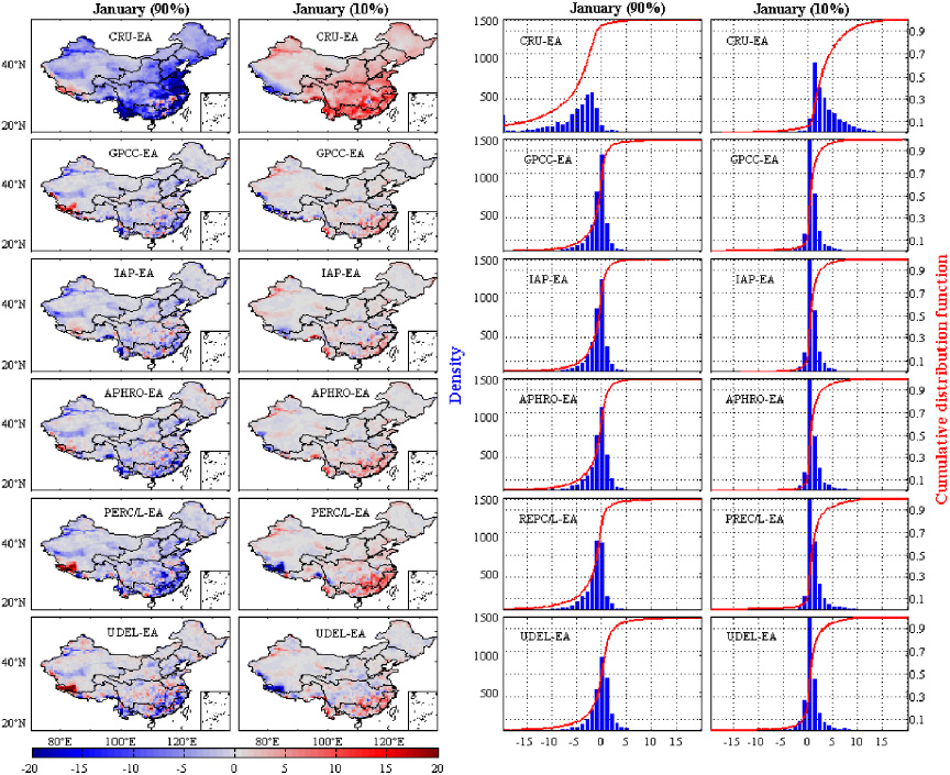
Figure 10. Mean biases for the 90th percentile and 10th percentile (monthly precipitation anomalies) for January (left), and histograms and empirical cumulative distribution function (CDF) of dataset biases (right).
Download figure:
Standard image High-resolution image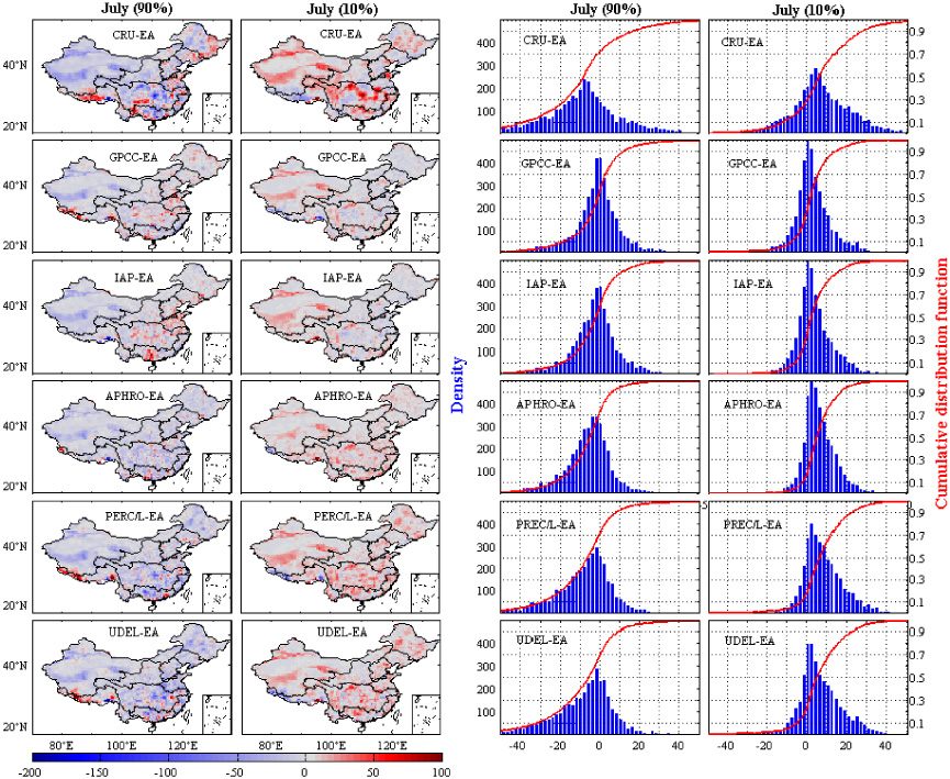
Figure 11. Mean biases for the 90th percentile and 10th percentile (monthly precipitation anomalies) for July (left), and histograms and empirical cumulative distribution function (CDF) of dataset biases (right).
Download figure:
Standard image High-resolution image
Figure 12. Mean biases for the 90th percentile and 10th percentile (monthly temperature anomalies) for January (left), and histograms and empirical cumulative distribution function (CDF) of dataset biases (right).
Download figure:
Standard image High-resolution image
Figure 13. Mean biases for the 90th percentile and 10th percentile (monthly temperature anomalies) for July (left), and histograms and empirical cumulative distribution function (CDF) of dataset biases (right).
Download figure:
Standard image High-resolution image
4. Discussion
In general, several potential factors influence the spatial–temporal agreement among different datasets. The first factor is the source of the raw data used to construct the gridded data. Table 1 shows the involved data sources are different for different datasets. Gauge observations from over 700 Chinese meteorological stations archived by the China Meteorological Administration (CMA) are utilized to construct IAP, CN05 and APHRO. In addition to these stations, EA also uses daily gauge data at over 700 hydrological stations from the Chinese Yellow River Conservation Commission (YRCC) and the Global Telecommunication System (GTS) network. The total number of stations involved is over 2000 for EA. Thus, when compared with those datasets (CRU, UDEL, PREC/L) developed using only ∼200 international exchange stations (figure 1), EA, IAP and APHRO provide more detail on a finer scale (figures 4, 6, left). In addition to the meteorological stations in China, those datasets with larger coverage (such as GPCC, CRU, EA, etc) also contain climate information from neighboring countries when interpolating gridded climate data located near the China boundary. Consequently, the maximum values of the 45-year average PR for EA and APHRO are located in southwest China, while the maximum value occurs in southeast China for IAP. Much more raw data and the national boundary effects may partly contribute to the more significant negative trend during 1951–1970 than CRU and UDEL. In countries neighboring China, the end of the day varies from + 06 UTC (Universal Time Coordinated) to + 09 UTC. Therefore, the analysis derived from their gauge reports may exhibit discontinuities across national boundaries (Xie et al 2007), which partly explains the relatively lower correlation coefficients at the boundaries with India and Russia. Furthermore, the distribution of meteorological stations is sparse in western and northwestern China, which results in larger differences in these regions, especially in the Tibetan Plateau. A large difference appears in the dataset comparison before the 1950s and the consistency among datasets is enhanced after the 1950s (for both PR and SAT) (figure 2). This is largely due to the poor instrumental observations and the uncertainty of the quality of observations in the first half of the 20th century and the more available station observations after the 1950s (Li et al 2012, Wen et al 2006).
The second factor is the quality control (QC) scheme. Because the raw data used to construct the datasets comes from different sources, and meteorological records often contain inhomogeneities, QC is a necessary technique to eliminate unqualified observation data and retain acceptable data to implement the interpolation process. Several non-climatic factors can cause inhomogeneities: changes in measurement practices, station relocation, changes in the station's surroundings over time, etc (Ducre-Robitaille et al 2003). Different QC schemes are applied to confirm consistency in the time series and the quality of datasets. In CRU, all data are subjected to a two-stage quality control process prior to and during interpolation. In APHRO, the QC processes are used to reject data outside the national boundary. In PREC/L, monthly precipitation data with erroneous, questionable or redundant values are removed. In GPCC, the collected data are imported into a relational database and any time new data are imported to the database, an elaborate procedure compares the accompanying metadata of the stations to the metadata already available for that station in the database (Rudolf et al 2009). These different QC processes inevitably influence the agreement among the different datasets.
The third factor is orographic correction (OC). The topographic effect is another important factor relevant to the quality of datasets. Simple interpolation of station observations yields an underestimation of total precipitation, especially over mountainous areas; bias of interpolated temperature is usually in proportion to the increase in local elevation and topographical complexity (Zhao et al 2008). There are many uncertainties in the interpolated observations in western and northwestern China due to the lack of observational coverage and the complex terrain. For PR, parameter-elevation regressions on independent slopes model (PRISM) monthly precipitation climatology is applied to correct the orographic effects in the construction of EA. Compared with other datasets without bias correction for orographic effects, EA shows a relatively higher amount of precipitation over the mountainous areas of southeastern China and along the center of the northwest river drainage system. For SAT, the interpolated surface temperature was calibrated using topographic correction in a similar way to that used in the North American Land Data Assimilation System (Zhao et al 2008) in the construction of the IAP datasets. IAP shows larger cold zones in western China, where higher elevation and complex terrain occur.
The fourth factor is the interpolation technique. In general, the interpolation technique means the interpolation objective and algorithm, which also impact the interpolation performance of gridded datasets (Chen et al 2002). Interpolation objectives primarily include the absolute meteorological value, the anomaly based on average climatology, and the ratio of the observation to the climatology. In this study, the anomalies are interpolated in PREC/L, CRU, and GPCC (version 5), while IAP directly interpolates the observed absolute meteorological value, and EA and APHRO interpolate the ratio. The influence of the interpolation algorithm was confirmed by comparing different interpolation algorithms in a pre-existing study (Chen et al 2002). For PR in western China, EA, IAP and APHRO utilize the same raw data, but large differences occur. For SAT, although the same raw data are used in constructing CN05 and IAP, differences still occur (figure 9). The differences are mainly due to the design of the interpolation strategy and the interpolation algorithm applied (table 1). For IAP, the observed temperatures from gauging stations are interpolated by the common Kriging technique, which uses models of spatial correlation and can be formulated in terms of covariance or semivariogram functions (Childs 2004). For CN05, a gridded climatology is calculated first by using thin-plate smoothing splines, and then a gridded anomaly generated by angular distance weighting (ADW) interpolation is added to obtain the final data (Xu et al 2009). CRU adopts the same interpolation algorithm as CN05; however some differences between CRU and CN05 occur. This is mainly due to the different sizes of the raw data (∼200 observation stations for CRU and 751 for CN05), the different baseline periods used in establishing the anomaly climatology (1961–1990 for CRU and 1971–2000 for CN05), and the selection of different interpolation domains (Xu et al 2009).
It is worth noting that the difference between CRU and the reference object dataset is relatively larger than that between other datasets and the reference object dataset, which is possibly related to the CRU construction process. In CRU, to ensure that the interpolated surface did not extrapolate station information to unwarranted distances, 'dummy' stations with zero anomalies were inserted in regions where there were no stations or synthetic estimates within the correlation decay distance (450 km and 1200 km for PR and SAT, respectively, in CRU); thus, the gridded anomalies were 'relaxed' to zero (Mitchell and Jones 2005). Therefore, the mean in the baseline period (1961–1990) replaces the interpolated gridded value within the distance if there is no other station present. So, in some regions where stations are sparse, such as the Northwest river drainage system, zero anomalies occur, especially for PR. This could result in the occurrences of no data when calculating correlation coefficients (R) in annual and seasonal anomalies between CRU and EA (figure 8). Furthermore, if more than 25% of the values from 1961–1990 were missing for any single calendar month in CRU, then the normal value was not calculated so as to avoid an inaccurate estimation (Mitchell and Jones 2005). As a result, the number of missing observations varies in different months, which may lead to changes in the location of the no-data grid in different seasons.
Recently, many studies have shown that urbanization affects the representativeness of temperature station records (Jones et al 1999). The urbanization effect does not appear to be as marked in the northern hemisphere, most likely because of the more extensive network of nonurban stations and the fact that urban warming was already underway to some extent in the first half of the century (Jones et al 1989, 1990, New et al 2000). However, China is a developing country and has experienced rapid urbanization and dramatic economic growth since its reform process started in late 1978 (Zhou et al 2004). Some studies considered that urbanization in China has had a significant impact on surface temperature trends during the past half century (Li et al 2004, Ren et al 2008, 2010). As the basis of gridded datasets, the observations from stations record the impact to some extent (Ren et al 2005). Thus, the choices of station networks and homogenization to remove urbanization effects are steps to take into consideration in constructing the gridded climate dataset over China.
5. Conclusion
In this study, the similarities and differences of different gridded datasets in presenting the variability of PR and SAT in mainland China are compared. The results show that all datasets can succeed in exhibiting temporal changes in terms of PR and SAT and the characteristics of spatial patterns as a whole. However, there are differences in different datasets. On a temporal scale, EA shows a higher amount of PR, while APHRO shows lower PR when compared to the others. UDEL shows higher SAT than IAP and CN05. On a spatial scale, the most significant differences occur in western China in PR and SAT, especially in the southwestern Southwest river drainage system and the southern Northwest river drainage system. For PR, all the datasets show a lower amount of PR in most parts of China when compared with EA. IAP and GPCC are the most similar to EA, while the difference between EA and CRU is the largest. Compared with CN05, CRU shows higher SAT in the central and southern Northwest drainage basin, UDEL exhibits higher SAT over the Southwest river drainage system, and IAP shows lower SAT in the Tibetan Plateau. Overall, the contributions of annual mean PR and SAT differences mainly come from summer and winter, respectively. The differences in raw data sources, quality control (QC) schemes, orographic correction and interpolation techniques explain the dissimilarities among different datasets. All of these results bring about a new challenge in the field of climate change. So-called 'observed climate datasets' play important roles in driving hydrologic models, evaluating global circulation models (GCMs) and regional climate models (RCM). Because observations coming from different datasets do have differences, which one we can believe among the various so-called 'observed climate datasets'? Indeed, we have no ability to know the 'truth value'; what we need to do is reduce the disagreement among the 'observed datasets' and depress their uncertainty. We think we can firstly quantify the uncertainty of each data set, then understand what caused it. Secondly, we should have good knowledge of the random and systematic error structures of the raw data, which is crucial to ensure successful execution of the generation process. Thirdly, more data sources (such as gauge-based analysis, satellite estimates, proxy data, etc) can be applied to improve the reliability of datasets, especially in regions where observation stations are sparse. Furthermore, correcting the spurious effect of China's remarkable topographical gradients on the datasets improves the accuracy of interpolation. All of these will improve our ability to validate the reliability of climate data in the future, and as a consequence reduce the differences between the different datasets.
Acknowledgments
Funding for this research was provided by the National Key Basic Special Foundation Project of China (2010CB951604) (2010CB428402), the National Natural Science Foundation of China (no. 41001153) and State Key Laboratory of Earth Surface Processes and Resource Ecology. We are grateful to the products' developers for providing the gridded climate data sets.