

Abstract
Although it is generally believed that the increase in the mean global surface temperature since industrialization is caused by the increase in green house gases in the atmosphere, some people cite solar activity, either directly or through its effect on cosmic rays, as an underestimated contributor to such global warming. In this letter a simplified version of the standard picture of the role of greenhouse gases in causing the global warming since industrialization is described. The conditions necessary for this picture to be wholly or partially wrong are then introduced. Evidence is presented from which the contributions of either cosmic rays or solar activity to this warming is deduced. The contribution is shown to be less than 10% of the warming seen in the twentieth century.
Export citation and abstract BibTeX RIS

Content from this work may be used under the terms of the Creative Commons Attribution 3.0 licence. Any further distribution of this work must maintain attribution to the author(s) and the title of the work, journal citation and DOI.
1. Global warming from increased atmospheric greenhouse gas concentrations [1]
1.1. The standard picture
The equilibrium heat balance of the Earth is maintained by the re-radiation of thermal energy, mainly in the infrared (IR) range, at the same rate as the energy falling on it from the Sun which is mainly in the visible part of the spectrum.
The principle components of the atmosphere are nitrogen and oxygen which are diatomic gases whose symmetric molecules have zero electric dipole moment (from the principle of time reversal invariance). In consequence vibrational modes are not excited and these gases do not absorb in the IR. In contrast, triatomic molecules with asymmetric degrees of freedom, such as carbon dioxide (CO2) and water vapour (H2O) allow vibrational modes to be excited by IR radiation. In consequence, these act as strong absorbers of the Earth's IR radiation so that the atmosphere appears almost as a black body to such radiation. To maintain equilibrium the Earth radiates as a black body at an equilibrium temperature of 255 K. With zero CO2 in the atmosphere, the Earth would be a colder place and less hospitable to life. A small amount of CO2 allows the atmosphere to act as a blanket warming the Earth to its more hospitable temperature.
The presence of CO2 and water vapour makes the atmosphere a strong absorber of IR radiation. Direct sunlight (mainly visible wavelengths) penetrates the atmosphere with little absorption and warms the surface of the Earth, the re-radiation from which warms the atmosphere because of this absorption. The atmosphere itself then re-radiates both upwards and downwards from layer to layer. However, at high altitude the pressure becomes small enough that the thickness of atmosphere to outer space is less than one absorption mean free path for IR radiation. At this altitude the IR is radiated to outer space and the temperature (∼255 K) is that at which the energy radiated by the Earth equals the energy falling on it from the sun to maintain equilibrium. At such an altitude water vapour plays little part since it has frozen out at lower altitudes.
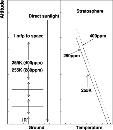
The CO2 is well mixed in the atmosphere. Before industrialization the CO2 concentration was 280 ppm by volume and has increased to 400 ppm today. The effects of this are illustrated by the simple heuristic model shown in figure 1. Adding more CO2 increases the altitude at which there is of order one mean free path to outer space i.e. increases the altitude at which re-radiation to space takes place. The thermodynamics of the atmosphere imposes a linear variation of temperature with altitude with fixed slope, dT/dh, known as the lapse rate [1]. This is fixed by the gas laws. Hence simple geometry shows that increasing the altitude of radiation to space together with the fixed lapse rate will cause the surface temperature of the Earth to increase (see figure 1 right hand box).

Figure 1. Illustration of the simplified model of the production of global warming by increased CO2 concentration from 280 to 400 ppm. The left hand box shows the unabsorbed radiation from sunlight falling on the ground which then re-radiates in the infrared (IR). Strong absorption of IR due to greenhouse gases takes place and the warm atmosphere radiates from layer to layer (represented by horizontal bars). When the atmosphere becomes so thin that there is less than 1 IR mean free path (mfp) to outer space, absorption ceases (layer labelled 255 K, 280 ppm). At this level the temperature is 255 K and there is equilibrium between the energy radiated from the Earth and that received from the Sun. Adding CO2 to the atmosphere decreases the IR mfp so that radiation to space takes place at a higher altitude, the dashed bar labelled 255 K 400 ppm. The right hand box shows temperature (x axis) versus altitude. The temperature in the stratosphere is nearly constant but varies linearly at lower altitude with a fixed slope (the lapse rate) [1]. Increasing the altitude at which the radiation to space occurs moves the temperature contour to the right hand dashed line thus increasing that at the Earth's surface.
Download figure:
Standard image High-resolution image1.2. Quantification of this model and the role of feedback mechanisms
The vibrational modes of molecules such as water and CO2 give rise to absorption of IR radiation in bands of closely spaced lines. Temperature and pressure broadening of the lines cause them to merge together at atmospheric temperatures and pressure. According to the random band model for such absorption [2] the fraction of the radiation transmitted (transmittance T) through a thickness u (at atmospheric pressure) of gas is

where S atm−1 cm−1 is a constant known as the line strength, u is the gas thickness at 1 atmospheric pressure (in atm cm), δ is the line spacing in cm−1 and α is the line width in cm−1. In the strong absorption case, Su/πα ≫ 1, so that  .
.
We now compare the absorptions in the two cases of an atmosphere with CO2 concentration of a1 = 280 ppm and one with a concentration of a2 = 400 ppm. In each case, radiation to outer space from the atmosphere will commence at an altitude at which the air reaches a density such that the mean free path τ is of order unity. Let the air thicknesses at 1 atmosphere pressure for unit absorption mean free path (τ = 1) for these be u1 and u2 in each case, so that the absorber thicknesses are a1u1 and a2u2. It follows that

and hence

The mass of a column of air of thickness u at 1 atmosphere pressure above an area dS is ρAu dS where ρA is the density of the air at 1 atmosphere pressure. The real atmosphere has a variable density so the mass above altitude z is  . They have the same mass so for unit area dS = 1 m2 (dS cancels)

Assume that the air is an ideal gas with PV = mRT so that density ρ = P/RT and  where H is the scale height of the atmosphere. We take the scale height H to be approximately independent of altitude above the tropopause and assume that the atmosphere is at a constant absolute temperature. Such approximations are good to of order 20% accuracy. Hence equation (4) becomes

i.e.

Substituting this into equation (3) and assuming that the line width α varies linearly with pressure i.e.  where k is a constant, we see that

where z1(z2) is the altitude for radiation to outer space at CO2 concentration a1(a2). Taking logs gives

i.e.

The conclusions of this simple reductionist model is that the increase of the CO2 from a1 = 280 ppm to a2 = 400 ppm gives Δz = 1.1 km for a scale height (above the tropopause) of 6.35 km. For a lapse rate of 6 K km−1 this gives a temperature rise of 6.6°.
Such a temperature rise is much larger than the observed increase of 0.8° seen since industrialization. To explain this difference feedback mechanisms and all the other complications of the climate need to be invoked. Some of these complications serve to reduce the temperature increase and some to decrease it. Presumably the mechanisms which decrease the rise have a greater effect than those which increase it so that the actual rise in temperature is smaller than that predicted by the simple model.
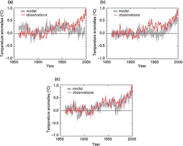
Note that this is a grossly simplified, reductionist model of the global warming which has occurred since industrialization. In practise, the Earth's climate is much more complicated with many different effects occurring simultaneously. Such effects are modelled in general circulation models (GCM) of the climate which include all known processes (including the one described above). Figure 2 [4] shows the results of these models compared to the measured mean global surface temperature. There is a good agreement between the measurements and the model calculations. However, if the effects of the increase in green house gases are ignored, as in the upper left hand panel of figure 2, then the models do not agree with the data.

Figure 2. The red curves show the measured global mean temperature anomaly as a function of date while the grey curves show the results of general circulation models of the climate. The grey curve in the upper left hand panel (a) shows the model calculations with only natural forcings. The upper right hand panel (b) grey curve shows the effects of the anthropogenic forcings only and the lower panel (c) the combination of natural and anthropogenic forcings. The spread of the grey curves shows the results from several models overlaid [4].
Download figure:
Standard image High-resolution image1.3. How could this picture of man-made global warming be wrong?
For the picture to be wrong, the effects of the increased CO2 in the models of the climate must be wrong and the models, if they were correct, ought to produce results similar to the grey curves in the upper left hand panel (a) of figure 2. In that case there would have to be a process which is not included in the models. Since the models should include all known phenomena the process is presumably unknown to climate science at present.
Furthermore, the process or processes must reproduce the warming seen since industrialization rather than cooling. Such a chain of conditions reduces the probability that this is the state of things even though any one of the three conditions is not so improbable.
The Intergovernmental Panel on Climate Change (IPCC) [3] say that 'it is extremely likely that human influence has been the dominant cause of the observed warming since the mid 20th century' due to the observed increase in anthropogenic green house gas concentrations. Here 'extremely likely' is defined as more than 95% probable. Hence it is less than 5% probable that most of the warming is due to natural causes.
Let us suppose that the standard picture is wrong. We can then ask if solar activity or cosmic rays is the new effect which would cause the majority of the observed warming.
2. Searches for a solar/cosmic ray effect on the climate
2.1. Prehistoric searches
Palaeontological effects hinting at a connection between cosmic rays and the Earth's climate in the distant past have been reported. One clear correlation between the cosmic ray rate as measured by the 14C data from ancient trees and monsoon rainfall from 18O data is reported by Neff et al [5] from 9500 to 5500 years ago. This correlation is very sensitive to the local wind strength and direction and is thought to indicate a connection between the North Atlantic oscillation and solar activity. This affected the local monsoon rainfall at the epoch but it is unclear if it affects the climate as whole.
Another correlation was noted by Shaviv and Veizer [6]. They took the computations of a model by Shaviv [7] of the changes in the cosmic ray flux as the Solar System moves from one spiral arm of the Galaxy into the inter-arm region. They compared these fluxes with prehistoric temperature variations deduced by Veizer from 18O data and noted a distinct correlation. This work was criticized by Overholt et al [8] on the grounds that the Sun crossed the Galactic Spiral arms at different and irregular times rather than at the times proposed by Shaviv which had a regular period. Furthermore, Shaviv's model predicts a ratio of cosmic ray intensities in the spiral arm to inter-arm regions of 3:1. This seems excessive given that the scale height of the arms is roughly similar to the inter-arm separation. Hence, using the conventional picture of the Galaxy this ratio would expected to be much smaller and of order 20% [9]. Here, the scale height is the standard deviation of the distribution of cosmic rays about the centre of the spiral arms.
In conclusion, the palaeontological evidence for a correlation between cosmic rays and the global temperature is weak and confused. In addition, in those ancient times many other things were different than today such as the orientation of the Earth's orbit, Earth's atmosphere etc. Hence it is difficult to use such evidence to verify a modern connection between cosmic rays and the climate.
2.2. A modern correlation
A more modern correlation between the solar modulation of the cosmic ray rate, as measured from neutron monitors, and the low level cloud cover (measured from the ISCCP IR data) [10] during the period 1983–1995 (solar cycle 22) was noted by Svensmark et al [11, 12]. Here the neutron monitor data were used as a proxy for the ionization rate in the atmosphere. Marsh and Svensmark [12] observed a dip in the low level cloud cover between 1983 and 1995 which followed closely the decrease in the neutron monitor data due to the 11 year solar cycle.
They used this correlation to hypothesize that there was a strong connection between the production of clouds and ionization from cosmic rays. They went on to show that, if this were a global phenomenon, it would explain most of the global warming seen in the twentieth century [12, 13]. The cosmic ray rate has been shown to have decreased during the twentieth century [14] so fewer cosmic rays implies less low cloud i.e. more solar radiation penetrating to the surface of the Earth i.e. more warming. However, the correlation was examined by Voiculescu et al [15] who showed that it was not a global phenomenon but that it only existed in certain regions covering a fraction of the globe. Hence the effect can only be used to explain a fraction of the global warming seen in the twentieth century.
3. Searches for evidence to corroborate the hypothesized connection between CR and the climate
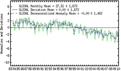
Figure 3 shows the ISCCP IR data used by Marsh and Svensmark [12] for 1983–2010. This includes the following solar cycle 23 which has passed since the observation of the correlation in solar cycle 22 (1983–1995). The data show a gradual decrease in low level cloud cover during the following solar cycle from 1995 to 2010 but there is no dip similar to the one seen from 1983 to 95. Hence the following solar cycle does not corroborate the hypothesis. Furthermore, the hypothesis is not corroborated by another set of cloud data from the ISCCP project [16] where the correlation is not observed.

Figure 3. The ISCCP IR measurements of global mean low level cloud anomalies [10] from the infrared data as a function of time (1988–2010). The blue curve shows the seasonally corrected measurements and the green curve those before seasonal correction.
Download figure:
Standard image High-resolution imageAn examination of the dip in the low level cloud cover in cycle 22 showed that its magnitude was independent of magnetic latitude. If clouds were being influenced by cosmic rays the decrease should have been greater at the magnetic poles than at the magnetic equator since the solar modulation of the ionization from cosmic rays is greater at the poles than at the equator [17]. A statistical analysis of the failure to find a magnetic latitude dependence of the effect showed that less than 23% of the decrease comes from the changing cosmic ray rate at 90% confidence level [18].
Figure 4 shows the variation of the mean global surface temperature compared to the equivalent Climax neutron monitor rate as a function of time since 1890. The equivalent neutron monitor rate has been derived from the 10Be data from ice cores [14]. Here the data have been smoothed by taking an 11 year running mean to illustrate the overall trend and eliminate the effects of the 11 year solar cycle on the neutron data. An examination of the cosmic ray rate shows that the decrease occurred in the first half of the twentieth century when the rate of increase of temperature was small. In the second half of the century the cosmic ray rate change was small while the temperature increased rapidly. Hence the changing cosmic ray rate correlates badly with the rise in temperature. From this it was shown that the contribution of the changing cosmic ray rate is less than 10% of the twentieth century rise in temperature (global warming) [19].
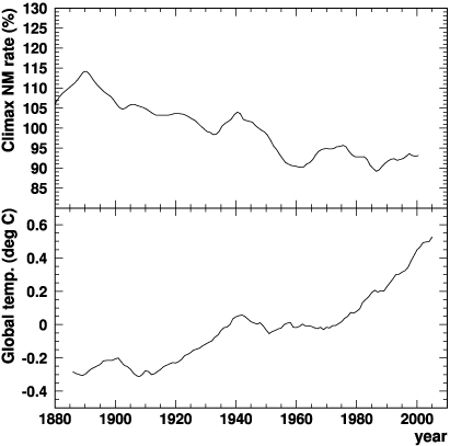
Figure 4. The upper panel shows the equivalent Climax neutron monitor rate deduced from the measurements of 10Be in ice cores [14]. Here the data have been smoothed using an 11 year running mean to remove the 11 year solar cycle. The lower panel shows the mean global surface temperature with the same smoothing applied. It will be noted that since 1960 the CR intensity has only oscillated and not continued on its downward path, whereas the temperature has increased at an accelerated rate.
Download figure:
Standard image High-resolution imageFrom these observations we conclude that the correlation observed by [12] in solar cycle 22 is spurious. However, this is not to say that there is no connection between the varying cosmic ray rate and cloud formation. There could well be an effect there to explain the observations of [20] but if there is a connection between changing cosmic rays and clouds it cannot contribute more than 10% of the global warming seen in the twentieth century.
4. Cloud droplet formation
For pure water the vapour pressure over a curved surface varies according to the Kelvin formula as expa/r where a is a constant related to the surface tension of water and r is the radius of the drop. It is easy for two molecules of water to stick together because of their large electric dipole moments. However, the Kelvin formula means that, to increase in size, the putative droplet would need such a large saturation vapour pressure that growth would not occur. However, droplet growth in the atmosphere can occur via the deliquescent impurities [1]. Here the water molecules stick to the impurities (e.g. a grain of common salt from sea spray) and an aerosol can form. Such aerosols can then grow by coagulation into cloud condensation nuclei.
Ionization of a putative aerosol particle can also act as a centre for growth. It is predicted [21] that ionized sulfate particles can act as centres for the growth of aerosols. Indeed, the CLOUD experiment at CERN has shown that the number of aerosol particles grows with ionization in the presence of sulfuric acid by factors between two and ten as the ionization rate increases from zero to that expected from the cosmic rays [22]. However, the overall rate of aerosol production was observed to be orders of magnitude less than that observed in the real atmosphere unless the temperature is reduced to below a realistic value for the lower atmosphere. However, the rates could be significant in the upper atmosphere where the temperatures are lower and the ionization rate from cosmic rays is higher. We conclude from this that the CLOUD experiment has identified one ionization sensitive process which could influence cloud formation. However, according to the observations by the CLOUD Collaboration [22], this only contributes a small fraction to the overall aerosol production rate in the low level atmosphere.
5. Other searches for the influence of ionization on cloud formation
Mironova et al [23] observed an increase in the stratospheric aerosol production in a limited region of the northern hemisphere a few days after the large ground level event (GLE) of 20 January 2005. However, the observed effect is at too high an altitude to influence cloud formation.
Various other tests were made by our group to search for increases in cloud cover when there were known increases in the atmospheric ionization rate. Searches were made for increased cloud cover around Chernobyl following the nuclear accident in 1986. Searches were made comparing regions of known large radon concentration in India with neighbouring regions where the concentration was low. Searches were made for an increase in the global average cloud cover following the ionization burst from the very large GLE in 1989. There was no indication in any of these searches for an increase in cloud following the ionization release [24].
A further search was also made of the historic records of the nuclear weapons testing programme in the 1950s and 1960s. For example, the BRAVO test was carried out on 1 March 1954 when a very large 15 Mton bomb was exploded in the atmosphere. At a distance of 500 km from the test site the blast wave is negligible. Here, the radiation level was recorded at 20 Rh−1 16 h after the explosion. This corresponds to an ionization rate of ∼107 ion pairs per cm3 per second i.e. many orders of magnitude more than the cosmic ray ionization rate. Detailed observations are available for this region. However, there were no reports of any change in cloud cover or weather pattern for the region following the test. A more general search of all the bomb tests also found no evidence for a correlation between ionization in the atmosphere and cloud production [24].
In conclusion we made numerous searches for a connection between ionizing events and cloud formation but no connection was found [24].
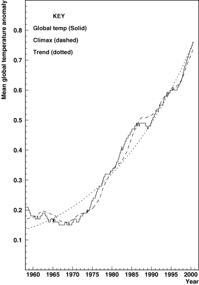
6. A direct search for a link between the mean global surface temperature and solar activity [25]
Figure 5 shows the mean global temperature as a function of time since 1955 (solid curve) together with a trend line to guide the eye (dotted curve). Here the data have been smoothed using an 11 year running average. The mean of the Climax and Huancayo neutron monitors (with the same smoothing) added to the trend line is shown as the dashed curve. Here the neutron data have been arbitrarily normalized and inverted to illustrate the similarity with the temperature data. It can be seen that both the temperature and neutron monitor data show the same tendency to oscillate about the trend line with roughly a 22 year period. The amplitude of the temperature oscillation is ±0.07°. However, the cosmic ray oscillation seems to lag that for the temperature by 1–2 years [25]. Hence, clearly, the changing CR rate cannot cause the temperature change. This lag would indicate that if the correlation is real it is most probably caused by an instantaneous effect such as changes in solar irradiance. It is known that changing solar activity produces changes in the cosmic ray rate which are delayed by 1–2 years.
Let us make the assumption that the oscillation in temperature is produced by the changing solar activity as measured by the cosmic ray rate in figure 5. The long term change in the cosmic ray rate was less than the amplitude of the oscillation in the cosmic ray rate seen in figure 5. Hence the long term change in temperature due to solar activity will be less than the observed amplitude of the oscillation in figure 5. Therefore there is no evidence to suggest the existence of a long term change in the mean global temperature exceeding 0.07 ° C due to changing solar activity, compared to the observed warming of ∼0.5°. This implies that less than 14% of the global warming seen since 1955 is attributable to solar activity.
Figure 5. Global mean temperatures (solid curve), mean of Huancayo and Climax neutron monitor data (dashed curve) arbitrarily normalized and added to the trend line (dotted curve). The mean temperatures and the neutron monitor data have been smoothed using an 11 year running average. Note that the CR rate has been normalized to that of temperature and inverted to illustrate the similarity of the trend. The actual change in CR rate over this period is only about 4% (see figure 4).
Download figure:
Standard image High-resolution image
7. Conclusions
Numerous searches have been made to try establish whether or not cosmic rays could have affected the climate, either through cloud formation or otherwise. We have one possible hint of a correlation between solar activity and the mean global surface temperature. This is comprised of an oscillation in the temperature of amplitude ±0.07° in amplitude with a 22 year period. The cosmic ray data show a similar oscillation but delayed by 1–2 years. The long term change in the cosmic ray rate is less than the amplitude of the 22 year variation on the cosmic ray rate. Using the changing cosmic ray rate as a proxy for solar activity, this result implies that less than 14% of global warming seen since the 1950s comes from changes in solar activity. Several other tests have been described and their results all indicate that the contribution of changing solar activity either through cosmic rays or otherwise cannot have contributed more than 10% of the global warming seen in the twentieth century.
We conclude that cosmic rays and solar activity which we have examined here, in some depth, therefore cannot be a very significant underestimated contributor to the global warming seen in the twentieth century.
Acknowledgment
We thank the John Taylor foundation for financial support.