
Abstract
This letter documents the development and validation of a climate-driven, southwestern-US-wide water resources planning model that is being used to explore the implications of extended drought and climate warming on the allocation of water among competing uses. These model uses include a separate accounting for irrigated agriculture; municipal indoor use based on local population and per-capita consumption; climate-driven municipal outdoor turf and amenity watering; and thermoelectric cooling. The model simulates the natural and managed flows of rivers throughout the southwest, including the South Platte, the Arkansas, the Colorado, the Green, the Salt, the Sacramento, the San Joaquin, the Owens, and more than 50 others. Calibration was performed on parameters of land cover, snow accumulation and melt, and water capacity and hydraulic conductivity of soil horizons. Goodness of fit statistics and other measures of performance are shown for a select number of locations and are used to summarize the model's ability to represent monthly streamflow, reservoir storages, surface and ground water deliveries, etc, under 1980–2010 levels of sectoral water use.
Export citation and abstract BibTeX RIS

Content from this work may be used under the terms of the Creative Commons Attribution 3.0 licence. Any further distribution of this work must maintain attribution to the author(s) and the title of the work, journal citation and DOI.
1. Introduction
One of the most robustly described impacts of projected climate warming for the southwestern US will be on the water resources of the snowmelt-driven hydrologic systems of the region, which provide water for the 50 million people or nearly 20% of the US population. In the southwestern US, climate change will impact the natural and human systems that rely on the hydrologic character of its snowmelt-driven mountain ranges, from the Rocky Mountains that rise out of Wyoming, Colorado, Utah, New Mexico, and Arizona, to the Sierra Nevada range that spans nearly 700 km across the interior of California. These are the main supply sources that provide water to a state that is the top agricultural producer in the US, taking advantage of its dry, warm summertime Mediterranean climate to irrigate about 36 000 km2 (9000 000 acre) of farmland (Bajwa et al 1992, CDWR 2009). Arizona, Colorado, and Utah are also regions with considerable agricultural production. Hay feed dominates Colorado and Utah irrigated agriculture, with total irrigated area of about 13 700 km2 (3400 000 acre) and 4800 km2 (1200 000 acres) in Colorado and Utah, respectively. Year-round irrigation occurs in the southwestern portion of Arizona, making use of its Colorado, Gila, and Salt river waters and groundwater to irrigate nearly 3600 km2 (900 000 acre), with considerable acreage in cotton, citrus and vegetables, and hay to a lesser extent (Stitzer et al 2009).
The water of the southwestern US is intricately linked, with California arguably the lynchpin of the region's water system. Southern California receives imported water from both the Colorado and the Sacramento-San Joaquin Rivers. Several large California Irrigation Districts such as the Imperial Irrigation District and the Coachella Valley Water District use nearly a quarter of California's available Colorado River water, while water delivered for municipal uses into the Los Angeles Basin and San Diego are about 4% (CDWR 2009). Arizona and Nevada are the other two 'Lower Basin States', which receive the remainder of the share of Colorado River water. The Upper Basin States are apportioned 9250 million m3 or MM3 (7.5 million acre-feet or MAF) among Colorado (52%), New Mexico (11%), Utah (23%), and Wyoming (14%); the portion of Arizona that lies within the Upper Colorado Basin is apportioned 61 MM3 (0.05 MAF) annually. The Lower Basin is also apportioned 9250 MM3 (7.5 MAF) among the states of Arizona (37%), California (59%) and Nevada (4%).
This letter summarizes the development of a southwestern US water systems model built on the Water Evaluation and Planning system platform (Yates et al 2005). This model, hereafter called WEAP-SW represents the water supply and use of more than 60 major river basins throughout Colorado, Wyoming, New Mexico, Utah, Nevada, Arizona, and California (figure 1). The WEAP-SW model is spatially based, capable of calculating changes in the hydrologic cycle, including changes in climate conditions and human interventions such as reservoirs, canals and tunnels, irrigation systems, urban water system, hydropower facilities, etc. This platform allows users to incorporate scenarios of future climate warming and demand use patterns, including changes in irrigated agriculture, urban demand, and thermoelectric cooling demand; and then estimate subsequent impacts and possible adaptation strategies within one platform (Yates et al 2009). In a companion paper (Yates et al 2013), the WEAP-SW model is used to explore the implications of future electricity portfolio scenarios, as represented by the regional energy deployment system (ReEDS) model (Short et al 2011), on the water resources of the southwestern US. Thus, the main purpose of this letter is to lend credibility to the WEAP-SW model, as a valid and useful tool for exploring the relative tradeoff of our energy choices on this tightly integrated water system.
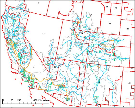
Figure 1. The WEAP-SW domain, with PCA boundaries (red and numbered), trans-basin diversions (orange); rivers (light blue) and watershed boundaries (gray). The inset box shows the location of the area shown in figure 3.
Download figure:
Standard image High-resolution imageThe WEAP-SW model places a particular emphasis on the water used for thermoelectric cooling, which accounts for over 40% of freshwater withdrawals in the United States, principally from plants using once-through cooling (Kenny et al 2009). Withdrawals can be substantially reduced by switching to evaporative or recirculating cooling, but the switch may increase overall consumptive use (Macknick et al 2011). The WEAP-SW model includes an explicit representation of thermoelectric cooling water requirements based on output from the regional energy deployment system (ReEDS) model (see Sattler et al 2012). The ReEDS models estimates electricity capacity and generation at the level of the continental United States' 134 power control authorities (PCAs) for a series of two-year periods between 2008 and 2050 (Short et al 2011).
2. Methodology: WEAP as the analytical framework
The WEAP decision support system (DSS) is an integrated water simulation tool that includes a robust and flexible representation of water demands from all sectors; and allows for the description operating rules for infrastructure elements such as reservoirs, diversions, environmental flows, canals, hydropower, etc (Yates et al 2005). It has watershed rainfall-runoff modeling capabilities that allow for the calculation of hydrologic components including snow accumulation and melt, soil moisture, runoff, interflow, and base flow. Water infrastructure and demand elements can be dynamically nested within the underlying hydrological processes. In effect, this allows the modeler to analyze how specific configurations of infrastructure, operating rules, and priorities will affect water uses as diverse as instream flows, agricultural irrigation, municipal water supply under the umbrella of climate forcing and physical watershed conditions. This makes it ideally suited to studies of dynamic change within watersheds, such as climate warming (Yates et al 2009).
The physical hydrology model in WEAP represents the terrestrial water cycle with a series of simultaneously solved equations. Precipitation is partitioned into snow or rain and runoff, or infiltration depending on temperature, land cover, and soil moisture status. Moisture in the root zone is partitioned into evapotranspiration, interflow, deep percolation, or storage as a function of soil water capacity, hydraulic conductivity, potential evapotranspiration (PET), and vegetation specific PET coefficients. The model simulates soil water evaporation as a function of snow cover, relative soil moisture and an estimate of potential evapotranspiration using the Penman Monteith method (Monteith 1965). Deep percolation enters a deep soil horizon and is partitioned into base flow or storage. This partitioning is a function of the soil moisture storage status and the water holding capacity and conductivity of this deep compartment. For a detailed discussion of the model algorithms see (Yates et al 2005).
Water allocation in WEAP is established through a set of user-defined demand priorities and supply preference that are used to construct an optimization routine that allocates available supplies at each timestep. A linear programming (LP) solver allocates water to maximize satisfaction of demand, subject to supply priorities, demand site preferences, mass balance and other constraints. Demands, reservoir storage, hydropower, and instream flow requirements are assigned a unique integer priority number, ranging from 1 (the highest priority) to 99 (the lowest priority). Those entities with a Priority 1 ranking are members of Equity Group 1, those with a Priority 2 ranking are members of Equity Group 2, and so on. The LP constraint set is written to supply an equal percentage of water to the members of each Equity Group. The Priority Numbers are not weights, but ensure that demands with Priority 1 are allocated water before those with Priority 2, Priority 2 before Priority 3, and so on. In the WEAP-SW model, the priority ranking is given as: Priority 1: instream flow and water compact requirements, and thermoelectric cooling; Priority 2: urban indoor water; Priority 3: urban outdoor water; Priority 4: irrigated agriculture; and Priority 5: hydropower. This priority means that other uses will be curtailed to ensure that flow requirements and thermoelectric cooling water requirements are met under water constrained conditions. The WEAP-SW model makes use of WEAP's internal inked groundwater-surface model to track water fluxes from the surface through the sub-surface demand nodes are then linked to surface water, groundwater, or both, with capacity constraints used to determine the fraction of water supplied from the various sources, primarily based on state and federal data (table 1).
Table 1. Summary of modeled components and associated data sources and assumptions used to develop the WEAP-SW model.
| Model component | Use/assumption | Source |
|---|---|---|
| Rivers/tributaries, watershed boundaries and contributing areas, and hydropower potential | General model development and hydrologic connectivity. Elevations used to determine hydropower potential | The National Hydrography Dataset-Plus (NHD Plus) (www.//horizon-systems.com/NHDPlus/) |
| Land cover categories: forested, non-forested, irrigated agriculture, and urban | 4-land classes are adequate to determine the hydrologic response of the catchment. Used to estimate irrigated acreage | The National Land Cover Dataset (NLCD) 2006 (www.//epa.gov/mrlc/nlcd-2006.html) |
| Gridded climate forcing of monthly total precipitation and monthly average temperature | Climate forcing for each catchment object computed as the average of each catchment's elevation band | The Bias Corrected and Downscaled WCRP CMIP3 Climate and Hydrology Projection Archive (http://gdo-dcp.ucllnl.org) for historic and future climate data |
| Observed monthly average streamflow | Used in model calibration | US Geological Survey for historic water data (streamflow, water quality, water demand, etc http://water.usgs.gov/) |
| Reservoir capacities, head-area-volumes, dam height and tailwater elevations, turbine capacities, hydropower operating criteria | Specification of reservoir capacity and operating procedures. Determination of: reservoir evaporative losses, conservation and flood control storage, and hydropower generation | United States Bureau of Reclamation; Colorado Water Conservation Board; Utah Division of Water Resources; Arizona Department of water Resources; California Department of Water Resources; US Geological Survey |
| Water use: municipal, industrial and irrigated agriculture; water use for thermoelectric generation and cooling. Per-capita water use. Local groundwater availability, attributes, and proportional use | Assumed constant per-capita water demand that represents a withdrawal and a constant fractional use. Local groundwater attributes. WEAP supply priorities applied based on regional descriptions. Local data used to refine agriculture water use; and hydropower production | State and local data resources (Colorado: Colorado Water Conservation Board; Arizona: Arizona Department of Water Resources; Utah: Division of Water Resources; California: California Department of Water Resources, California Energy Commission Water Use and Conservation Bureau, NM) |
2.1. WEAP-SW catchment delineation and climate data
Catchment objects in WEAP were used to represent topographically identified sub-catchments that are characterized by unique climate, land cover–land use (LULC), and soil water properties. The hydrologic model within each sub-catchment was parameterized using publicly available LULC and 100 m digital elevations (DEM; http://seamless.usgs.gov/) data. The LULC data was obtained from the National Land Cover Dataset or NLCD (Homer et al 2004), whose land cover classes were aggregated into five categories. These included forested, non-forested, irrigated agriculture, urban, urban outdoor to allow for the explicit representation of urban outdoor landscape and amenity watering.
The WEAP-SW sub-catchments were created by (1) identifying the major southwestern river basins based on the designation of the USGS Hydrologic Unit Classification system; (2) identifying basin 'pour points' where there is important infrastructure such as dams, diversions, return flow structures, stream flow gages, etc; (3) intersecting 500 m elevation bands within each basin to create WEAP sub-catchments, (4) estimating the total area of each sub-catchment and then classifying within each, the proportional of the LULC as either forested, non-forested, irrigated agriculture, urban, or urban outdoor.
This delineation procedure resulted in 63 river basins, comprising 306 catchment objects in the WEAP-SW model. The sub-catchments averaged 3400 km2 in size, but with considerable variation, as some are more finely discretized to capture important topographic gradients, most notably those in the headwater regions such as the Rocky Mountains and the Sierra Nevada (figure 1). A selection of some of the major river basins included in WEAP-SW is given in table 2. A gridded, continental US climate dataset was used to estimate monthly average temperature and total precipitation for each combination of sub-catchment and elevation band (Maurer et al 2010) for the period 1979–2010 (figure 2). This period was chosen as it represents the point in which the major water infrastructure was in place and Lake Powell had filled.
Table 2. Select watershed names and model information. In some cases, sub-catchments are counted more than once, as they contribute to both the upstream and larger downstream basins.
| Watershed name and code | State | Watershed point or outlet | # of sub-catchments |
|---|---|---|---|
| South Platte R.—SPL | CO | AT DDENVER 06764000 | 3 |
| Arkansas R.—ARK | CO | ABOVE PUEBLO RESERVOIR 07099400 | 4 |
| Rio Grande—RIO | NM | AT OTOWI 08313000 | 6 |
| Upr Colo R.—UCO | CO | UPR COLO NR UTAH 09163500 | 22 |
| Green R.—GRN | UT | AT GREEN 09315000 | 25 |
| Provo—PRO | UT | NR LYNNDYL 10224000 | 4 |
| Colo R.—COP | AZ | LAKE POWELL INFLOW | 83 |
| Salt R.—SLT | AZ | BLW STW MTN RESERVOIR 09502000 | 19 |
| Colo R.—COM | NV | BELOW LAKE MEAD | 98 |
| Colo. R—CIP | AZ | BLW IMPERIAL RES | 122 |
| Pitt R.—PIT | CA | INFLOW TO SHASTA | 5 |
| American R.—AMR | CA | FOLSOM RESERVOIR | 4 |
| San Joaquin R.—SAN | CA | SAN JOAQUIN NR VERNALIS 11303500 | 13 |
| Kern River—KER | CA | KERN RIVER ABV ISABELLA | 7 |
| Sacramento R.—SAC | CA | SACRAMENTO AT DELTA | 54 |
| Total | 306 | ||
| Average area (±SD) | 3400 km2 (4300 km2) |
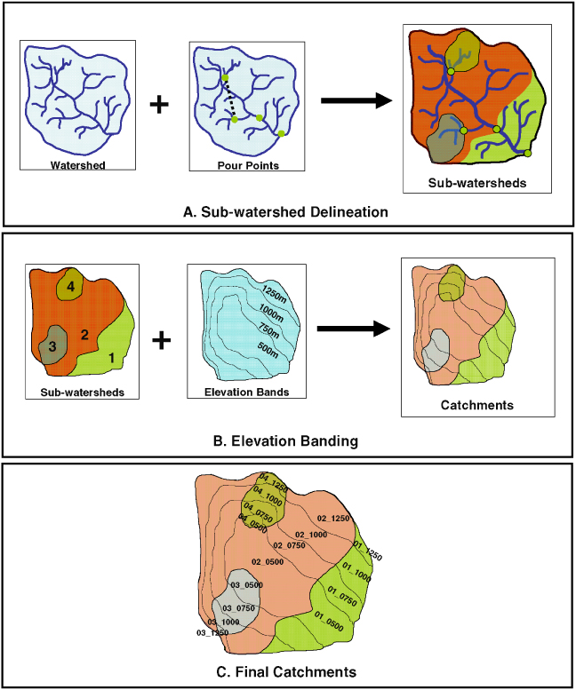
Figure 2. Subwatershed delineation, elevation banding and catchment definition. A unique climate sequence was derived for each sub-catchment_elevation band pair.
Download figure:
Standard image High-resolution image2.2. Water use and infrastructure data
Several data sources were used to configure the model in terms of land use/land cover, regional population, water use, agricultural extent, streamflow, reservoirs, diversions, tunnels, thermoelectric cooling, instream flow requirements, water compacts between states, etc and are summarized in table 1. Monthly water use was simulated for each sector, primarily from state level data with their annual estimates summarized in table 3. The values in this table are important in-as-much as they are represent our best estimate of sectoral demand across the region and are what drive the WEAP-SW model in allocating water among the competing uses. Municipal, commercial, and industrial indoor use (excluding thermoelectric generation) were based on estimates of population and water use per-capita as liters-per-capita-per-day or LPD (gallons-per-capita-per-day or GPD). A value of 265 LPD (70 GPD) was used for residential uses plus an additional 95 LPD (25 GPD) for commercial and industrial indoor use. Some areas were assigned slightly higher per-capita, including the Salt Lake Valley, Phoenix, Las Vegas, and the Los Angeles Basin where an additional 75–115 LPD (20–30 GPD) of indoor use was assumed based on higher estimates from greater industrial or commercial activity or household use estimates (Stitzer et al 2009, DWR 2010, Camp, Dresser, and McKee 2004, CDWR 2009, UDWR 2010, ADWR 2008, 2010, ConSol 2010, CWCB 2009).
Table 3. Column 1 and 2 define the reporting region and summarizes their 2008 population estimates, while column 3 is the irrigated land area for the region. Column 4–6 report the annual delivered water in millions of m3 for each sector; where column 4 is the minimum, maximum, and average water delivered to the agricultural sector; column 5 is the municipal and industrial indoor delivered water (MiI) for 2008 levels of demand; column 6 is the municipal outdoor (MuO) minimum and maximum for the period 1980–2010; and column 7 is the annual water withdrawal for thermoelectric cooling.
| ST | Region (Pop '000000) | Ag area (km2) | Ag applied water (Mn, Mx, Avg) | MiI | MuO (Mx, Mn) | Thermo |
|---|---|---|---|---|---|---|
| Colorado | South Platte (3.5) | 3 200 | 1300, 2100, 1600 | 390 | 235, 460 | 410 |
| Arkansas (1.3) | 1 720 | 1200, 1700, 1400 | 160 | 90, 160 | 103 | |
| West Slope (0.4) | 4 900 | 1500, 2400, 2000 | 63 | 60, 70 | 344 | |
| San Luis (0.1) | 2 100 | 1720, 2200, 1900 | 9 | 7, 10 | 9 | |
| Utah | Salt Lake (2.4) | 2 700 | 500, 980, 740 | 280 | 195, 320 | 280 |
| Colo River* (0.1) | 2 200 | 1250, 1570, 1440 | 25 | 20, 25 | 41 | |
| NM | N./RioGrande (0.9) | 941 | 440, 580, 510 | 170 | 145, 165 | 2500 |
| NV | Las Vegas (1.4) | — | 270 | 236, 280 | 59 | |
| Arizona | Grt Phoenix (4.0) | 2 000 | 1500, 2300, 1800 | 425 | 420, 640 | 851 |
| Tucson (0.9) | 135 | 130, 185, 170 | 134 | 77, 120 | 106 | |
| Southwest (0.19) | 1 800 | 2000, 3300, 2700 | 60 | 58, 67 | 9 | |
| California | N Calif. (0.5) | 8 200 | 7700, 10 600, 9300 | 84 | 7, 11 | 53 |
| Central Valley (3.0) | 21 000 | 22 000, 27 000, 24 500 | 460 | 360, 475 | 37 | |
| N/C Coasts (6.1) | 3 600 | 940, 1250, 1100 | 880 | 267, 290 | 37 | |
| LA, Owens Basin (18.3) | 735 | 425, 950, 700 | 2630 | 1230, 1700 | 290 | |
| San Diego/Imp (4.7) | 302 | 4300, 5000, 4800 | 720 | 680, 910 | 113 | |
| Other | CA, OR, NV, WY (6) | 4 000 | 5000, 5900, 5500 | — | — | — |
Urban outdoor turf and amenity water use estimates were based on acreage and monthly soil moisture deficit by geographic region, where deficits exceeding a threshold triggered an irrigation application. The outdoor watering schedules changed by geographic region and local conditions. For example, the greater Phoenix and Tucson regions were assumed to have year-round outdoor watering, but per area application in Tucson was assumed to be lower than in Phoenix (Stitzer et al 2010). The total amount of outdoor urban turf and amenity area as implemented in the WEAP-SW was estimated as 4800 km2 (1.2 million acre), with applied annual average watering depth ranging from a high of 1300 mm (33 in) in Phoenix to a low of 700 mm (18 in) in the west coast regions of California.
Irrigated agricultural use was based on the general agricultural practices and irrigated acreage in each geographic region, again making use of WEAP's internal soil moisture deficit model to trigger a monthly irrigation application (Yates et al 2005). Irrigated agriculture was active in 87 of the 306 sub-catchments, with a total irrigated area of about 65 000 km2 (16.0 million acres). In each catchment object that included irrigation, a representative irrigation schedule was used to approximate general irrigation practices in each region. For example, in Utah, 65% of the principal irrigated crop is pasture; while in Colorado, pasture is only about one-third of the irrigated land, with a larger share planted in corn, wheat, vegetables, and orchards (Bajwa et al 1992). Within each region we have identified general irrigated acreage and a representative crop type to estimate annual applied water. For example, in the Arkansas Basin in Colorado, where more vegetables are grown as compared to South Platte Basin just to the north, the average annual applied annual irrigation depth is 780 mm (30 in) in the Arkansas Basin as compared to 500 mm (20 in) in the South Platte Basin (?). The average applied irrigation depth in Arizona was about 1300 mm (50 in), where nearly 45% of planted acreage is in cotton. In California, the average applied depth in the Central Valley was 1100 mm (42 in), the Central Coast, 730 mm (28 in), Southern California 830 mm (32 in). The greatest annual average irrigation depth is in the Imperial Irrigation District of Southeastern California, where year-round irrigation results in an applied annual average depth of 1700 mm (66 in).
Table 3 shows the total irrigated area and minimum, maximum and average applied water to the various irrigated regions in the model for the period 1980–2010. The variation is primarily driven by climate as the cropped area remains constant. In wet years, there can be areas with less applied water, as precipitation makes up a portion of the soil moisture deficits resulting in less applied water. Likewise, in dry years with water short conditions, agricultural areas can be effectively fallowed as water deliveries to are curtailed because of their lower demand priority (e.g. Priority 4).
Water withdrawal and consumption associated with thermoelectric cooling were estimated using results from the ReEDS model at 2008 levels of generation (Sattler et al 2012) for the period 1979–2010. The capacity data for each PCA is mapped to the HUC-8 region proportional to the amount of capacity and generation determined by thermoelectric plant location. We then project plant locations onto the sub-catchment locations of individual plants throughout the WEAP-SW model. For each thermoelectric fossil fuel/nuclear/renewable generating technology represented in ReEDS, a monthly generation by the cooling technology is passed to the WEAP-SW model. This translates into an associated monthly cooling water withdrawal requirement in million m3 (MM3), with a fixed consumption fraction. The remainder that is withdrawn and not consumed is returned to its attending river or water body. Care was taken to ensure that withdrawals and consumption are properly accounted for.
For example, figure 3 shows a portion of the San Juan River and the representation a variety of water supplies and demands as they are represented in the WEAP-SW model. From right to left, are the Navajo Reservoir and the San Juan Chama diversion project; the major Navajo Irrigation project, contained in the H32 Niip_2500 catchment object; the indoor (Farmington) and outdoor water demand around Farmington (H33 FRM_2500); the thermoelectric demand (PCA31_H33); and an instream flow requirement on the San Juan for maintaining adequate fish flows. The numbers in parentheses near the objects are their demand priorities, showing thermoelectric cooling requirements the highest, with a Priority 1. The thermoelectric demand is a large, coal fired power plant that is pond cooled and represented in the WEAP-SW model using a diversion from the San Juan River to Morgan Lake. The once-through plant races the water through the plant at a rate of 2500 MM3 per month (2000 million gallons per day)! High evaporation rates from the lake help stabilize lake temperatures, with annual diversions from the San Juan River to maintain full Morgan Lake levels of about 45 MM3 (36 000 acre-feet; Salisbury 2012).
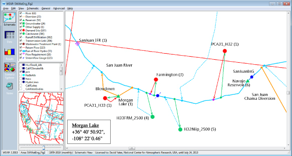
Figure 3. The WEAP-SW modeled, zoomed in over northwestern New Mexico and the San Juan River.
Download figure:
Standard image High-resolution image3. Model evaluation and results
Model calibration was performed using manual techniques targeting observed streamflow, snow water equivalent measurements, reservoir storage, water deliveries, and water use. Select sub-basins for model calibration and evaluation are shown in table 3. An initial set of parameters was developed that could be applied across all the watersheds, meant to capture the seasonal and inter-annual variability of river flow, snow, reservoir, and water use measurements across the southwest. The most sensitive model parameters were then adjusted on a regional, resulting in a unique set of parameters for the headwater basins of Colorado, New Mexico, Utah, and Wyoming (Upper Colorado); the southwestern Arizona Basins including the Salt and Gila Rivers, western Utah, and the Nevada basins (Southwestern); and the California Watersheds. The final set of calibrated model parameters included soil water capacity, hydraulic conductivity, melt and freeze temperatures, and preferred flow direction in order to account for differences in watershed characteristics not captured by the available data (table 4).
Table 4. Final set of model parameters applied to the WEAP-SW model by region. PFD—preferred flow direction (from 0.0, vertical to 1.0, horizontal); Kc—hydraulic conductivity (mm/month); RRF—runoff resistance factor. Smaller values of RRF lead to greater contribution from surface runoff.
| Parameter | Upper Colo | Southwest | California | |
|---|---|---|---|---|
| PFD | 0–2000 | 0.4 | 0.4 | 0.3 |
| 2000–3000 | 0.6 | 0.65 | 0.7 | |
| 3000–4000 | 0.8 | 0.7 | 0.8 | |
| Shallow soil Kc | Forest | 320 | 240 | 800 |
| Non-forest | 275 | 200 | 600 | |
| Urban | 150 | 125 | 300 | |
| Agriculture | 300 | 200 | 300 | |
| Shallow soil cap (mm) | Forest | 850 | 640 | 600 |
| Non-forest | 600 | 450 | 450 | |
| Urban | 300 | 300 | 300 | |
| Agriculture | 600 | 500 | 700 | |
| Surface RRF | Forest | 4 | 4 | 3 |
| Non-forest | 3 | 3 | 2 | |
| Urban | 1 | 1 | 1 | |
| Agriculture | 6 | 6 | 6 | |
| Deep soil Kc (mm/month) | 300 | 200 | 400 | |
| Deep soil capacity (mm) | 500 | 850 | 850 | |
| Melting (°C) | 7 | 5.5 | 3 | |
| Freezing (°C) | −3 | −5 | −5 | |
In addition to hydrologic parameters, the model includes characterization of reservoir operations through maximum release and diversion rates and infrastructure capacities, as the WEAP-SW endogenously models the large water diversions through the major water supply systems of the southwest. The majority of this infrastructure is managed by the US Bureau of Reclamation, and includes such projects as the Colorado Big Thompson, the Central Arizona Project, the Colorado Aqueduct, the All American Canal, the California State Water Project, the California Central Valley Project, and others.
The locations where model performance was evaluated are shown in figure 4. The accuracy of the model at simulating streamflow (figure 5), reservoir storage (figure 6), and snow water equivalent or SWE (figure 7) were quantified using goodness of fit statistics generally for the years 1980–2010 (n = 372 for monthly statistics; n = 31 for yearly statistics), with 1979 used as a model spin up year. In some cases, fewer years were used to match the available observations. Using streamflow as the interest field, where Qs,i and Qo,i are the simulated and observed monthly flow volumes at each time step (i), the statistics included.

Figure 4. Locations where summary statistics and plots of monthly and annual values are shown in figures 6, 7 and 8 for streamflow, reservoir storage, and snow water equivalent, respectively.
Download figure:
Standard image High-resolution image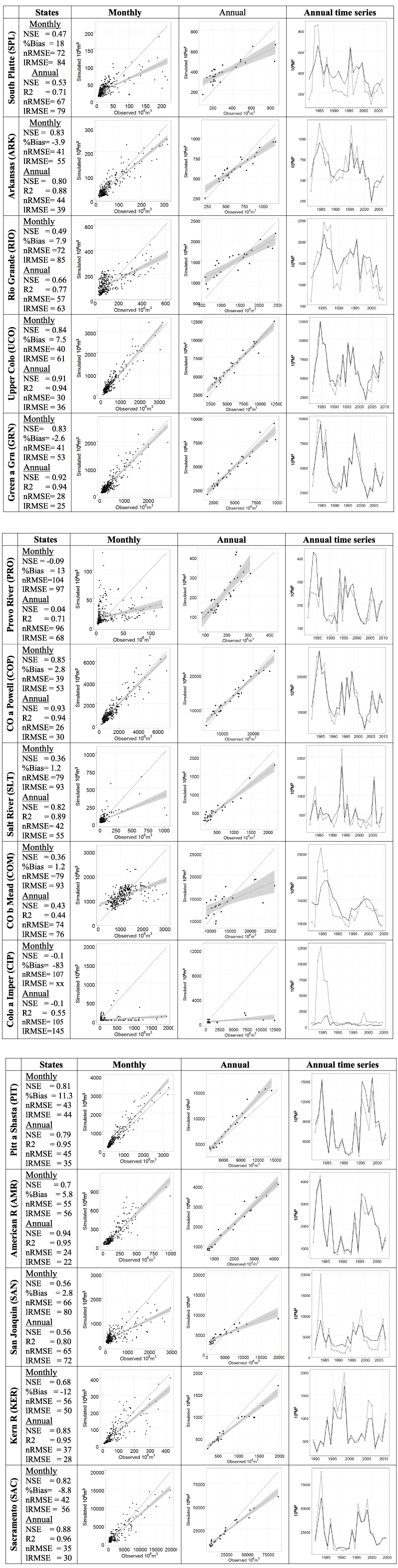
Figure 5. Simulated and observed streamflow at select locations across the southwestern US (see figure 3). Dark lines are the simulated values for annual series. NSE is Nash–Sutcliffe efficiency; nRMSE is the normalized root mean square error; and lRMSE is the log-transformed/normalized root mean square error.
Download figure:
Standard image High-resolution image
Figure 6. Simulated (dark line) and observed (light line) storage for four select reservoirs.
Download figure:
Standard image High-resolution image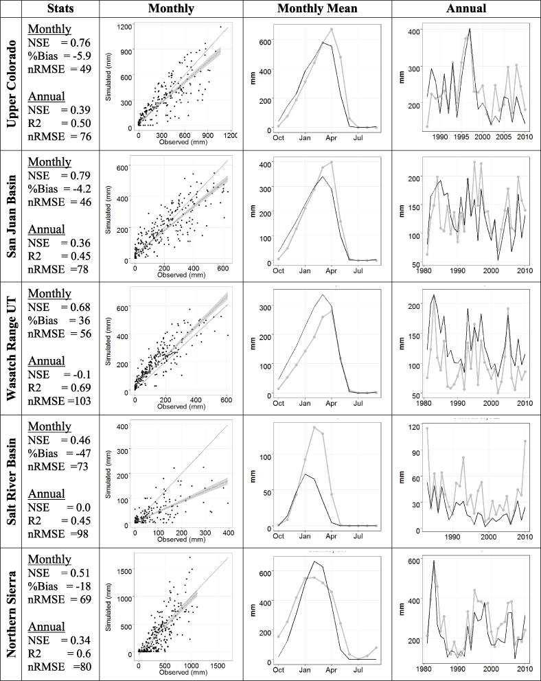
Figure 7. Summary of snow water equivalent (SWE), with simulated shown as the dark line and observed the light line for select locations.
Download figure:
Standard image High-resolution image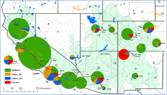
Figure 8. WEAP simulated annual average supply delivered to the four broad sectors, aggregated to the main use areas. The values near or within each red slice are the fraction of the supplied water that is consumed in thermoelectric generation. The numbers labeled 6–59 are the ReEDS PCA regions. Purple lines are the major diversions, and the orange lines are the irrigation systems.
Download figure:
Standard image High-resolution image
The Nash–Sutcliffe efficiency or  ; where a value of 1.0 is perfect match, a value of 0.0 indicates that the estimates area as good as the mean of the observed value while a value less than zero suggests that the observed mean is a better predictor than the estimate.
The per cent bias or ![$\mathrm{BIAS}=1 0 0[({\bar {Q}}_{\mathrm{s}}-{\bar {Q}}_{\mathrm{o}})/{\bar {Q}}_{\mathrm{o}}]$](https://content.cld.iop.org/journals/1748-9326/8/4/045004/revision1/erl465879ieqn25.gif) , which indicates if the model generally is over (positive) or under (negative) estimating the observed value; and the normalize root mean square error or
, which indicates if the model generally is over (positive) or under (negative) estimating the observed value; and the normalize root mean square error or  ; where σQo is the standard deviation of the observed flow volumes. A value 100% indicates that the estimate is the same magnitude as the variability of the flow. We also report the log of the nRMSE, given as lRMSE, where the non-zero flows have been log transformed to better evaluate low flow performance both seasonally and annually. Where a lRMSE value is lower than the nRMSE for a given watershed, suggests that the model is better at estimating low flows than high flows either on a monthly or annual basis. In addition, a correlation coefficient was calculated for some annual values and is reported in figure 5.
Overall the model captured the major features of the flow hydrographs of the watersheds presented in (figure 5). The WEAP-SW model showed less skill in simulating the smaller streamflows of heavily managed systems such as the South Platte River in Colorado and the Provo River in Utah. These statistics indicate a reduced goodness of fit when compared with the values at the larger river systems. Figure 5 shows that simulated flows for the South Platte Basin are biased high, but in terms of annual volume, are reasonable. The Arkansas River showed greater skill, particularly in the annual low flows, suggested by the lower lNRMSE compared with the nNRMSE.
The larger river systems tended to show closer agreement between observed and simulated values. For example, the simulated flows on the Colorado and Green Rivers that contribute to the largest storages in the southwest—Lake Powell and Lake Mead—showed good skill at both the monthly and annual levels, with monthly and annual nRMSE values of about 40% and 30%, respectively. Below Lake Mead, the resulting statistics largely reflect the ability of the WEAP-SW to characterize reservoir operations of Lake Powell and Lake Mead and the downstream demands including the Central Arizona Project, and water deliveries to California through the California Aqueduct and the All American Canal.
While the WEAP-SW includes the trans-basin diversions into these river systems, the diverted volumes are approximate and generally based on total annual volume accounting. For example, approximately 320 MM3 (260 000 acre-feet) of water is diverted annually from the Colorado River into the South Platte Basin via the Colorado Big Thompson project, but with considerable year-to-year variability in actual deliveries (USBR 2013). In the WEAP-SW model, water curtailments to these kinds of trans-basin systems are a function of the estimated adjudicated volume, demands on the system, and the associated demand priorities.
Table 5 shows the annual average delivery5 for the major water projects across the southwestern states, with WEAP-SW delivery estimates close to the total average annual estimate of 22 billion m3 (BCM), which is about 25% of the annual average reservoir storage in the region. The average total annual simulated water delivery was 75 (BCM), with groundwater making up 25 BCM on average. The minimum/maximum surface water delivery was 70/78 BCM (56.8/63.2 MAF), while the minimum/maximum groundwater delivery was 16/32 BCM (13/26 MAF). Annual average delivery for thermoelectric cooling, including once-through plants, was 5.2 BCM.
Table 5. Maximum, minimum and mean annual project water deliveries as estimated by WEAP-SW in million m3 compared with mean annual estimates from state records.
| Max | Min | Mean | State est. | |
|---|---|---|---|---|
| All American Canal, CA | 9 257 | 4 594 | 6 825 | 7 300 |
| Central Arizona Project, AZ | 2 274 | 775 | 1 470 | 1 800 |
| Central Valley Project, CA | 12 034 | 2 423 | 7 194 | 8 600 |
| Colorado Big Thompson, CO | 411 | 310 | 378 | 320 |
| Colorado Aqueduct, AZ&CA | 1 412 | 814 | 1 100 | 1 000 |
| Utah Project | 385 | 188 | 279 | 290 |
| Front Range Diversions, CO | 148 | 143 | 147 | 150 |
| Frying Pan-Arkansas Proj, CO | 166 | 55 | 112 | 150 |
| Hetch Hetchy, CA | 331 | 303 | 327 | 350 |
| Los Angeles Aqueduct, CA | 681 | 74 | 438 | 493 |
| State Water Project, CA | 3 944 | 1 713 | 2 836 | 3 100 |
| San Juan Chama Project, NM | 267 | 88 | 148 | 140 |
| Trinity Project, CA | 936 | 358 | 580 | 720 |
| Total | 32 246 | 11 838 | 21 832 | 24 400 |
Figure 6 shows simulated and observed reservoir storage for Lake Powell and Lake Mead, and suggests that the WEAP-SW model captured the general characteristics of reservoir fill and release dynamics over time. The WEAP-SW model overestimated the very low flows of the Colorado River below Imperial Reservoir, and missed the extreme high flow period of the early 1980s altogether, most notably the flood event of 1983. Figure 6 also shows two of the larger reservoirs in California, including Lake Shasta in the northern portion of the state and Millerton in the south San Joaquin. Relative to Lake Powell and Lake Mead, these reservoirs are small and thus exhibit much greater inter-annual variability, as the impact of wet and dry episodes are more pronounced. The WEAP-SW model captured this variability, with NSE suggesting fair to good agreement between simulated and observed monthly storage.
Figure 7 compares SWE for the select location in figure 4. The model shows generally good agreement between observed and simulated values, although interpolation of point observations of precipitation into spatially distributed fields useful for watershed modeling is a challenge. In the case of the Rocky Mountains and Sierra Nevada, it is especially difficult in the higher elevation catchments due to the lack of observational data and pronounced orographic effects. Previous efforts at modeling rainfall-runoff in the Sierra Nevada have encountered similar problems (McCabe and Clark 2005) and have adjusted the precipitation inputs to enable a better match between observed and simulated stream flow values (Koczot et al 2004).
4. Conclusion
A large-scale, climate drive water resources planning model of the southwestern US has been developed using the Water Evaluation and Planning (WEAP) decision support system. The model, referred to as WEAP-SW, simulates both managed and natural flows for the major river basins of the region, from the east slope watersheds of the South Platte and Arkansas Basins of the Colorado Rockies, to California's Sierra Nevada and Coastal Ranges of California, the WEAP-SW includes more than 35 BCM of surface storage, used to delivery around 75 BCM annually for municipal, industrial, agriculture, thermoelectric cooling, and environmental needs. The WEAP-SW model lends itself to the inclusion of the human intervention into the hydrologic cycle through reservoir and large-scale diversions for agriculture and municipal and industrial use including thermoelectric cooling. It is therefore a powerful tool to help evaluate climate change impacts and adaptation options for resource managers at the subwatershed scale, where water infrastructure such as thermoelectric cooling exists.
Acknowledgments
We gratefully acknowledge funding for this research from The Kresge Foundation, Wallace Research Foundation, and Roger and Vicki Sant, and the research oversight provided by the EW3 Scientific Advisory Committee—Peter Frumhoff (Union of Concerned Scientists), George Hornberger (Vanderbilt University), Robert Jackson (Duke University), Robin Newmark (NREL), Jonathan Overpeck (University of Arizona), Brad Udall (University of Colorado Boulder, NOAA Western Water Assessment), and Michael Webber (University of Texas at Austin). This research was also supported by the Societal Applications Research Program of the National Oceanic and Atmospheric Admiration's (NOAA) Climate Program Office (CPO) Grant NA10OAR4310186; and the Weather and Climate Assessment Program of the National Center for Atmospheric Research (NCAR). NCAR is a supported by the National Science Foundation.
Footnotes
- 5
We refer to delivery as the water take from a surface water or groundwater source and supplied to a demand. In most cases, there is a proportion returned to either a downstream demand or groundwater system. The difference between the delivered volume and the volume returned is the consumptive use.