
Abstract
Electric power generation often involves the use of water for power plant cooling and steam generation, which typically involves the release of cooling water to nearby rivers and lakes. The resulting thermal pollution may negatively impact the ecosystems of these water bodies. Water resource systems models enable the examination of the implications of alternative electric generation on regional water resources. This letter documents the development, calibration, and validation of a climate-driven water resource systems model of the Apalachicola–Chattahoochee–Flint, the Alabama–Coosa–Tallapoosa, and the Tombigbee River basins in the states of Georgia, Alabama, and Florida, in the southeastern US. The model represents different water users, including power plants, agricultural water users, and municipal users. The model takes into account local population, per-capita use estimates, and changes in population growth. The water resources planning model was calibrated and validated against the observed, managed flows through the river systems of the three basins. Flow calibration was performed on land cover, water capacity, and hydraulic conductivity of soil horizons; river water temperature calibration was performed on channel width and slope properties. Goodness-of-fit statistics indicate that under 1980–2010 levels of water use, the model robustly represents major features of monthly average streamflow and water temperatures. The application of this integrated electricity generation–water resources planning model can be used to explore alternative electric generation and water implications. The implementation of this model is explored in the companion paper of this focus issue (Yates et al 2013 Environ. Res. Lett. 8 035042).
Export citation and abstract BibTeX RIS

Content from this work may be used under the terms of the Creative Commons Attribution 3.0 licence. Any further distribution of this work must maintain attribution to the author(s) and the title of the work, journal citation and DOI.
1. Introduction
The power sector withdraws substantial cooling water for electricity generation across the US (Kenny et al 2009, Solley et al 1998). It is the single biggest user of water in the economy (Carter 2010) and is thus heavily dependent on available water resources. Consequently, any changes in water supply undermine the reliability of power generation. Understanding how electricity sector choices affect future water use is important (e.g. Roy et al 2012 and Elcock 2008). Power plant water use for cooling accounts for over 40% of freshwater withdrawals in the US, principally due to thermoelectric plants using once-through cooling (Stillwell et al 2011, Kenny et al 2009, Hutson et al 2004). Withdrawals can be substantially reduced by switching to evaporative or recirculating cooling, but the switch may increase overall consumptive use (Macknick et al 2012).
These connections between water use and energy production have resulted in a growing interest in integrated water–energy–climate analysis, especially for policy makers and planners. Recent studies in the arena of water–energy policy include: (1) three water–energy nexus cases in the United States through which a set of institutional relationships were studied with an emphasis on decision-making challenges faced by society (Scott et al 2011); and (2) a quantitative analysis, identification, and characterization of key actors and groups employing organization theory to bridge inter-organizational in order to develop a systematic and analytical approach for water and energy planning in Jordan (Siddiqi 2013).
In the southeastern US, climate change is projected to impact both natural and human systems (Christensen et al 2007). The Intergovernmental Panel on Climate Change (IPCC) in 2007 predicted that the southeast might experience increased climate variability, including more severe periods of drought coupled with wetter periods, as a result of climate change taking effect in North America (Christensen et al 2007). While the general implications of climate change on the hydrology of the southeastern US have caught policy makers' attention, there has been little region-wide analysis of the implications of future climate change on inter-connected water systems, with specific adaptive responses yet to materialize. Thus, it is important to understand the energy–water dynamics at present compared with the future. A larger fraction of freshwater withdrawals are for thermoelectric cooling in the southeast (75%) compared to the national portfolio (41%). This trend contributes to water supply stress in the region. However, in the southeast, problems related to water use for energy production are not confined to water quantity. Power generation typically involves the release of cooling water to nearby surface water resources (Averyt et al 2011), and the resulting thermal pollution negatively affects ecosystems. Thus, the role of water temperature and thermal pollution is important as well.
Water temperature problems for power plants most often arise during heat waves, when the temperature of intake water is elevated and electricity loads (largely for air conditioning) are high (Wilbanks et al 2008). Warmer water is less effective at cooling, making power plants uncompetitive and at times even causing power plants to temporarily shut down. Furthermore, rising water temperatures imperil fish and other aquatic species (Hester and Doyle 2011). A prime example in the southeastern US of power plant cooling water requirements and water demands interacting and adding stress to the system is an area of the Appaloosa–Chattahoochee River between Lake Lanier and West Point Reservoir. This area includes the Atlanta Metro Area, with a population about four million people and associated water withdrawals for urban consumption and cooling water for electricity generation from the Chattahoochee River. Changes in stream water temperature regimes are complicated by attenuation and cold-water releases from reservoirs like Lake Lanier, and return flows from thermoelectric cooling water and others uses, which are important to consider especially during the summer months and other times of low streamflow (USGCRP 2009).
To explore possible strategies for adaptation and management and the implications for water use by the energy sector, an analytical platform is needed that will allow for a better understanding of the climate change impacts within individual river basins. Such a platform allows us to assess how water and land managers may adapt to these impacts, since many management decisions are made at a local scale for individual basins (Yates and Miller 2013). As a case study in the exploration of flow and stream temperature issues, this study focused on the Apalachicola–Chattahoochee–Flint (ACF) basin and the Alabama–Coosa–Tallapoosa (ACT) basin. A model was developed to include a representation of the water resource and the water implications for energy production in these basins, with a particular focus on a few river reaches where with substantial cooling water used for thermoelectric generation. The model allows examination of instream water temperature, surface water availability, and different development pathways under current and future conditions. The case study considers current energy demands derived from the National Renewable Energy Laboratory (NREL) Regional Energy Deployment System (ReEDS) analysis that has been conducted independently for the entire United States (Clemmer et al 2012). Other development pathways are explored including projected changes in population growth and water demands from agriculture.
This letter presents the development of a southeastern US water systems model developed on the Water Evaluation and Planning (WEAP) system platform (Yates et al 2005). This model, hereafter called WEAP-SE was created to (1) represent the water supply and use of 44 hydrologic units (identified by a hydrologic unit code or HUC) in Alabama, Georgia, and Florida (figures 1 and 2) and the implications of hydrologic infrastructure such as reservoirs on the river's hydrology (flow and temperature); (2) describe the calibration of the WEAP-SE model to the managed flows of these river systems and how it is used to represent the water supply; and (3) to derive modeling results for stream temperature and subsequent thermal pollution effects on ecosystems. In the companion paper, we analyze some specific reaches where cooling water is used in thermoelectric generation, including the Chattahoochee River below Atlanta and above West Point Lake, with Plant Wansley and other thermoelectric cooling; and the Coosa River near the Georgia–Alabama River that includes once-through Plant Hammond and other large thermoelectric cooling facilities such as Plant Bowen. Plant Wansley and Plant Hammond are placed in figures 1 and 2.

Figure 1. The WEAP-SE domain, with the Apalachicola–Chattahoochee–Flint (ACF) basin in green and orange, Alabama–Coosa–Tallapoosa (ACT) basin in yellow, and the Tombigbee River basin in blue. ReEDS PCA regions (red) are labeled with the numbers 87–95. The region's rivers are in light blue.
Download figure:
Standard image High-resolution image
Figure 2. Location of the different streamflow gages used for model calibration in the Alabama–Coosa–Tallapoosa basin, Apalachicola–Chattahoochee–Flint basin, and Tombigbee River basin. ID numbers and abbreviations are listed in the table.
Download figure:
Standard image High-resolution imageAn application of the WEAP-SE model is performed by Yates et al (2013b) who investigate localized results by coupling the detailed model of geographically specific projections with both anthropogenic and natural aspects of the hydrologic systems of the ACF and ACT basins. Specifically, the study focuses on the two specific regions that include: Georgia Power's Plant Hammond, located in the Coosa River above Lake Weiss in the ACT basin and Georgia Power's Plant Wansley and other thermoelectric facilities in the Chattahoochee River above West Point Lake in the ACF basin (figures 1 and 2). Thermoelectric cooling technologies differ throughout the basins. For example, Plant Hammond, on the Georgia side of the border on the Coosa basin, is an 800 MW coal plant with once-through cooling. Just downstream is Lake Weiss, now a destination fishing lake that provides important tourism income for Cherokee County, AL (Glover 2012) but was originally impounded for hydroelectric power generation. On the Chattahoochee River, Plant Wansley is a 3939 MW power plant fueled by coal (44%), natural gas combined-cycle (55%), and oil (1%), cooled with recirculating cooling system. These different cooling technologies have different effects on the rivers of these basins, with Yates et al (2013b) examining both region-wide impacts on water resources and focused impacts on changes in water volume and temperature at these locations under current and project future region-wide electricity mix fuels (coal, natural gas, renewables, etc) and cooling technologies (once-through, recirculating, dry, etc).
2. Methodology: WEAP as an analytical framework
The WEAP decision support system (DSS) is a comprehensive, fully integrated water system simulation model that includes a robust and flexible representation of water demands from all sectors (Yates et al 2005). It allows for the description of operating rules for infrastructure elements such as reservoirs, diversions, environmental flows, canals, and hydropower (Sandoval-Solis and McKinney 2009, Thompson et al 2012). It has basin rainfall-runoff modeling capabilities that allow for the calculation of hydrograph components including runoff, interflow, and base flow (Yates et al 2005). Soil moisture storage and snow accumulation and melt are also calculated. Water infrastructure and demand elements can be dynamically nested within the underlying hydrological processes. In effect, this allows the modeler to analyze how specific configurations of infrastructure, operating rules, and priorities will affect different water uses, such as instream flows, agricultural irrigation, and municipal water supply under climate forcing and physical basin conditions (Yates and Miller 2013, Yates et al 2009). This makes it ideally suited to studies of dynamic change within basins, such as climate warming. In order to represent the water infrastructure and management of the Southeast's ACF and ACT systems, a DSS model was built for both basins and also for the adjacent Tombigbee River basin (figure 2).
The physical hydrology model in WEAP represents the terrestrial water cycle with a series of simultaneously solved equations. Rainfall is partitioned into snow, runoff, or infiltration depending on temperature, land cover, and soil moisture status. Moisture in the root zone is partitioned into evapotranspiration, interflow, deep percolation, or storage as a function of soil water capacity, hydraulic conductivity, potential evapotranspiration (ET), and vegetation-specific ET coefficients. Deep percolation enters a second soil compartment and is partitioned into base flow or deep soil moisture storage. This partitioning is a function of the soil moisture storage status, the water holding capacity of the deep compartment, and the hydraulic conductivity of the deep sediments. For a detailed discussion of the model algorithms see (Yates et al 2005). Due to the importance of stream temperature in southeastern hydrology, the water temperature model is described here. WEAP has a simple mixing model that computes a weighted average of the water temperatures based on the inflows from upstream, tributaries' return flows, and groundwater inflows (Yates et al 2005). The volume for a reach is defined by its length and average cross sectional area with an assumption of steady state in each time step where a heat balance equation is calculated for each reach on the river (equation (1)).
The terms on the right-hand side are:
 : upstream heat input to the stream segment with constant volume, with V (m3) expressed as a relationship of flow and Qi (m3/time) and temperature, Ti, at the upstream node.
 : net radiation input, Rn, to the control volume with density, ρ; Cp, the specific heat of water; and H(m), the mean water depth of the stream segment.
 : atmospheric long-wave radiation into the control volume, with the Stefan–Boltzmann constant (C; Tair, the air temperature; a, a coefficient to account for atmospheric attenuation and reflection; and the air vapor pressure, eair.
 : the heat leaving the control volume.
 : long-wave radiation of the water that leaves the control volume.
 ,
,  : the conduction of heat to the air and the removal of heat from the river due to evaporation. The terms f(u) and g(u) are wind functions, and D is the vapor pressure deficit. The temperature, Ti+1 is solved for the downstream node with a fourth-order Runge–Kutta method and is the boundary condition temperature for the next reach (after mixing of any other inflows into the downstream node is considered).
2.1. WEAP catchment delineation
Catchment nodes in WEAP were used to represent topographically identified sub-catchments that are characterized by unique climate, land cover–land use (LULC), and soil water properties (table 1). Climate forcing data are applied uniformly over each sub-basin area. The hydrologic model within each sub-catchment was parameterized using publicly available LULC classes from the National Land Cover Dataset (NLCD) (Homer et al 2004) (www.epa.gov/mrlc/nlcd-2006.html), and 30-m digital elevations from the National Hydrography Dataset-Plus (NHD Plus) (www.horizonsystems.com/NHDPlus/index.php). WEAP sub-catchment definitions were achieved using the following steps: (1) identification of the major southeastern rivers modeled in WEAP according to the basin and sub-basin designation of the US Geological Survey (USGS) HUC system (hereafter referred to as basins); (2) intersection of 500-m elevation bands within each basin to create WEAP sub-catchments; (3) classification of LULC within each sub-catchment according to LULC categories; (4) calculation of fractional areas for each LULC in each WEAP sub-catchment. See Yates et al (2013a) for further details in methodology.
Table 1. Sources of digital data used for building the WEAP-SE model.
| Model component | Use/assumption | Source |
|---|---|---|
| Rivers/tributaries, basin boundaries and contributing areas, and hydropower potential | General model development and hydrologic connectivity. Elevations used to determine hydropower potential | The National Hydrography Dataset-Plus (NHD Plus) (www.horizon-systems.com/NHDPlus/index.php) |
| Land cover categories: forested, non-forested, irrigated agriculture, and urban | Four-land classes are adequate to determine the hydrologic response of the catchment. Used to estimate irrigated acreage | The National Land Cover Dataset 2006 (www.epa.gov/mrlc/nlcd-2006.html) |
| Gridded climate forcing of monthly total precipitation and monthly average temperature | Climate forcing for each catchment object computed as the average of each catchment's elevation band | The Bias Corrected and Downscaled WCRP CMIP3a Climate and Hydrology Projection Archive (http://gdo-dcp.ucllnl.org) for historic and future climate data |
| Observed monthly average streamflow and water temperature | Used in model calibration | US Geological Survey for historic water data on streamflow, water quality, water demand, etc (http://water.usgs.gov/) |
| Reservoir capacities, head-area-volumes, dam height and tailwater elevations, turbine capacities, hydropower operating criteria | Specification of reservoir capacity and operating procedures. Determination of reservoir evaporative losses, conservation and flood control storage, and hydropower generation | US Army Corps of Engineers, for the ACF and ACT project specific information on water supplies, dams, water operations, hydroelectricity, etc (http://water.sam.usace.army.mil/default.htm |
| Water use: municipal, industrial and irrigated agriculture, thermoelectric generation and cooling. Per-capita water use. Local groundwater availability, attributes, and proportional use | Assumed constant per-capita water demand that represents a withdrawal with 50% consumption. Local groundwater attributes. WEAP supply priorities applied based on regional descriptions. Local data used to refine agricultural water use and hydropower production | State and local data resources—Georgia: Atlanta Department of Watershed Management; Alabama: Alabama Department of Environmental Management (www.atlantaga.gov/index.aspx?page=194; www.adem.state.al.us/default.cnt) |
aWorld Climate Research Programme (WCRP) Phase 3 of the Coupled Model Intercomparison Project (CMIP3).
Basin pour points were placed at important infrastructure including dams, diversions, return flow structures, and USGS streamflow gages, with a subset of those listed in table 2 and other gages placed internally to ensure adequate representation of streamflows during the model calibration process. These basin pour points were used as calibration points for reproducing streamflows and suitable water temperatures. These calibration points were distributed through the basins and in some key areas, such as the Atlanta Metro Area, the density of these calibration points is higher in order to accurately represent the current conditions of streamflow and water temperature. This delineation resulted in nine river objects or 'basins' in WEAP-SE. Each basin includes a collection of 44 sub-catchments with an average area of 3779 km2 (figure 1). LULC classes were aggregated into four categories including forested, non-forested, irrigated agriculture, and urban.
Table 2. Basin name and model information implemented in the WEAP-SE model (see figure 1).
| Basin name | Code | State | Basin point or outlet | No. of sub-catchments |
|---|---|---|---|---|
| Apalachicola_Chattahoochee | ACR | GA, AL, FL | Sumatra, FL 02359170 | 5 |
| Flint | FFL | GA | Newton, GA 02353000 | 6 |
| Chipola | CPL | FL | N/A | 1 |
| Coosawattee | CSW | GA | Rome, GA 02397000 | 3 |
| Coosa_Alabama | CAL | GA, AL | Monroeville, AL 02428400 | 9 |
| Tallapoosa | TLP | AL | Montgomery, AL 02420000 | 3 |
| Cahaba | CHB | AL | N/A | 1 |
| Black warrior | BLW | AL | Eutaw, AL 02466030 | 5 |
| Tombigbee | TBG | MS, AL | Coffeeville, AL 02469761 | 11 |
| Total number sub-catchments | 44 | |||
| Average area (±SD) | 3779 km2 (1539 km2) | |||
2.2. Water use, climate, and infrastructure data
The primary data inputs to the WEAP-SE model include time series of monthly climate; estimates of monthly water use including irrigated agriculture, urban (or municipal) and industrial, thermoelectric cooling, and environmental flows; and infrastructure elements including reservoirs, diversions, and their capacities, and regulated constraints (table 3). In this letter, values of water use estimates do not change over time and uncertainties are not considered. In the companion paper (Yates et al 2013b), uncertainties are included and analyzed.
Table 3. Regional population, agricultural areas, and water use by sector for the ACF and ACT basins. Municipal and Industrial (M&I) indoor per-capita rates are 473 l per day (LPD) (125 gallons per day (GPD)).
| Region (population)a | Agriculture (km2) | M&I (Mm3) | Agriculture (Mm3) | |
|---|---|---|---|---|
| Alabama | Mid Alabama (571) | 950 | 97.2 | 397 |
| Tallapoosa (381) | NA | 65.7 | NA | |
| Montgomery metro area (325) | NA | 56.2 | NA | |
| Alabama (338) | NA | 58.3 | NA | |
| Low Alabama (404) | NA | 69.8 | NA | |
| Georgia | Upper Chattahoochee (0.26) | 314 | 0.04 | 218 |
| Metro Atlanta (4000) | NA | 690.6 | NA | |
| Upstream west point (310) | NA | 53.5 | NA | |
| Upper flint (148) | 960 | 25.6 | 465 | |
| Flint (478) | 3755 | 82.5 | 1688 | |
| Low Chattahoochee (528) | 3171 | 91.2 | 1650 | |
| Florida | Apalachicola–Chattahoochee (195) | 1648 | 33.7 | 547 |
| Total | (7678) | 10 798 | 1326 | 4965 |
aPopulation (×1000) in the year 2000 and corresponding level of indoor and agriculture water use or delivered water.
A bias corrected and downscaled World Climate Research Programme (WCRP) CMIP3 (Phase 3 of the Coupled Model Intercomparison Project) Climate and Hydrology Projection Archive supplied climate data; gridded climate forcing for each catchment object was computed based on the average of each catchment's elevation bands (table 1). A gridded dataset for the continental US was chosen for this application due to its spatial resolution (∼12 km grid), which is fine enough to provide resolved temperature and precipitation values for sub-catchments that may be close in proximity but at different elevations (Maurer et al 2010). From the gridded data, monthly total precipitation and mean temperature were spatially averaged for each sub-catchment for the period 1949–2010.
Water allocation in WEAP is established through a set of user-defined demand priorities and supply preferences that are used to construct an optimization routine that allocates available supplies at each time step. A linear programming (LP) algorithm allocates water to maximize satisfaction of demand, subject to supply priorities; demand site preferences; mass balance; and other constraints (Yates et al 2005). Demands, reservoir storage, hydropower, and instream flow requirements are assigned a unique integer priority number, ranging from 1 (the highest priority) to 99 (the lowest priority). Those entities with a priority 1 ranking are members of Equity Group 1, those with a priority 2 ranking are members of Equity Group 2, and so on. The LP constraint set is written to supply an equal percentage of water to the members of each equity group. The priority numbers are not weights, but ensure that demands with priority 1 are allocated water before those with priority 2, priority 2 before priority 3, and so on. In the WEAP-SE model, the priority ranking is given as: priority 1: instream flow requirements; priority 2: urban indoor water and thermoelectric cooling; priority 3: irrigated agriculture; and priority 4: reservoir filling. This ranking means that other uses will be curtailed to meet instream flow and thermoelectric cooling water requirements under water-constrained conditions.
Water use was estimated for each sector in the corresponding monthly time step, primarily from different publicly available sources (table 1). Municipal, commercial, and industrial indoor uses (excluding thermoelectric generation) were based on estimates of population and liters-per-capita-per-day or LPD (gallons-per-capita-per-day or GPD). A value of 473 LPD (125 GPD) for residential use includes 95 LPD (25 GPD) for commercial and industrial use.
For streamflow and water temperature data USGS and US Army Corps of Engineers (USACE) streamflow gages were used to obtain pertinent information on a monthly average time step for continuous record data. The ACF and ACT USACE projects provided infrastructure-related data such as reservoir capacity, head-volume, dam heights and tailwater elevations, turbine capacities, and historic hydropower generation data (table 1).
Irrigated agricultural use was based on the general agricultural practices and irrigated acreage in the southeast region and made use of WEAP's internal soil moisture deficit model to trigger a monthly irrigation application. Irrigated agriculture was active in twelve of the 44 sub-catchments, with a total irrigated area of 320 km2 (79 thousand acres). In each catchment object that included irrigation, a representative irrigation schedule was used to approximate general irrigation practices in the region (irrigation was scheduled to happen from April to September). A specific cotton category was included in the lower ACF's catchment objects. Cotton is an important commodity and is the most demanding crop from the point of view of water consumption in the region, with an irrigation schedule happening from June to August. We have identified general irrigated acreage and crop type to estimate annual applied water. The average annual applied irrigation depth is 800 mm (31.5 in) in the ACF basin. A simple representation of a surficial aquifer in the lower ACF basin that feeds mainly the irrigated agricultural areas was also implemented in the WEAP-SE model as a groundwater source. The aquifer's representation in WEAP was a simplification of the groundwater system as a reservoir with a storage capacity of 1400 Mm3, hydraulic conductivity of 30 m per day, and a specific yield of 0.08.
The focus on thermoelectric generation and associated cooling water warrants special attention (see (Sattler et al 2012). ReEDS models electric generation and capacity by generation technology at the level of the continental US's 134 power control authorities (PCAs) for a series of two-year periods between 2010 and 2050 (Short et al 2011). In this letter, the 2010 generation level was used to estimate thermoelectric water withdrawals and consumptive use for the WEAP-SE calibration period of 1980–2010. We used Macknick et al's (2012) work on a meta-analysis of published studies of cooling water use based on fuel type and cooling technology to provide water withdrawal and consumption coefficients to calculate water use for the WEAP-SE model. For each thermoelectric fossil fuel or nuclear generating technology represented in ReEDS, the generation and capacity data for each PCA is mapped to the HUC-8 region in an amount proportional to the capacity and generation determined by thermoelectric plant location as described in Averyt et al (2013). We then project plant locations onto the sub-catchment locations of individual plants throughout the WEAP-SE model.
3. Model calibration results
Model calibration was accomplished using manual calibration techniques targeting monthly values of observed streamflows, reservoir storages, water deliveries, and water use from several sources including the USGS and USACE gaging stations, and local, state, and federal databases and reports. Streamflow and water temperature data records were not continuous and did not cover the same period of time; consequently gaps were observed. Since the whole study area has similar physiographic conditions (e.g. altitude varied from 0 to 1000 m above sea level in a total area of 166 000 km2), an initial set of calibrating parameters was developed that could be applied across all nine sub-basins and capture the seasonal and interannual variability of flow measurements across the ACF, ACT, and Tombigbee basins (table 4). The most sensitive model parameters were then adjusted on a basin-by-basin basis, including soil water capacity and hydraulic conductivity for both shallow and deep layers (table 4) in order to account for fine-scale differences in basin characteristics not captured by the available data. The model uses the Penman–Monteith method (Monteith 1965) to estimate potential evapotranspiration and simulate soil water evaporation as a function of relative soil moisture.
Table 4. Parameters used on the WEAP-SE model. (Note: PFD—preferred flow direction (from 0.0, vertical to 1.0, horizontal); SSC—shallow soil capacity in mm; K—hydraulic conductivity (mm/month); SV—single value, not distributed by land class; RRF—runoff resistance factor—smaller values of RRF lead to greater component of surface runoff.)
| Parameters | Value | |
|---|---|---|
| PFD | 0–500 of SSC | 0.7 |
| 500–1000 of SSC | 0.6 | |
| Shallow soil Kc | Forest | 0–500 |
| Non-forest | 0–300 | |
| Urban | 80 | |
| Agriculture | 100 | |
| Shallow soil cap (mm) | Forest | 525–900 |
| Non-forest | 420–720 | |
| Urban | 500 | |
| Agriculture | 560–960 | |
| Surface RRF | Forest | 3 |
| Non-forest | 2 | |
| Urban | 1 | |
| Agriculture | 4 | |
| Deep soil Kc (mm/mo) | 100–125 | |
| Deep soil capacity (mm) | 600–1125 | |
| Crop coefficient, Kc | Jan–Apr: 1, May: 1.1, Jun–Aug: 1.2, Sep: 1.1, Oct–Dec: 1 | |
The accuracy of the model at simulating streamflow (figure 3), and temperature (figure 4) were quantified using goodness-of-fit statistics for the years 1980–2010 (n = 372 for monthly statistics). These included:

where a value of 1.0 is a perfect match, a value of 0.0 indicates that the estimates are as good as the mean of the observed value, and a value less than zero suggests that the observed mean is a better predictor than the estimate.

This indicates if the model generally is over- (positive) or under- (negative) estimating the observed value.

where nRMSE is the normalized root mean square error, Qs,i and Qo,i were the simulated and observed flow rates for each time step (i), and σQo is the standard deviation of the observed flows. A value of 100% indicates that the estimate is the same magnitude as the variability of the flow. The lRMSE (log-transformed/normalized root mean square error) is the same as nRMSE, except the non-zero flows have been log transformed to better evaluate low flow performance especially during low summer flows that have an ecological importance. In addition, the coefficient of determination, R2, was calculated for monthly values as well.
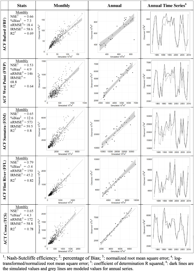
Figure 3. Monthly and annual simulated and estimated full natural flows with goodness-of-fit statistics at sub-basin outlets. The solid, dark line represents the 1:1 correspondence.
Download figure:
Standard image High-resolution image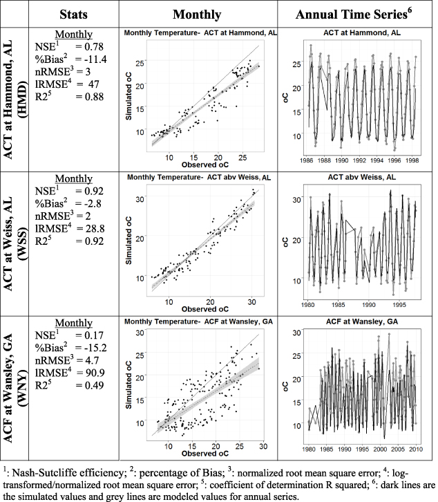
Figure 4. Monthly simulated and estimated streamflow temperatures with goodness-of-fit statistics at three locations of interest in the system. The solid, dark line represents the 1:1 correspondence.
Download figure:
Standard image High-resolution image
For streamflow, calibration was performed and values of the Bias ranged from −3.4% to 12.6% with an average of −5.1% (figure 3). The nRMSE varied from 18% to 573% with an average of 212%. These nRMSE values are widely spread mainly because the observed streamflow variability at Sumatra, FL. This condition improves when the lRMSE is evaluated. Values of lRMSE varied from 45% to 69% with an average of 58%. Similarly values of R2 ranged from 0.64 to 0.82 with an average of 0.75. Values of NSE ranged from 0.53 to 0.79 with an average of 0.66 indicating that the model robustly represents major features of monthly average steamflows. Overall, the model captured the major features of the flow hydrographs (figure 3) at the different basin outlets and accurately represents the low summer flows.
To assess model accuracy within the boundaries of the basins, flows from the USGS gage that measure runoff from an undeveloped sub-basin, the FBF (ACF above Buford, GA) on figure 3, represent unaltered conditions. These were compared to model predictions, resulting in a NSE value of 0.66, and Bias value of 7.3%. he nRMSE value was 18.4%, and the lRMSE value was 58.6%. These statistics indicate an acceptable goodness-of-fit for an undeveloped sub-basin when compared with the values at the gage location before streamflows enter Buford Dam (figure 3) in the upper Apalachicola–Chattahoochee basin.
A potential source of parameter specification error was identified during the model construction process. The STATSGO database (table 1), which uses soil surveys to characterize soils as either deep or shallow, had an average mapping unit polygon size of 126 km2, 30 times smaller than the average catchment size. Since the entire mapping unit was classified as shallow if one component had a measured bedrock depth less than 50 cm or was a rock outcrop, an overestimation of the shallow soil extent was likely.
Stream temperatures at different locations were also calculated and evaluated. Temperature calibration, similar to streamflow calibration, was based on comparisons between the different unimpaired and computed temperatures using the same statistical parameters (figure 4). Values of NSE ranged from 0.17 to 0.92 with an average of 0.62. The bias ranged from −15.2% to −2.8% with an average of −9.8%. Values of nRMSE varied from 2% to 4.7% with an average of 3.2%. Similarly, values of nRMSE were from 28.8% to 90.9% with an average of 55.6% (figure 4) and values of R2 ranged from 0.49 to 0.92 with an average of 0.76. Flow temperatures were captured well by the model especially during summer when there is a higher risk of having negative thermal pollution impacts (figure 4). One exception was the HMD location upstream of the Hammond Power Plant. At the WSS location downstream from the Hammond Power Plant, where water is discharged back into the stream after being used for cooling purposes, the temperatures robustly represent the monthly streamflow temperatures even during the warm season (figure 4). A similar condition is observed for the WNY location. Overall, the model captured the major trends of stream temperature (figure 4) and is an acceptable representation of summer flow temperature.
Users of this model should consider the calibration results outlined above in determining how to apply the model. Depending on the question to be addressed by the model, there are varying levels of confidence in its accuracy. Overall, the calibration results indicate that the model is accurate at predicting streamflows and temperatures, and therefore useful for exploring the implications of alternative electricity generation technologies, which is the subject of the companion paper (Yates et al 2013b).
4. Conclusions
Development and implementation of a climate-driven model for the ACF, ACT, and Tombigbee river basins in the southeastern US was accomplished to represent the different users of the water resources of the region systems and the implications of energy production on the riverine hydrology and water temperature regimes.
The primary data inputs include time series of monthly climate data; estimates of monthly water use including irrigated agriculture, municipal (and industrial) indoor use based on local population and per capita use estimates with changes in population growth, thermoelectric cooling demands, and environmental flows; and infrastructure elements including reservoirs, diversions, and their capacities and regulated constraints. The water resources planning model was calibrated and validated against the observed, managed flows through the river systems in the three basins. Basin pour points were placed at important infrastructure locations including dams, diversions, return flow structures, USGS streamflow gages, and other gages placed internally to secure the adequate reproduction of streamflows. Calibration was performed on parameters of land cover, water capacity, and hydraulic conductivity of soil horizons. Goodness-of-fit statistics indicate that the model robustly represents major features of monthly average streamflow and reservoir storage under 1980–2010 levels of water use.
Water temperatures were captured sufficiently well by the model especially during summer months when there is a higher risk of having negative thermal pollution impacts. Thermoelectric plants, which sit higher up in their respective watershed, are likely prone to generating constraints, either in the form of thermal discharge limits or water volume limits. For two places in which this analysis focuses, the plant Hammond, a once-through cooling, is flagrant, and at plant Wansley changes are rapidly occurring in the way thermoelectric plants use water. Analysis also shows that an alternative, low-carbon technologies would improve the water quality by lowering the river temperatures. Other way for improving negative thermal impacts is through reservoir releases that, however, would reduce the water storage capacity in reservoirs for other uses located upstream including municipal, industrial and irrigation. The model provides the tools to analyze climate change—induced alterations in the hydrologic cycle with a special emphasis on implications for energy production.
Acknowledgments
We gratefully acknowledge funding for this research from The Kresge Foundation, Wallace Research Foundation, and Roger and Vicki Sant, and the research oversight provided by the EW3 Scientific Advisory Committee—Peter Frumhoff (Union of Concerned Scientists), George Hornberger (Vanderbilt University), Robert Jackson (Duke University), Robin Newmark (NREL), Jonathan Overpeck (University of Arizona), Brad Udall (University of Colorado Boulder, NOAA Western Water Assessment), Michael Webber (University of Texas at Austin), and Todd Rasmussen (University of Georgia). This research was also supported by the Societal Applications Research Program of the National Oceanic and Atmospheric Admiration's (NOAA) Climate Program Office (CPO) Grant NA10OAR4310186; and the Weather and Climate Assessment Program of the National Center for Atmospheric Research (NCAR). NCAR is supported by the National Science Foundation.