

Abstract
This modelling study demonstrates at what level of global mean temperature rise (ΔTg) regions will be exposed to significant decreases of freshwater availability and changes to terrestrial ecosystems. Projections are based on a new, consistent set of 152 climate scenarios (eight ΔTg trajectories reaching 1.5–5 ° C above pre-industrial levels by 2100, each scaled with spatial patterns from 19 general circulation models). The results suggest that already at a ΔTg of 2 ° C and mainly in the subtropics, higher water scarcity would occur in >50% out of the 19 climate scenarios. Substantial biogeochemical and vegetation structural changes would also occur at 2 ° C, but mainly in subpolar and semiarid ecosystems. Other regions would be affected at higher ΔTg levels, with lower intensity or with lower confidence. In total, mean global warming levels of 2 ° C, 3.5 ° C and 5 ° C are simulated to expose an additional 8%, 11% and 13% of the world population to new or aggravated water scarcity, respectively, with >50% confidence (while ∼1.3 billion people already live in water-scarce regions). Concurrently, substantial habitat transformations would occur in biogeographic regions that contain 1% (in zones affected at 2 ° C), 10% (3.5 ° C) and 74% (5 ° C) of present endemism-weighted vascular plant species, respectively. The results suggest nonlinear growth of impacts along with ΔTg and highlight regional disparities in impact magnitudes and critical ΔTg levels.
Export citation and abstract BibTeX RIS

Content from this work may be used under the terms of the Creative Commons Attribution 3.0 licence. Any further distribution of this work must maintain attribution to the author(s) and the title of the work, journal citation and DOI.
1. Introduction
Countries' current pledges to reduce greenhouse gas emissions would set global mean temperature increase (ΔTg) on a trajectory of ∼3.5 ° C above pre-industrial levels by the end of this century (Rogelj et al 2010)—far above the 2 ° C target adopted in the Cancún Agreements (UNFCCC 2011). The tensions about the climate policy goal of limiting ΔTg to 2 ° C require that policymakers be informed about possible consequences of their decisions. This can be accomplished by solid scientific assessments of the presumably high costs, the implementation risks and the benefits (in terms of avoided climate change impacts) of low-stabilization targets on the one hand and of consequences of less ambitious mitigation (i.e. global warming above 2 ° C) on the other hand (Knopf et al 2012). To contribute to a better understanding of the latter, this study quantifies—spatially explicitly at global scale—how freshwater availability and terrestrial ecosystems might change in response to different levels of ΔTg.
Previous assessments of (exposure to) impacts associated with different ΔTg levels were compromised by a number of methodological inconsistencies, as pointed out e.g. by Lenton (2011) and Warren et al (2011). 'Reasons for concern' (Smith et al 2009) and 'burning ember' diagrams (Schneider and Mastrandrea 2005) often combine heterogeneous, partly qualitative impact estimates that lack spatial and temporal detail and do not systematically account for available climate change scenarios. Simulation models or other internally consistent balancing schemes, applied for the whole land surface and forced by simulations from a large ensemble of general circulation models (GCMs), can in principle overcome these inconsistencies. However, respective studies either focused on single, though politically relevant ΔTg levels (Fung et al 2010, Zelazowski et al 2011) or could not consider the structural uncertainty among GCMs—which is sizeable due to the large spread especially in precipitation projections (e.g. Knutti and Sedláček 2012). Often projections from only a few GCMs were used (Arnell et al 2011) or ensemble projections were grouped according to the warming level reached by the end of this century (Scholze et al 2006), which strongly reduces the sample size for higher ΔTg levels due to differences in the GCMs' climate sensitivity (see Rogelj et al 2012). Other studies (Tang and Lettenmaier 2012) selected those future time periods when a given ΔTg value was exceeded, which means that the timing of the Tg changes differed among GCMs. Yet other studies only investigated when and where specific temperatures or warming rates are likely to be reached, without quantifying resulting impacts (Joshi et al 2011, Mahlstein et al 2013).
To overcome many of these problems, we here employ a newly generated ensemble of 152 climate scenarios (Heinke et al 2012), constructed by performing a 'pattern-scaling' of stylized ΔTg trajectories (reaching 1.5–5 ° C above pre-industrial levels around year 2100, in 0.5° steps) with 19 GCMs from the CMIP3 archive. Used as forcing for the well-validated LPJmL biosphere and water balance model (Sitch et al 2003, Gerten et al 2004, Bondeau et al 2007), this setup enables consistent quantification of impacts for different ΔTg levels and underlying climate policies, respectively. The local–global scaling factors are nearly independent of the considered emissions scenarios and are sufficiently accurate over a wide range of ΔTg, especially in case of temperature but less so in case of precipitation (Mitchell 2003; see Heinke et al 2012 for details on this approach).
We present our results acknowledging that climate change proceeds asynchronously across the globe (i.e. some regions are affected earlier by significant changes than others; Joshi et al 2011, Mahlstein et al 2011) and that regions differ with respect to their vulnerability to such change (Füssel 2010). In so doing, we highlight which regions are likely to experience the here considered critical changes to water availability and ecosystems 'earlier' (i.e. at lower ΔTg levels around 2100) than others. To communicate these spatiotemporal patterns of exposure—and of implied global inequalities—we directly map the ΔTg level at which the local impacts on water and ecosystems first occur. We also demonstrate the incremental changes between different ΔTg levels.
2. Methods
2.1. Climate scenarios
We rearranged pre-existing GCM simulations using a pattern-scaling approach to allow for analysis of impacts under different levels of ΔTg while accounting for differences among GCMs. The principle of pattern-scaling is to calculate scaling coefficients that statistically link local changes in climate variables to ΔTg, global fields of which can be used in spatially resolved impact models.
The scaling coefficients were derived for each calendar month, for each grid cell over land (0.5° × 0.5° spatial resolution), and for each of 19 GCMs that participated in the World Climate Research Programme's Coupled Model Intercomparison Project (CMIP3) (Meehl et al 2007) to account for the large differences in GCM projections (see e.g. Knutti et al 2010). For each GCM and month, this procedure yielded the local change in climate variables (air temperature, precipitation amount, degree of cloudiness) per degree of ΔTg. These response patterns were then combined with time series of annual ΔTg derived from the reduced-complexity climate model MAGICC6 (Meinshausen et al 2011). Greenhouse gas emissions were tuned in MAGICC6 in a way that ΔTg levels of 1.5, 2.0, 2.5, 3.0, 3.5, 4.0, 4.5 and 5 ° C above pre-industrial levels (from the GCMs' unforced control runs) are reached by around year 2100 (2086–2115 average). Corresponding atmospheric CO2 concentrations range between ∼400 ppm (for the 1.5 ° C trajectory) and ∼1400 ppm (for the 5 ° C trajectory). As a result of this data fusion, 19 climate change patterns were obtained for each ΔTg step—152 scenarios altogether. The patterns were applied as anomalies to 1980–2009 observed climate (CRU TS3.1 for temperature and cloudiness, Mitchell and Jones 2005; and GPCC dataset versus 5 for precipitation, Rudolf et al 2010), yielding the 152 monthly time series up to year 2115. These data were subsequently interpolated to daily values using stochastic procedures as in Gerten et al (2004) and then used to force the LPJmL model for assessing potential impacts (see following sections). A comprehensive description of the generation of the scaling patterns and of the anomaly approach is provided by Heinke et al (2012). While biases in GCM projections have been accounted for in this data processing, we recognize that the skill of GCMs to project climate changes at regional scale is limited, as has been shown in a number of studies for CMIP3 models (e.g. Pincus et al 2008, Hawkins and Sutton 2010). Thus, the present scenarios are suited to identify the broad patterns of climate changes and their impacts (presented in global- and continental-scale plots and tables), but results for individual grid cells (presented in maps) should be interpreted with caution.
2.2. The LPJmL model
For quantifying the below-specified changes to water availability and ecosystems for each climate scenario, we employed the process-based LPJmL dynamic global vegetation and water balance model (Sitch et al 2003, Gerten et al 2004; with recent overall improvements by Bondeau et al 2007 and Rost et al 2008 but with crop, irrigation and river routing modules switched off—see section 2.3.1). LPJmL computes the growth and productivity of the world's major vegetation types (here, nine plant functional types) in direct coupling with associated fluxes of water and carbon in the vegetation–soil system. The model was run at daily time step and 0.5° × 0.5° spatial resolution globally, forced by the pattern-scaled time series of daily climate (air temperature, precipitation amount, number of wet days per month, cloud cover) and yearly atmospheric CO2 concentration. The model has been shown to well reproduce observed vegetation distribution, biomass production and carbon fluxes (Lucht et al 2002, Sitch et al 2003, Hickler et al 2006, Bondeau et al 2007), fire regimes (Thonicke et al 2001) and water fluxes (Gerten et al 2004, Rost et al 2008, Fader et al 2010). Hence, although individual process representations require continuous improvement in this model and others of its type (e.g. Sitch et al 2008, Li et al 2012, Murray et al 2013, Piao et al 2013), LPJmL is a suited tool for assessing climate change effects on water resources and ecosystems alike.
2.3. Change metrics
We consider local changes in water availability/scarcity and terrestrial ecosystems as expressed by two metrics, and subsequently relate these changes to the in situ human population size and 'species endemism' of vascular plants, respectively (see following paragraphs). The metrics are calculated for each 0.5° grid cell, ΔTg step and GCM pattern. The global warming level deemed critical from a local perspective is given by the lowest ΔTg value at which the metrics cross specific thresholds in the 2086–2115 average. We focus on changes projected to be 'more likely than not' (found in >50%, i.e. at least 10 out of the 19 climate change scenarios) but also address 'likely' (>66%) and 'unlikely' (<33% but >0%) impacts, following IPCC guidance notes (Mastrandrea et al 2010). We also focus on three policy-relevant ΔTg levels: the 2 ° C mitigation target; the likely outcome of current national emissions reduction pledges (3.5 ° C); and a business-as-usual case (5 ° C, near to the average ΔTg simulated by GCMs under high-emission SRES A1FI and RCP8.5 scenarios; Rogelj et al 2012). Since there are interdependencies among GCMs (Masson and Knutti 2011, Pennell and Reichler 2011), actual confidence may be narrower than stated herein. Moreover, although we have integrated all GCM runs with different initial conditions available from the CMIP3 archive (see Heinke et al 2012), they embody only a fraction of possible climate developments in the future (Rowlands et al 2012).
2.3.1. Water scarcity.
Chronic supply-side water scarcity—likely to increase competition among water users and to constrain food production, economic development and environmental integrity—is defined to prevail if <1000 m3 cap−1 yr−1 are available within a given spatial unit (Falkenmark and Widstrand 1992). This analysis uses river basins as the spatial unit, delineated as in Haddeland et al (2011), which implicitly assumes that any water demand is to be met within each basin, neglecting e.g. import of water-intensive products from other regions (Fader et al 2011). Furthermore, we consider only 'blue' water resources, i.e. renewable surface and subsurface runoff useable for irrigation, industries and households. Applying more complex water scarcity indicators and of other mapping units may yield different results (Gerten et al 2011). Runoff was computed under conditions of potential natural vegetation, for reasons of consistency with the assessment for ecosystems; irrigation, reservoir operation and land use change effects are thus not considered in this study. We distinguish four types of change to water resources and scarcity.
(1) Regions already chronically water-scarce experience aggravated scarcity. This is the case if the simulated annual and/or monthly runoff is significantly lower in the future (2086–2115 period) than presently (1980–2009). A significant decrease in the average annual runoff is assumed if its change is greater than present standard deviation (Gosling et al 2010, Arnell et al 2011), which can be regarded as a challenge to water management systems attuned to historic flow experience. A significant decrease in monthly runoff—taken as a proxy for increased drought frequency on top of the change in mean annual flow (Lehner et al 2006)—is assumed if the median of calendar months in the future is lower than the respective present-time median in more than 10% (i.e. 36) of the future months.
(2) Regions not yet chronically water-scarce move into a water-scarce status—i.e. <1000 m3 cap−1 yr−1 are simulated to be available in the future in regions that are above this threshold today.
(3) Regions not chronically water-scarce experience lower water availability. In this case the decrease in water availability is defined as in (1), yet applied to regions with >1000 m3 cap−1 yr−1 both presently and in the future.
(4) Regions that are water-scarce but do not experience aggravated scarcity; i.e. regions where present water availability is <1000 m3 cap−1 yr−1 but does not cross the thresholds cf case (1). Human populations are either held constant at year 2000 values or assumed to change according to the SRES B1 or A2r population projections, respectively (Grübler et al 2007). Increases in runoff are also analysed, but for reasons of brevity we do not relate them to the number of people living in areas affected by such increases.
2.3.2. Ecosystem change.
Severe ecosystem changes are assumed if the change in a generic ecosystem stability index 'Γ' developed by Heyder et al (2011) adopts a value ≥0.3 (moderate changes, Γ > 0.1). This can be interpreted as simultaneous shifts in several ecosystem features as large as those associated with e.g. a transition from temperate forest to boreal forest. The Γ metric is composed of a suite of biogeochemical and vegetation structural variables, changes in which either represent alterations in the entire ecosystem status or in a specific subset of variables. Using such an aggregated index advances earlier studies focused solely on biome area changes (Leemans and Eickhout 2004) or individual ecosystem properties (Gerber et al 2004, Scholze et al 2006, Sitch et al 2008).
Specifically, Γ encompasses the following components: (1) carbon fluxes (net primary production, heterotrophic soil respiration, carbon release from natural fires), (2) water fluxes (runoff, evaporation, transpiration), (3) carbon stocks (in plants and soils), and (4) vegetation composition ('ΔV' metric measuring structural dissimilarity of ecosystems based on life forms (trees, grass, bare ground) and their leaf architecture and phenology (needle-leaved or broadleaved, evergreen or deciduous; Sykes et al 1999)). Γ combines relative and absolute changes in these variables as well as changes in the proportional relation of carbon and water fluxes to each other. Some components are also scaled according to their signal-to-noise ratio. The overall Γ metric is finally normalized to values between 0.0 meaning no change and 1.0 meaning total restructuring of the considered basic ecosystem features. It was calculated for the uncultivated fraction of grid cells, thus maps and aggregated global values refer to the respective fractions of grid cells only. For a complete description of Γ see Heyder et al (2011), and also Ostberg et al (2013) who analyse it in more detail for the same climate scenarios as used here.
While Γ can be interpreted as overall habitat changes, the simulations do not contain information at species level. To frame the model results in the context of floral biodiversity (rather than merely counting the total area affected by Γ > 0.3 or >0.1 as in Ostberg et al 2013), we linked them to an independent global dataset of vascular plant (ferns, gymnosperms, angiosperms) biodiversity (Kier et al 2009). The dataset contains information on the current fractional distribution, species richness and endemism for each of 90 unique terrestrial (island and mainland) biogeographic regions—315 903 species altogether. The here used 'endemism richness' is the weighted product of the number of species within a biogeographic region and the region's share (0–1) of each species' global distribution range. For example, if 20% of a species' distribution range falls into a region, 20% of the total species number is attributed to it.
We determined, for each ΔTg step, which biogeographic regions experience changes in Γ on more than a third of their respective area, and counted how many of the 19 climate scenarios show this. We then determined the endemism richness of each of those regions from the Kier et al (2009) dataset, and aggregated the values to continental and global sums. Note that endemism richness refers to the present situation, whilst climatic and land cover changes may concurrently alter species richness and endemism (Sommer et al 2010). That is, our results do not indicate the climate effects on future endemism richness; they rather indicate the changing biogeochemical boundary conditions.
3. Results
3.1. Aggravation or new establishment of water scarcity
Figure 1 illustrates that certain regions are affected by the here assessed changes at low ΔTg levels already, under >50% of the climate change patterns, whereas others are affected not before higher ΔTg levels are reached. People inhabiting river basins particularly in the Middle East and Near East become newly exposed to chronic water scarcity or experience an aggravation of existing scarcity even if highly ambitious mitigation policies could constrain ΔTg to ≤2 °C (figure 1(a)). For these regions, GCMs project significantly lower rainfall even in low-emission scenarios (Bates et al 2008), resulting in less runoff (figure 2(a)). Of the ∼1.3 billion contemporary population exposed to water scarcity (table 1), 3% (North America) to 9% (Europe) are prone to aggravated scarcity at ΔTg ≤ 2 °C. An additional 0–2% of each continent's population live in basins simulated to become water-scarce (figure 3(a), top panel). In total, 486 million people—about 8% of the world population in 2000 (equalling almost that year's population of the US and Indonesia together)—are affected by either of these changes at ΔTg ≤ 2 °C.
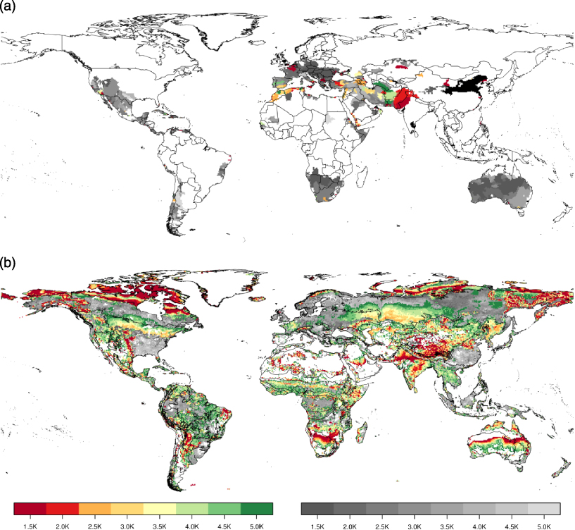
Figure 1. Threshold level of ΔTg leading to significant local changes in water resources (a) and terrestrial ecosystems (b). (a) Coloured areas: river basins with new water scarcity or aggravation of existing scarcity (cases (1) and (2), see section 2.3.1); greyish areas: basins experiencing lower water availability but remaining above scarcity levels (case (3)); black areas: basins remaining water-scarce but without significant aggravation of scarcity even at ΔTg = 5 °C (case (4)). No population change is assumed here (see figure S5 available at stacks.iop.org/ERL/8/034032/mmediafor maps including population scenarios). Basins with an average runoff <10 mm yr−1 per grid cell are masked out. (b) Regions with severe (coloured) or moderate (greyish) ecosystem transformation; delineation refers to the 90 biogeographic regions. All values denote changes found in >50% of the simulations.
Download figure:
Standard image High-resolution image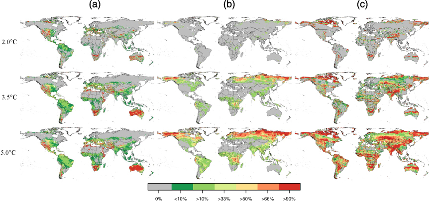
Figure 2. Likelihood of a decrease in runoff (a), an increase in runoff (b) and a severe change in ecosystems (c) for selected ΔTg levels. (a) and (b) show whether the simulated decrease (increase) in average annual runoff exceeds present (1980–2009) standard deviation, or whether monthly runoff is >10% more frequently below (above) its present median. Areas with presently <10 mm yr−1 are masked out. The likelihoods are derived from the 19 climate change patterns. See figures S1–S4 (available at stacks.iop.org/ERL/8/034032/mmedia) in the supplement for all eight ΔTg levels.
Download figure:
Standard image High-resolution imageTable 1. Continental and global effects of different ΔTg levels. Top: millions of people living in river basins characterized by chronic water scarcity (<1000 m3 cap−1 yr−1) (cases (2) and (4)), either with or without B1 and A2r future population change. People in water-scarce basins that show an aggravation of scarcity according to case (1) (see figure 3(a)) are not counted here. Numbers in brackets denote the changes (relative to the present) that are solely due to climate change. Bottom: number of unique biogeographic regions (out of 90) exposed to severe biogeochemical or vegetation structural shifts. All values refer to changes with >50% confidence, simulated under at least 10 of the 19 GCM patterns.
| Climate change only | Climate and B1 population change | Climate and A2r population change | |||||||||||
|---|---|---|---|---|---|---|---|---|---|---|---|---|---|
| Around 2000 | Affected | Total | Affected | Total | Affected | ||||||||
| Total | Affected | +2.0 ° C | +3.5 ° C | +5.0 ° C | +2.0 ° C | +3.5 ° C | +5.0 ° C | +2.0 ° C | +3.5 ° C | +5.0 ° C | |||
| People living in water-scarce basins | |||||||||||||
| Europe | 505 | 110 | 118 | 123 | 133 | 465 | 143 | 145 | 133 | 531 | 258 | 237 | 186 |
| Asia | 3879 | 870 | 988 | 985 | 970 | 3733 | 1424 | 1480 | 1442 | 6 929 | 3463 | 3440 | 3401 |
| Africa | 775 | 115 | 115 | 115 | 126 | 1647 | 313 | 304 | 295 | 3 145 | 1084 | 925 | 867 |
| N America | 479 | 83 | 81 | 86 | 87 | 712 | 137 | 121 | 127 | 891 | 270 | 274 | 259 |
| S America | 345 | 77 | 82 | 82 | 82 | 407 | 87 | 89 | 89 | 747 | 198 | 167 | 165 |
| Oceania | 29 | 13 | 13 | 13 | 14 | 44 | 16 | 18 | 18 | 55 | 19 | 20 | 20 |
| Globe | 6012 | 1267 | 1397 | 1404 | 1412 | 7009 | 2120 | 2157 | 2103 | 12 298 | 5294 | 5063 | 4897 |
| (+130) | (+137) | (+145) | (+628) | (+665) | (+611) | (+293) | (+62) | (−104) | |||||
| Number of unique biogeographic regions with severe ecosystem changes on >33% of their area | |||||||||||||
| Europe | 3 | — | — | — | 2 | ||||||||
| Asia | 22 | — | 1 | 6 | 16 | ||||||||
| Africa | 18 | — | 1 | 4 | 13 | ||||||||
| N America | 10 | — | 1 | 2 | 10 | ||||||||
| S America | 26 | — | 1 | 3 | 21 | ||||||||
| Oceania | 10 | — | — | 1 | 6 | ||||||||
| Globe | 90 | — | 4 | 16 | 68 | ||||||||

Figure 3. Continental-scale effects of selected ΔTg levels (2 ° C, left bars; 3.5 ° C, middle bars; 5 ° C, right bars), simulated under >50% of the climate change patterns. (a) Percentage of continental population exposed to new or aggravated water scarcity, or lower water availability outside water-scarce river basins, assuming unchanged population. (b) Percentage of continental endemism-weighted species richness of vascular plants in biogeographic regions exposed to substantial habitat shifts (Γ > 0.3 on >33% of the regions' area). The upper panel shows values relative to the continental totals, whereas the bottom panel shows values relative to the global totals. Numbers in brackets refer to the four cases of hydrologic change (see section 2 and figure 1). EUR, Europe; ASI, Asia; AFR, Africa; NAM, North America; SAM, South America; AUS, Australasia.
Download figure:
Standard image High-resolution imageConversely, more runoff is simulated especially for high latitudes and parts of the tropics at ΔTg > 3.5 °C (figure 2(b)). Associated shifts in seasonal hydrographs and higher flood risk compared to historical experience cannot be ruled out for those regions (Kundzewicz et al 2008), but this is not investigated in detail here as we focus on regions with decreases in runoff.
Many of the regions not significantly affected at ΔTg ≤ 2 °C are projected to become (more) water-scarce if Tg increased by up to 3.5 ° C—a scenario that cannot be dismissed, if no further commitments were made than current emissions reduction pledges. This concerns e.g. the Middle East, North Africa and South Europe (figure 1(a)), i.e. regions inhabited by another 3% of the world population (adding to the 8% increase at 2 ° C; see figure 4(a)). At ΔTg > 3.5 °C, the climate change effects expand further into these regions, such that 12–15% of each continent's population (Australasia, 23%) and 13% of the world population are exposed to aggravated or newly established water scarcity at ΔTg = 5 °C under >50% of the climate patterns (figure 3(a)). This increase is attributable primarily to Asia (see figure 3(a) bottom panel), while contributions from other continents are comparatively minor. Given the SRES B1 and A2r demographic projections, a higher fraction of the future world population would be exposed to water scarcity than around year 2000, i.e. 30–43% (∼2–5 billion cf table 1; also see figure S5 available at stacks.iop.org/ERL/8/034032/mmedia). Note that the relative increase in the number of people exposed to new or aggravated water scarcity due to climate change only is largely independent of the population scenario, as was also found by Gosling et al (2010).

Figure 4. Simulated exposure of world population to water scarcity (a) and of global endemism richness to severe habitat changes (b), plotted as functions of ΔTg. Left panel: function for all 8ΔTg levels and three confidence levels (stacked plot); right panel: results highlighted for 2, 3.5 and 5 ° C and the >50% case. Specifically, (a) shows the additional percentage of current world population exposed to new or aggravated water scarcity (cases (1) and (2); see section 2.3.1); (b) shows the percentage of global vascular plant endemism richness presently residing in regions that will be exposed to substantial habitat shifts (>33% of a region's area with Γ > 0.3). Grey bars in (b) show the corresponding number of affected regions (% out of the 90 regions; plotted on the same axis).
Download figure:
Standard image High-resolution image
3.2. Severe changes to terrestrial ecosystems
Substantial biogeochemical and vegetation structural shifts in terrestrial ecosystems are simulated under more than half of the climate patterns for a mean global warming of 2 ° C (figures 1(b) and 3). In particular, this concerns high latitudes (reflecting higher primary production and northward migration of the treeline), and also semiarid regions on all continents (reflecting CO2-induced improvements in plant water use efficiency and expanding vegetation cover) (Heyder et al 2011). These areas represent 11% of the ice-free, unmanaged global land surface (details in Ostberg et al 2013). But, due to the highly uneven distribution of species richness around the world, they represent only 4—albeit spatially quite extensive—unique biogeographic regions that altogether entail 1% of global endemism richness of vascular plants (table 1, figure 4(b)). The number of biogeographic regions exposed to severe habitat changes is found to quadruple at ΔTg = 3.5 °C, then affecting 10% of endemism richness. The incremental exposure steeply rises further if warming continued above this level: our simulations suggest that 68 out of the 90 distinct biogeographic regions—presently containing  of today's vascular plant endemism richness—would be subject to pronounced habitat transformation at 5 ° C (figure 4(b)). Even higher shares of continental endemism richness are reached in Africa and the Americas at 5 ° C (figure 3(b), top panel). Severe ecosystem changes on these two continents are simulated for regions presently containing half of the world's vascular plant endemism richness (see figure 3(b), bottom panel). Results tend to concur with regional studies that suggest significant declines in floral and faunal species richness at ΔTg above ∼3 ° C (Hare et al 2011).
3.3. Moderate or less confident changes
When choosing lower 'critical' thresholds (including non-water-scarce basins and, respectively, areas with 0.1 < Γ < 0.3) or considering changes simulated under less than 50% of the climate patterns, exposure to change generally occurs at lower ΔTg and covers larger areas. This is indicated by the following examples (figures compiled in the supplement available at stacks.iop.org/ERL/8/034032/mmedia). The incremental impact on ecosystems between 2 and 3.5 ° C is significantly stronger when accounting for moderate ecosystem changes in addition to severe ones, in terms of both the size of the affected area (figure S6(d) available at stacks.iop.org/ERL/8/034032/mmedia) and the number and endemism richness of the underlying biogeographic regions (figure S7 available at stacks.iop.org/ERL/8/034032/mmedia). If reductions in water availability are computed also for non-water-scarce basins in addition to the reductions in water-scarce regions, many regions especially in Europe, Australia and southern Africa appear to be affected already at 1.5 ° C (figure S6(a)). For a 5 ° C warming, this would mean that ∼20% of the world population is exposed to some form of significantly reduced water availability (figure S7). Finally, inclusion of unlikely changes (<33% of the simulations) suggests a substantially larger globally affected population (water scarcity) and area (ecosystem change) compared to the >50% case, for all ΔTg levels (figure S6). Note that 'unlikely' here represents changes that cannot be ruled out scientifically, as they occur under simulations from at least one of the 19 GCMs—each of which we here consider equally plausible.
4. Discussion
Albeit confined to selected change metrics, the present assessment accentuates asynchronies in exposure to climate change. That is, different regions are exposed to hydrologic or ecosystem changes at different ΔTg levels, as displayed in figure 1. Moreover, the study suggests that global and continental impacts accrue—in part nonlinearly—with ΔTg and that the shape of this growth curve differs between impact sectors.
For ecosystems, the climate response functions tend to display a sigmoidal shape with a slow initial increase, a rapid expansion in a critical range at intermediate ΔTg levels, and a plateau at high ΔTg when changes cover most regions (figure 4(b); note that the shape hardly depends on the confidence level, i.e. the number of climate scenarios). Regarding the additional population in water-scarce regions, the curve is much flatter, i.e. the incremental global effect of high ΔTg levels is weaker. It can also be noted, for Asia, that the population exposed to water scarcity slightly decreases at high ΔTg (table 1, representing case (2) category in figure 3(a) and possibly also basins that move out of the water-scarce category). This is probably due to nonlinearities in the relationship between forcing and hydrological response in a few, densely populated regions where e.g. effects of higher precipitation at high ΔTg may outdo effects of higher evapotranspiration. Detailed explanation of such developments would require model runs in which different driving forces are held constant. In general, different shapes of impact functions are found for change metrics other than those studied here, and also for individual regions (compare e.g. Levermann et al 2012, Schaphoff et al 2013).
Expert judgements suggest that abrupt, potentially irreversible biospheric 'tipping points' may be reached if ΔTg exceeds a critical range (Amazonian forest decline, +3–4 ° C; boreal forest decline, +3–5 ° C; Lenton et al 2008). While such events are not studied here, our results partly support these concerns. As shown in figure 1(b), widespread ecosystem changes and implied forest die-back in the southern boreal zone and some other regions are simulated under >50% of the climate patterns if ΔTg exceeded ∼3.5 ° C, due primarily to heat stress and also droughts (as is already evident in some regions; Allen et al 2010). However, large-scale change to Amazonian ecosystems—characterized by high endemism richness—is simulated only for ΔTg levels close to the maximum range considered here, i.e. 5 ° C (figure 2(c)). Recent findings also suggest that Amazonian die-back is found under a few climate change scenarios only, and that the (highly uncertain) CO2 effects on vegetation play a major role (Rammig et al 2010, Huntingford et al 2013). The simulated system transition in savannah-dominated regions agrees with recent evidence for local regime shifts (Higgins and Scheiter 2012), with C4 grass benefitting from low ΔTg and woody encroachment benefitting directly from the elevated CO2 concentration associated with higher ΔTg. Furthermore, in the boreal zone, permafrost thawing (not considered in the present model setup) will, due to higher microbial activity, augment soil carbon release even further than implied in our simulations, probably producing a positive feedback to warming (Schneider von Deimling et al 2012, Schaphoff et al 2013).
The here used climate change scenarios were constructed so that different ΔTg levels are reached around year 2100. In current high-emission scenarios, however, the prospective timing of ΔTg = 2 °C is around 2050 and that of ΔTg = 3.5 °C around 2080 (Rogelj et al 2012). Hence, in case such scenarios will come true, the demonstrated changes in water scarcity and Γ would occur some decades earlier than assumed herein. A related caveat, which merits quantification in further studies, is that the timing of ΔTg and associated local climate changes could be of importance. This is particularly true for ecosystems, whose adaptation capacities may be weaker or whose response to climate change may be slower than assumed in our model (Loarie et al 2009, Sandel et al 2011, Diffenbaugh and Field 2013). There is also scope to investigate how much of the difference in impacts between ΔTg levels is due only to the corresponding differences in atmospheric CO2 concentration. In fact, besides the radiative (climate) effects of CO2, there are direct physiological and structural effects on plants, with implications for both water scarcity and Γ. These effects are accounted for in the LPJmL model (Leipprand and Gerten 2006), but different assumptions about the relationship between CO2 and ΔTg (e.g. due to other emissions trajectories and climate sensitivities) may produce somewhat different responses. Furthermore, not only GCMs but also impact models (including vegetation models such as the one used here) differ in terms of model structure and parameterization, thus introducing a further level of uncertainty. Resulting uncertainties regarding the Γ metric and variants of the hydrologic metric used herein have been analysed recently (Piontek et al 2013, Schewe et al 2013).
5. Conclusions
Our comprehensive simulations show that both freshwater availability and ecosystem properties will change significantly in the future if no efforts were made to abate global warming. The impacts seem to accrue in nonlinear ways, though the shape of impact functions differs among the considered variables. Even if global warming was limited to 1.5–2 ° C above pre-industrial level in accordance with current negotiations, almost 500 million people might be affected by an aggravation of existing water scarcity or be newly exposed to water scarcity. Concurrent population growth would further increase this number to up to around 5 billion people. This outlook is basically supported by findings from Schewe et al (2013) based on a large suite of global hydrological models. Strongest effects on terrestrial ecosystems appear to occur at somewhat higher global warming levels, with the sharpest increase in the affected area (and underlying plant biodiversity) beyond 3–3.5 ° C. These global changes are simulated to be made up by a heterogeneous spatial pattern of change (which differs among impact variables), and different regions will be affected at different ΔTg levels (as summarized in figure 1).
Besides their obvious relevance for the affected regions themselves, the complex patterns of exposure to climate change might be of political and ethical concern when considering global mitigation targets and related impacts. For example, they shed interesting light on the ethical responsibility of high-emission countries, which—if accepted—could have bearing on both mitigation and adaptation burden sharing (Srinivasan et al 2008). Furthermore, the present results inform, but also complicate decisions about a fair allocation of international adaptation funds to different regions today. Such aspects will have to be explored in future studies, possibly relating the patterns of exposure to patterns of emissions underlying the climate change scenarios.
We emphasize that the here simulated changes to terrestrial ecosystems cover vast areas, which poses the question whether these changes are manageable, especially under conditions of rapid change and continued anthropogenic landscape modifications (Millar et al 2007). Decreases in water availability appear to be less widespread and may partly be buffered through adaptive management (not quantified here), even though climate change undermines the conventional assumption of stationary water resources (as reflected in our analysis of whether future changes exceed present variability; also see Milly et al 2008). At any rate, it is questionable whether adaptive water management will be sufficient to meet increasing water and food demands of a growing world population (Rost et al 2009). As a consequence, further expansion of irrigated or rainfed cropland may be needed, which would, in turn, amplify the climate change impact on Γ on those areas.
In sum, the present results plea for more comprehensive studies of whether critical ranges for a larger selection of impacts do cluster around a certain ΔTg level (as suggested already by Parry et al 2001, Schellnhuber et al 2004). Ultimately, this requires multi-sectoral impact model intercomparisons in an interdisciplinary scientific community effort, now under way (Arnell et al 2013, Piontek et al 2013).
Acknowledgments
This research was supported by the 6th and 7th Framework Programmes of the European Communities under grant agreements no. 036946 (WATCH) and 265170 (ERMITAGE), the BMBF-funded project GLUES, and the CGIAR research program on Climate Change, Agriculture and Food Security. We thank Katja Frieler and Malte Meinshausen for preparing the MAGICC6 data, Sibyll Schaphoff and Werner von Bloh for technical support, and anonymous reviewers for constructive comments.