
Abstract
Global agricultural models are becoming indispensable in the debate over climate change impacts and mitigation policies. Therefore, it is becoming increasingly important to validate these models and identify critical areas for improvement. In this letter, we illustrate both the opportunities and the challenges in undertaking such model validation, using the SIMPLE model of global agriculture. We look back at the long run historical period 1961–2006 and, using a few key historical drivers—population, incomes and total factor productivity—we find that SIMPLE is able to accurately reproduce historical changes in cropland use, crop price, crop production and average crop yields at the global scale. Equally important is our investigation into how the specific assumptions embedded in many agricultural models will likely influence these results. We find that those global models which are largely biophysical—thereby ignoring the price responsiveness of demand and supply—are likely to understate changes in crop production, while failing to capture the changes in cropland use and crop price. Likewise, global models which incorporate economic responses, but do so based on limited time series estimates of these responses, are likely to understate land use change and overstate price changes.
Export citation and abstract BibTeX RIS

Content from this work may be used under the terms of the Creative Commons Attribution 3.0 licence. Any further distribution of this work must maintain attribution to the author(s) and the title of the work, journal citation and DOI.
1. Introduction
Global agricultural models are indispensable in the debate over climate change impacts and mitigation policies. Recently these models have been used in analyses of land-based mitigation policies. This is important, since land-based emissions account for more than one-quarter of global GHG emissions [1], and could potentially supply 50% of economically efficient abatement at modest carbon prices, with most of this abatement coming from slowing the rate of agricultural land conversion [2]. Therefore, projections of agricultural land use are essential inputs to climate change and GHG mitigation studies. However, the value of such projections hinges on the scientific credibility of the underlying models. And this depends on model validation—an area in which global models of agriculture have been notably lacking to date.
Currently, there is great interest in redressing this limitation. However, the range of models currently in use is quite wide and the challenge of validation is a daunting one. Agricultural models can be loosely classified into two broad categories. On the one hand, there are 'partial equilibrium' models which specialize on the agricultural sector [3–5]. Often these models explicitly incorporate biophysical linkages between crop production and environmental variables. On the other hand, 'general equilibrium' models place agriculture within the context of the global economy, with most economic variables being endogenous to the model [2, 6, 7]. This makes validation more challenging and therefore most general equilibrium validation exercises focus on a few key variables or sectors [8, 9].
Successful model validation is also confounded by the fact that agricultural models must predict human behavior, as well as market interactions between economic agents. In particular, human decision making with respect to land use is context dependent, prone to change over time and poorly understood [10]. And even when these relationships are known, there is a lack of global, disaggregated, consistent, time series data for model estimation and evaluation of the full modeling system. In response to this challenge, some modelers have proposed a more targeted approach to validation by focusing on a few key historical developments or 'stylized facts' [11]. This suggests a useful way forward on validating agricultural models.
Without doubt, the most important fact about global agriculture over the past 50 years has been the tripling of crop production, with only 14% of this total coming at the extensive margin in the form of expansion of total arable lands [12]. This remarkable accomplishment contributed significantly to moderating land-based emissions [13]. Whether or not this historical performance can be replicated in the future is a central question in long run analyses of global agriculture [3, 6]. Yet studies which relate model projections to historical performance are quite sparse. For some models, evaluation of past agricultural projections has been mainly focused on crop production [14]. To our knowledge, only one global model currently in use has tackled the issue of reproducing historical cropland use [4].
We propose that long run global agricultural models of land use should be evaluated by looking back at the historical experience. In this letter, we illustrate the opportunity and the challenge of undertaking such an historical validation exercise using the SIMPLE model of global agriculture (Simplified International Model of agricultural Prices Land use and the Environment). As its name suggests, this framework is designed to be as simple as possible while capturing the major socioeconomic forces at work in determining global cropland use. This makes it a useful test-bed for the design of validation experiments. We test the model's performance against the historical period 1961–2006, illustrating what it does well and what it does poorly. Using this 45-year period as our laboratory, and focusing on the dimensions along which the model performs well, we then explore how various model restrictions which are embedded in many agricultural models alter SIMPLE's historical performance. These experiments serve to highlight which assumptions are likely to be most important from the point of view of cropland use. We then conclude with suggestions on how best to advance the state of our knowledge about modeling agricultural land use at the global scale.
2. SIMPLE: a global model of agriculture
Figure 1 outlines the structure of SIMPLE. A complete listing of equations and parameter values is provided in the supplementary online materials (SOM) (available at stacks.iop.org/ERL/8/034024/mmedia). The model's components can be divided between those contributing to the global demand for crops and those contributing to global crop supply. At the core of the supply-side are seven regional production functions generating crop output for the following continental scale regions: East Asia and Pacific, Europe and Central Asia, Latin America and Caribbean, Middle East and North Africa, North America, South Asia and Sub-Saharan Africa. These are calibrated to reproduce current yields in each region, as reflective of the existing technology, inherent land productivity, and non-land input use. Changes in any of these underlying factors will result in altered crop yields.
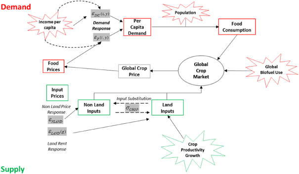
Figure 1. Overview of SIMPLE: the bottom panel (green) refers to supply regions for the aggregate crop commodity which are indexed by continent. The upper panel (red) refers to demand regions, indexed by income level. The disposition of crops includes direct consumption, feedstuff use and food processing, as well as biofuels. Adjustment of price in the global crop market ensures that long run supply equals long run demand.
Download figure:
Standard image High-resolution imageWe refer to the potential for increasing yields by applying more non-land inputs in response to land scarcity as the 'intensive margin of supply response' which is governed by the elasticity of substitution between land and non-land inputs: σCROP [15]. In contrast, the 'extensive margin of supply response' is governed by the elasticities of supply of land and non-land inputs to the crops sector: εLAND and εNLAND, which we set to their regional and long run values for this validation exercise [7, 8, 16]. Over the long run, changes in technology serve to shift the regional crop product supply schedules outward, so that more crop products will be delivered at a given market price and for a given input level.
The global demand for crop output is comprised of feedstocks for biofuels (exogenous in our model) as well as direct food consumption by households, feedstuffs for livestock and crop inputs to processed food production. Livestock and processed foods are value-added products and are conceptualized in this model as being produced and consumed within each demand region using crop and non-crop inputs. In our baseline, income levels differ across the five consuming regions, based on their categorization by the World Bank [17] in the year 2001: low income countries (including India), lower middle income countries (including China), upper middle income nations (including Brazil), lower high, and upper high income countries. A large share of crop demands in SIMPLE are derived demands, originating from the consumer demands for livestock and processed food products. This is important, since technological change and factor substitution in these sectors can alter the intensity of crop use in producing these food products. It is assumed that only the livestock sector has the ability to conserve on crop inputs (via input substitution or reduction of waste) in response to higher prices and this is captured by the elasticities of substitution between feed and non-feed inputs: σLSTK.
The demand for food in the income regions is a function of population, per capita income and commodity prices. The latter are governed by the income and price elasticities of demand, εY(i,y) and εP(i,y), which vary by commodity type (crop, livestock, processed foods) as well as consumers' income level [18]. In particular, food demands in regions with high per capita incomes are less responsive to changes in both income and prices, whereas low income consumers have little choice but to reduce consumption when food prices rise, since food makes up a relatively large share of their household's budget, and they tend to respond to higher incomes by consuming more food and upgrading their diets.
Long run equilibrium in SIMPLE is attained when global crop supply equals global demand where the equilibrating variable is the global crop price. Note that SIMPLE is a static partial equilibrium model of global agriculture so projections are calculated from one point in time (e.g., 1961) to another (e.g., 2006). The model does not attempt to predict the path by which land changes between those points.
3. Model validation
Given our interest in projections of global land use change to 2050, we choose to evaluate the SIMPLE model over a comparable period of time—in this case from 1961 to 2006.1 The most obvious metrics involve comparing endogenous predictions to observed changes in the following global scale variables: (a) crop production, (b) crop price, (c) cropland area, and (d) average crop yield. To derive these endogenous changes in SIMPLE, we perturb the model using the main exogenous drivers of global agriculture during this historical period, including: population and per capita income (by demand region) and total factor productivity (TFP) for crops (by supply region), livestock and food processing (by demand region). The values for these exogenous drivers, which were derived from several studies [19–23], are reported in table 1. Looking at the table, we see that population and per capita incomes grew steadily during this historical period. Notable growth in population can be observed in the lower high, upper middle (such as Brazil) and low income regions (such as India). Likewise, we observe steady growth in per capita incomes with the lower middle income region (including China) showing sharply higher per capita income growth (4.3% per annum). Crop supplies are mainly driven by the growth in TFP which is the key measure of productivity improvement in the model. For the crop sector, TFP grew by more than 1.2% per annum, with the exception of Sub-Saharan Africa where it grew by 0.9% annually. With regard to the livestock sector, we observe strong TFP growth in the lower middle income region. In contrast, livestock TFP growth in the low income region grew by only 0.2% per annum. Due to lack of reliable regional estimates, we impose a uniform rate in the TFP growth in the processed food sector across all regions.
Table 1. Per annum growth rates of exogenous drivers for the historical period 1961–2006.
| Income regions | Population | Per capita income | Total factor productivity | Geographic regions | ||
|---|---|---|---|---|---|---|
| Livestock | Processed food | Crops | ||||
| Upper high | 0.79 | 2.62 | 0.92 | 0.74 | 1.89 | East Asia and Pacific |
| 1.78 | Europe and Central Asia | |||||
| Lower high | 2.64 | 2.69 | 0.92 | 1.58 | Latin America and the Caribbean | |
| Upper middle | 2.07 | 1.71 | 0.75 | 2.19 | Middle East and North Africa | |
| Lower middle | 1.71 | 4.25 | 2.20 | 1.65 | North America | |
| 1.15 | South Asia | |||||
| Low | 2.26 | 2.35 | 0.16 | 0.91 | Sub-Saharan Africa | |
| Sources | UN World Population Prospects [19] | Ludena et al [21] | Emvalomatis et al [22] | Fuglie [23] | ||
| World Development Indicators [20] | ||||||
As with any global model, some tuning is necessary in order to ensure reasonable performance of the integrated, equilibrium model. However, we refrain from tuning the model over the full period for which the historical validation is undertaken (i.e. 1961–2006), focusing instead on the period 2001–2006. The model keys on three dimensions of global agriculture, namely the economic response of crop yields to crop prices, intensification parameters for the livestock and processed food sectors and the demand response for food commodities. Details of the tuning process are included in the SOM.
Global validation results are reported in figure 2 (see SOM table 4 for details available at stacks.iop.org/ERL/8/034024/mmedia). From the figure, we see that SIMPLE slightly overstates the global change in crop production over the 1961–2006 period (206% versus 196%). The model also slightly understates the historical decline in crop price (24% versus 29%). SIMPLE does a very good job in predicting the partitioning of supply growth between the intensive and extensive margins, with changes in global cropland and global average crop yield (17% and 162%, respectively) slightly above the observed values (16% and 156%, respectively) due to the higher level of global output. Overall, we are pleased with these global results and are more confident that SIMPLE incorporates the key drivers and economic responses that govern long run changes in agriculture, at the global scale. We will draw on these global results again in section 4 to explore the implications for assumptions embedded in agricultural models currently in use.
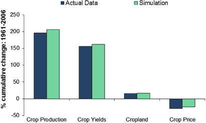
Figure 2. Global results of the historical validation experiment (1961–2006). The bars show the per cent changes in (from left to right) global crop production, yield, land use and price computed from actual data (dark blue bar) and from the simulation results (light green bar). The historical experiment is conducted using the SIMPLE model given exogenous historical growth in population, per capita income and total factor productivity growth in agriculture after calibrating the model over the 2001–2006 period.
Download figure:
Standard image High-resolution imageBefore we proceed further, however, it is important to note that the regional results on cropland and production are much less satisfactory than the global results (figure 3, SOM table 4), with too little area expansion in East Asia and Pacific, Latin America and Caribbean and Sub-Saharan Africa, and too much expansion in other regions. Indeed, SIMPLE is unable to capture the reduction in cropland area in North America and Europe. However, our results are consistent with the literature. Other agricultural models also find it difficult to capture changes at the regional levels [14]. As we move from global to regional projections, regional drivers become more important. In the case of SIMPLE, we attribute the discrepancies in the regional results to the absence of domestic agricultural and foreign trade policies, as well as the fact that we abstract from other barriers to trade, including poor infrastructure and administrative obstacles.
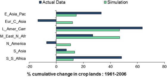
Figure 3. Regional changes in cropland use from the historical validation experiment (1961–2006). The bars show the per cent changes from actual data (dark blue bar) and from the simulation results (light green bar).
Download figure:
Standard image High-resolution imageFundamental to SIMPLE's allocation of global production across regions is the assumption of fully integrated global crop markets. Yet this was far from the truth throughout most of our historical period. This state of affairs was highlighted by Johnson who published a series of papers and books on the topic of 'World Agriculture in Disarray' [24] over the post WWII period. In this work, Johnson discusses the many distortions which caused the global distribution of agricultural output to be inconsistent with economic logic. The evolution of these distortions has subsequently been documented in a path-breaking study by Anderson [25]. Since the completion of the Uruguay Round of talks, which resulted in establishment of the World Trade Organization, agricultural support has been reformed in many parts of the world. However, there remain significant barriers to free trade in agricultural products [26] and this suggests the need to incorporate such policies into SIMPLE if it is to accurately reflect the regional evolution of future production.
In addition to explicit government policies shaping the regional patterns of agricultural production, there are other important barriers to international trade in agricultural products, including poor quality domestic transport infrastructure, burdensome customs procedures and poorly developed port facilities. These barriers to trade loom particularly large in Sub-Saharan Africa [27], and have limited that regions' engagement in the global trading system. As a consequence of this insulation from world markets, Sub-Saharan Africa's output has grown much more than would have been anticipated, given its relatively low rate of productivity growth over the 1961–2006 period. And its increased output has largely been directed to domestic consumption. This is reflected in the fact that its share in global trade of agricultural products has declined by around 70% during this historical period [28].
In summary, our validation experiment suggests that, while SIMPLE is adept at capturing long run changes in output and land use at global scale, the problem of allocating these changes across regions is far more challenging. In light of these findings, we will restrict our analysis in section 4 to global scale variables.
4. Evaluating key assumptions in other global models
Existing global agricultural models produce significantly different projections of global land use in 2050 [29]. This is hardly surprising, given the widely varying assumptions embedded in the models. Some of these differences may be inconsequential for simulating global land use change, while others may be critically important. Absent a laboratory in which to test these alternative assumptions it is impossible to know which model results are reliable. For this reason, we believe that it would be invaluable to have a standard set of validation experiments against which to evaluate model performance, test new features, and set future research priorities.
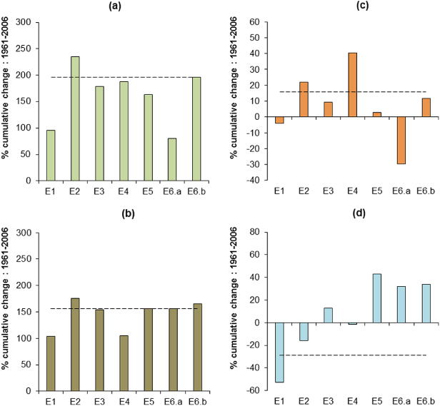
In this section, we introduce such a set of experiments, each focusing on a specific restriction to the SIMPLE model, aimed at highlighting the consequences of each assumption for global land use change. These restrictions have been chosen to highlight shortcomings in existing global models, allowing us to assess their relative significance. They include: exogenous per capita food consumption (E1), fixed price and income elasticities of demand for food (E2), short- to medium run input supply elasticities (E3), the absence of endogenous intensification of crop production (E4) and historical trend-based yield projections (E5). To illustrate the potential for interactions amongst these restrictions, we also consider two experiments (E6.a and E6.b) which include multiple elements of the earlier experiments designed to reflect combinations of assumptions sometimes found in biophysical and in economic models of global agricultural land use.
Figure 4 summarizes the results from these restricted experiments. In every case, the key historical drivers of change—population, income and total factor productivity growth—are identical to our historical baseline. We first look at restrictions in the way crop demand is modeled and start with the simplest possible assumption, namely exogenizing per capita food consumption as is done in some versions of agricultural models with limited consumer demand systems [6]. As illustrated in figure 4, preserving the historical per capita food consumption (E1) leads to an understatement of the increase in global crop demand and global crop production over this historical period. With less output growth, but the same level of TFP growth, prices fall sharply, yields grow more slowly, and global cropland use contracts.
Figure 4. Global results of the evaluation experiments (1961–2006). The panels show the per cent changes in crop production (a), yield (b), land use (c) and price (d) computed from actual data (dashed line) and from the simulation results (colored bars). The experiments consists of (E1) exogenous per capita consumption, (E2) fixed food demand response, (E3) short to medium run supply response, (E4) restricted intensive margin, (E5) targeted crop yields, (E6.a) combined exogenous per capita consumption, restricted intensive margin and targeted crop yields, and (E6.b) combined fixed food demand response and short to medium run supply response.
Download figure:
Standard image High-resolution image
A more common consumption specification in global agricultural models is to have fixed (unchanging) price and income elasticities of food demand [3, 5]. In this case, rather than becoming smaller in absolute value as per capita incomes rise (recall figure 1) [18], the responsiveness of demand to rising incomes is based on historical estimates of these values and is kept constant (E2). In this case, we observe in figure 4 that both global crop demand and global crop production are overstated. This is due to the dominance of the income effect over this projections period. With sharply rising incomes, a failure to account for the diminishing impact of marginal increments to purchasing power results in excessively high demand and a significant overstatement of historical production, area and yield, while global crop price falls by only about half of its observed value.
Let us now turn from the demand to the supply-side of the global agricultural picture—recall that there are two key margins of economic response here: the extensive margin (additional area) and the intensive margin (yield increases). We begin with the parameters which influence the extensive margin. Specifically, in E3 we replace the long run supply elasticities for land and non-land inputs with their corresponding short run (five year) values as were used in our 2001–2006 tuning exercise [7]. Models which are based on econometric estimates of cropland area response are likely to fall prey to this limitation [2, 5]. This is because most such estimates are based on annual time series data from which it is hard to extract long term supply response. This point is emphasized by Hertel [30] who offers indirect evidence that prominent global studies of biofuels [31] and climate impacts [5] are likely not using long run elasticities in their models. With these short run parameters in place, the results in E3 show how a smaller global supply response leads to a rise in crop prices over this period, as cropland area is unable to respond as vigorously to increased land demand for crop production. While yield changes are comparable to their historical values over this period, production falls short of its historical value, despite the rising crop prices.
The other critical component of supply is the response of yields to higher crop prices and/or increased scarcity of land. While the size of this response is hotly debated [15, 32–34], there is little doubt that significantly higher prices do encourage farmers to respond with more intensive cultivation practices. Yet not all agricultural models incorporate this possibility [35], and it is often unclear how large this effect is in those models that do allow for endogenous yield response [3–5]. We explore this issue in experiment E4 which eliminates this intensive margin of supply response. As a consequence, yields grow more slowly than in the historical record—being driven solely by TFP growth. Crop prices are essentially flat and cropland expansion is in excess of 40%—as opposed to the observe change of just 16%. Clearly failure to account for the intensive margin of supply response can be expected to lead to a significant overstatement of future cropland requirements.
A slightly different approach involves explicitly targeting the rate of average crop yield growth (as opposed to targeting TFP). This is relevant, since many biophysically based agricultural models treat productivity growth as arising largely through crop yield improvements [3–5]. Of course, if we knew in the future how fast yields were to grow, one can expect that we would be far closer to our goal of making credible projections of global land use change. But, as experiment E5 demonstrates, even knowing yields with certainty does not allow us to predict cropland change accurately over this historical period. Since land is only one of many agricultural inputs, accurately projecting yields does not allow for an accurate prediction of the change in crop prices over time, as can be seen from the bar for E5 in the lower right panel in figure 4. This in turn leads to the underestimation of the changes in crop production and cropland use.
The last two experiments illustrate the potential impacts in our historical projections when we combine some of the above restrictions. We start with a biophysical view of the historical period wherein per capita food consumption is exogenous, the crop yield response to higher crop prices is absent (i.e. no intensive margin) and crop yield growth is targeted (E6.a). Similar to our first experiment, we observe that global crop production is grossly understated (upper left panel of figure 4). By targeting average yields and ignoring the economic yield response, we see that the changes in global cropland use and global crop price move in the opposite direction of what was observed over this historical period.
Another interesting combination of restrictions is captured by E6.b, which seeks to mimic the behavior of those global agricultural models which fail to account for long run changes on the demand and supply sides. Specifically, we do not allow the price and income elasticities of demand for food to evolve with per capita incomes, and we use the short to medium run input supply elasticities. With an overly responsive demand for food, our projections tend to capture the rise in global crop production but erroneously predict the change in global crop price. As the supply of land is less responsive to land rents, global crop demand can only be met by increasing the use of non-land inputs; hence, global average crop yields are overstated while global cropland expansion is understated under this scenario.
5. Summary and conclusions
In this study, we illustrate an approach to validating agricultural land use in global models by looking back at the historical experience from 1961 to 2006. Using the SIMPLE model, we successfully replicate historical changes in global crop production, cropland use, average crop yield and crop price using only population, incomes and total factor productivity as the key drivers of agriculture. However, the model performs relatively poorly in the geographic distribution of production and land use changes over this period which suggest that there are regional drivers and market barriers which are not captured in SIMPLE. Addressing these limitations will require further research and refinement of the framework. In the meantime, we believe there is still great value in testing existing agricultural models at global scale, comparing predicted changes in production, land use and crop prices to observed values.
Using our framework we were able to highlight critical assumptions within existing agricultural models that are likely to have a significant impact on global outcomes. Scientists who use such models for long run projections should be aware of the implications of these assumptions. We find that those models which are largely biophysical—and ignore the price responsiveness of demand and supply—likely understate changes in crop production, while failing to capture the changes in cropland use and crop price. On the other hand, those models which incorporate economic responses based on statistical estimation of key parameters using limited time series estimates likely understate long run supply and demand responses to crop price. We find that when these shorter run assumptions are imposed on SIMPLE over the 45-year test period, the model tends to over-predict historical output changes, while understating land use change. By testing each global agricultural model against the historical record, researchers can better understand where their models succeed or fall short. This will aid in prioritizing areas for model improvement.
Acknowledgments
The authors thank Petr Havlik, David Lobell, Hermann Lotze-Campen, Tony Janetos and Peter Verburg for valuable comments on an earlier version of this letter. They acknowledge support for the underlying research into the climate–food–energy–land–water nexus from US Department of Energy, Office of Science, Office of Biological and Environmental Research, Integrated Assessment Research Program, Grant No. DE-SC005171.
Footnotes
- 1
One issue which must be confronted in such a validation exercise is whether to report the results going backwards in time, or going forward. In principle, we prefer the backwards approach (i.e. going from 2006 back to 1961). However, in practice we found this very confusing. Therefore, we first simulate the model backwards to 1961, thereupon establishing an historical equilibrium. We then undertake the validation experiment by simulating the model forward again to 2006, comparing these results to the observed changes over this period.